Quantitative Similarity-Based Association Tests Using Population Samples

Abstract

Although genetic association studies using unrelated individuals may be subject to bias caused by population stratification, alternative methods that are robust to population stratification, such as family-based association designs, may be less powerful. Furthermore, it is often more feasible and less expensive to collect unrelated individuals. Recently, several statistical methods have been proposed for case-control association tests in a structured population; these methods may be robust to population stratification. In the present study, we propose a quantitative similarity-based association test (QSAT) to identify association between a candidate marker and a quantitative trait of interest, through use of unrelated individuals. For the QSAT, we first determine whether two individuals are from the same subpopulation or from different subpopulations, using genotype data at a set of independent markers. We then perform an association test between the candidate marker and the quantitative trait, through incorporation of such information. Simulation results based on either coalescent models or empirical population genetics data show that the QSAT has a correct type I error rate in the presence of population stratification and that the power of the QSAT is higher than that of family-based association designs.

Introduction

Population-based association studies using unrelated individuals have often been criticized for inducing spurious associations due to population stratification. As a result, family-based association designs (Spielman et al. 1993) have received great attention recently, because of their robustness to population stratification and their potentially higher power relative to linkage studies (Risch and Merikangas 1996). Population samples consisting of unrelated individuals, however, may be easier and less expensive to collect, and such designs are, in general, more powerful than family-based association designs, both for qualitative traits (Morton and Collins 1998; Risch and Teng 1998; Teng and Risch 1999; Risch 2000) and for quantitative traits (van den Oord 1999). Recently, several methods have been proposed that utilize genomic markers to control for population stratification in the analysis of unrelated individuals (Devlin and Roeder 1999; Bacanu et al. 2000; Pritchard et al. 2000b; Reich and Goldstein 2001; Satten et al. 2001; Zhang et al., in press). These novel approaches are promising because they may have greater power than family-based association designs and may be robust to potential population stratification. One limitation of these methods is that they are only applicable to qualitative traits, although quantitative traits may contain more information.

In the present study, we develop a quantitative similarity-based association test (QSAT) to examine associations between candidate markers and quantitative traits of interest, in a set of unrelated individuals. The QSAT controls population stratification through a set of genomic markers. To perform the QSAT, we first use the genotypes of the sampled individuals at a series of independent markers to calculate a similarity score, S_ij, between individuals i and j. We then model the distribution of these similarities, through use of a normal mixture model with one or two components (a within-subpopulation component and a between-subpopulation component). We then use the Bayesian information criterion to estimate the number of components and decompose each individual’s genotypic score into within-subpopulation and between-subpopulation components. The QSAT is then calculated on the basis of a regression model that treats the trait value as the dependent variable and the within- and between-population genotypic scores as predictors. We evaluate the performance of the QSAT through simulations using coalescent models and empirical population genetics data. The simulation results suggest that our procedure has a correct type I error rate in the presence of population stratification and is more powerful than statistical association tests for family-based association designs (Fulker et al. 1999; Monks and Kaplan 2000; Sun et al. 2000).

Methods

In this section, we first discuss the method for a homogeneous population and then discuss the QSAT for a heterogeneous population. We assume that the candidate marker is biallelic, with alleles M and m. There are three genotypes at this marker: MM, Mm, and mm. For an individual, we use A to denote the additive genotypic score at the candidate marker, with the value of A being 1, 0, and −1 for genotypes MM, Mm, and mm, respectively. We use D to denote the dominance genotypic score at the candidate marker, with the value of D being 0, 1, and 0 for genotypes MM, Mm, and mm, respectively. Let y_i denote the quantitative trait value of the ith individual. For a homogeneous population, genetic association between the candidate marker and the quantitative trait can be studied through the following regression model:

where the values of e_i are assumed to be independent of each other and independent of the values of A_i and D_i, with mean 0 and variance σ². In this regression model, α and β are the additive and dominance genetic values. In the case of a homogeneous population, the least-squares (LS) estimators of α and β, denoted by and , respectively, are unbiased estimators of α and β. Under the null hypothesis of no association between the candidate marker and the trait of interest, both α and β are 0, and standard statistical tests can be performed to identify deviation from the null hypothesis.

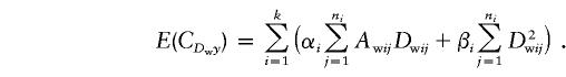
The regression method shown in equation (1) may be invalid in the presence of population stratification. To illustrate this point, let us assume that there are k subpopulations, with n_i individuals sampled from the ith subpopulation, and that each subpopulation is homogeneous. Let μ_i denote the phenotype mean in the ith subpopulation, let p_i and q_i denote the allele frequencies of the M and m alleles in the ith population, let y_ij denote the trait value of the jth individual in the ith subpopulation, and let A_ij and D_ij denote the additive and dominance genotypic scores of the jth individual in the ith subpopulation. We assume that the conditional expectation of the trait value of the jth individual in the ith subpopulation is

In the presence of subpopulations, the null hypothesis to be tested is that there is no association between the candidate marker and the trait value in any of the subpopulations—that is, α₁=…=α_k=0 and β₁=…=β_k=0.

If we apply the following regression model to test the null hypothesis of no association between the candidate marker and the trait,

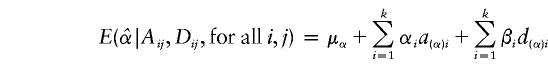
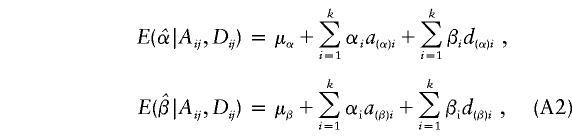
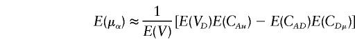
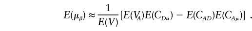
the conditional expectations of regression coefficients and , conditional on the observed values of A_ij and D_ij, are

and

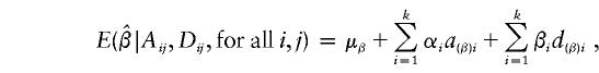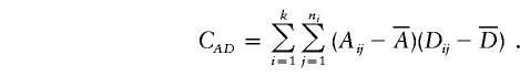
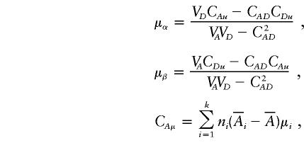
where the notation is given in detail in Appendix A, with , and . Under the null hypothesis of no association between the candidate marker and the trait of interest, α₁=…=α_k=0 and β₁=…=β_k=0, , and . Therefore, and , under the null hypothesis; however, E(μ_α) and E(μ_β) may not be 0, in general, when allele frequencies and mean trait values differ among the subpopulations. Therefore, in the presence of population stratification, even under the null hypothesis of no association between the candidate marker and the trait of interest, statistical tests based on the model in equation (3) may lead to false positives due to population stratification.

In the context of analyzing sib-pair data, Fulker et al. (1999) proposed to decompose the genotypic score into two orthogonal components: the between-family (b) component and the within-family (w) component. Under this decomposition, only the between-family component is sensitive to population structure, and the within-family component is significant only when there is an association between the candidate marker and the trait. This approach has been extended to nuclear families (Abecasis et al. 2000) and general sibship data (Sham et al. 2000). To generalize this idea to population data in cases in which the exact population structure is known, we can decompose the genotypic scores into orthogonal between-population and within-population components. Specifically, we define and to be between-population and within-population additive genotypic scores, respectively, and define and to be between-population and within-population dominance genotypic scores, respectively. Having defined the notation, we consider the following regression model:

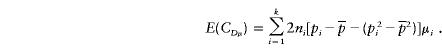
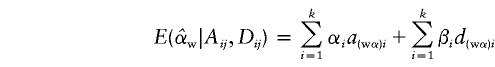
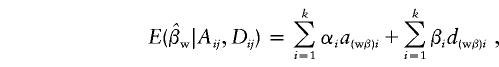
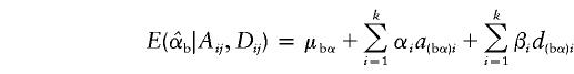
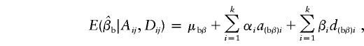
Denote the LS estimators of α_b, α_w, β_b, and β_w as , , , and , respectively. The conditional expectations of these estimators are derived in Appendix B, and it can be shown that all the spurious association between genotypic scores and trait values due to population stratification is accounted for by and . On the other hand, and are unbiased estimates of the additive and dominance genetic values α* and β*, provided that all subpopulations have the same additive and dominance genetic values—that is, α₁=…=α_k=α^* and β₁=…=β_k=β^*. When the additive and dominance values are different among the subpopulations, the expectations of and are

and

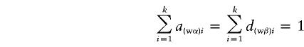
where and , and the details are given in Appendix B. So, under the null hypothesis of no association, and . Intuitively, when all of the subpopulations have the same additive and dominance genetic values (the mean trait values may be different among subpopulations), then α₁=…=α_k=α_w and β₁=…=β_k=β_w. In this case, testing the hypothesis H₀:α₁=…=α_k=0 and β₁=…=β_k=0 is equivalent to testing the hypothesis H¹₀:α_w=β_w=0 under the model in equation (4). When the additive and dominance genetic values vary among subpopulations, α_w and β_w are linear combinations of α_i and β_i. In this case, rejection of H¹₀ guarantees rejection of H₀. Therefore, the test for the null hypothesis H¹₀ under the model in equation (4) is still a valid test for hypothesis H₀ in a structured population.

One difficulty in the application of the above approach is that we do not know the underlying population structure. However, potential population structures can be estimated through a series of genetic markers (e.g., see the report by Pritchard et al. [2000a]). In the present study, instead of estimating the underlying population structure, we examine each pair of individuals and infer whether the two individuals are from the same subpopulation or from different subpopulations. Suppose that there are L independent biallelic markers 𝒜_l, where l=1,…,L, and each marker 𝒜_l has two alleles, A_l and a_l. Further suppose that there are n individuals in our sample and let z_il denote the genotype of the ith individual at the lth marker, where i=1,…,n and l=1,…,L. The value of each z_il can be 0, 1, or 2, corresponding to the ith individual having 0, 1, or 2 copies of allele A_l, respectively. A natural measure of the difference in genotypes between the ith and the jth individuals is . In the present study, we define the similarity, S_ij, between the ith and the jth individuals as S_ij=d_max-d_ij, where d_max is the maximum value of the d_ij across all pairs of individuals.

For individuals within the same subpopulation, we expect the value of S_ij to be smaller than that between individuals from different subpopulations. We propose to decompose these similarity estimates into two components: a within-subpopulation component and a between-subpopulation component. To identify possible components among the S_ij, we assume the following normal mixture model for the similarity estimates S_ij:

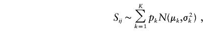where K represents the number of components in the mixture model, p_k denotes the proportion of the kth component, and N(μ_k,σ²_k) denotes the Gaussian density function with mean μ_k and variance σ²_k. The maximum-likelihood estimates of the parameters p_k, μ_k, and σ_k, for a given K, can be obtained by means of the clustering expectation-maximization (CEM) method (Celeux and Govaert 1995). We use the Bayesian information criterion (BIC) to choose K. The BIC is defined as BIC(K)=-2L(K)+M(K)logN, where N is the total number of observations,

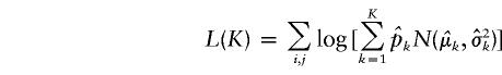is the maximized log likelihood for a given K, and M(K) is the number of free parameters in the mixture model. On the basis of our experience with simulated data sets based on both coalescent models and on empirical population genetics data, a choice for K between 1 and 2 is adequate to account for population structure in the data. The case of K=1 corresponds to a single population—that is, there is no population heterogeneity, whereas K=2 corresponds to two components: a within-population component and a between-population component. Note that K=2 implies only that there is population structure in the data, but it does not imply that there are only two subpopulations. When K=2, let , , and denote the maximum-likelihood estimates of the parameters p_k, μ_k, and σ_k, respectively; then

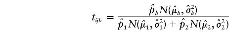is the conditional probability that S_ij arises from the kth mixture component. Assuming that if t_ij1>.5, we define the similarity indicator W_ij between the ith and the jth individuals to be 1 and assume that these two individuals belong to the same subpopulation in our subsequent analysis. If t_ij1<.5, we define the similarity indicator W_ij between the ith and the jth individuals to be 0 and assume that these two individuals belong to different subpopulations.

Let y_i, A_i, and D_i denote the trait value, additive genotypic score, and dominance genotypic score, respectively, of the ith individual. Let , with n_i defined as the number of individuals estimated to be in the same subpopulation as the ith individual. Using A_i and W_ij, we can decompose the additive genotypic score, A_i, into two components: a between-subpopulation component, , and a within- subpopulation component, . Similarly, we can decompose the dominance genotypic score, D_i, into two components: a between-subpopulation component and a within-subpopulation component . On the basis of these definitions, we fit the following regression model:

When there are k subpopulations, and under the assumption that we can make correct inference about whether two individuals are from the same or different subpopulations, the between-subpopulation components and the within-subpopulation components are orthogonal. The LS estimates of α_w and β_w are

and

where

and

To test the null hypothesis that there is no association between the candidate marker and the trait of interest in all subpopulations, we may test the null hypothesis H₀:α_w=β_w=0, through use of the regression model in equation (5). If we assume that e_i are independent normal variables with the same variance, the usual test statistic is the F test statistic, , where , ,

and is an estimate of the variance of the e_i. However, the e_i may not follow the normal distribution and may not have the same variance, especially for different genotypes and in different subpopulations. Therefore, statistical inferences using the F statistic may not lead to correct statistical significance levels.

In the present study, we propose to use T as our QSAT and to use simulations to evaluate statistical significance for the test statistic. The basic idea of the simulation method is to permute the trait values of the individuals within the same subpopulation, in order to derive an empirical distribution for the test statistic; however, one practical difficulty in implementing this method directly is that we do not know exactly how many subpopulations there are or which individuals belong to the same subpopulation. As a result, we propose the following simulation method to approximate the distribution of the QSAT:

• 1. Randomly choose one individual—say, the i₁th individual—in the sample. Then randomly choose one individual from the set {i:W_i1i=1}—say, the i^*₁th individual. Denote the trait value of the i^*₁th individual as y^*_i1;
• 2. Randomly choose one individual from all sampled individuals except the i₁th individual—say, the i₂th individual. Then randomly choose one individual from the set I_i2={i:W_i2i=1}/{i^*₁}—say, the i^*₂th individual. Denote the trait value of the i^*₂th individual by y^*_i2. If I_i2 is an empty set, define y^*_i2=y_i2;
• 3. Randomly choose one from all the sampled individuals except individuals i₁,i₂,…,i_(j-1)—say, individual i_j—and randomly choose one individual from the set I_ij={i:W_iji=1}/—individual i^*_j, for example. Denote the trait value of i^*_jth individual as y^*_ij. If I_ij is an empty set, define y^*_ij=y_ij.

In the end, we generate a set of new trait values: y^*₁,y^*₂…, and y^*_n for the n individuals in the sample. For this simulated sample, we calculate the test statistic. We repeatedly generate m sets of simulated data sets, and we can then estimate the level of statistical significance from these test statistics.

Simulation Models

In this section, we discuss the simulation models used to assess whether the QSAT is robust to population stratification and to compare the power of the QSAT with other association tests. In our simulation studies, we generate the data either through coalescent models or through empirical population genetics data.

Coalescent Models

In this set of simulations, we use coalescent models to generate genotypes of the sampled individuals in a structured population. Pritchard et al. (2000b) considered coalescent models with constant population sizes. We consider coalescent models with variable population sizes (Griffiths and Tavaré 1994, 1997) in our simulations and allow subpopulations to have different population sizes. We assume that there was an ancestral population that had evolved for a long period of time with a constant population size; this population was then divided into two subpopulations, T generations before the present time. From the time of division, the two subpopulations have experienced exponential growth independently, without migrations. We assume that, at the time of division, the population sizes of the two subpopulations were 100 and 10⁴, respectively, and that the population sizes at the present time are 10⁷ and 5×10⁷, respectively. Therefore, the first subpopulation has experienced more rapid growth than has the second subpopulation. We consider three population divergence times between the two subpopulations: (1) T=500 generations, (2) T=1,500 generations, and (3) T=4,500 generations. The first two separation times probably correspond to the divergence time between non-African populations, and the third separation time probably corresponds to the divergence time between African and non-African populations (Goldstein et al. 1995).

We assume that a total of 500 independent biallelic markers are used for our inference on the population structure. The sample consists of 25 individuals from the first subpopulation and 125 individuals from the second subpopulation. We assume that the mutation rate is μ=5×10^-7 per generation and only select markers with allele frequencies of ⩾.2 in the sample. This threshold was also used by Pritchard and Rosenberg (1999) to approximate the likely characteristics of single-nucleotide polymorphism (SNP) surveys (Wang et al. 1998). We use the same procedure to simulate genotypes at the candidate locus. On the basis of the genotype at the candidate locus, the trait values are generated according to the following model:

where μ_i=μ₀₀×R_i, α_i=β_i=μ₀×R_i, and e_ij is a normal random variable or a log-normal variable with mean 0 and variance 1. In our simulations, we set R₁=1 for individuals from the first subpopulation, R₂=1/4 for individuals from the second subpopulation, and μ₀₀=2. Furthermore, we set μ₀=0 and μ₀=2, for the type I error examination and power comparison, respectively. We also vary genetic models and trait distributions (either normally distributed or log-normally distributed) in our simulations. In the determination of the allele that increases the quantitative trait values, we fix the same allele in the two subpopulations.

Empirical Population Genetics Data

One limitation of the simulations based on coalescent models is that these models may not represent the human population evolutionary histories accurately. Therefore, in our simulations, we also use empirical population genetics data from the population genetics database ALFRED (Osier et al. 2001; ALFRED Web site), which provides allele frequencies for SNPs and for microsatellite markers in different populations. For our simulations, we extracted 130 markers across four populations, including Danes, San Francisco Chinese, Biaka, and Maya. We use these four populations to represent populations from four different continents. For microsatellite markers, we pool the alleles to form biallelic markers with allele frequencies of 10%–90%.

For simulations based on empirical population genetics data, we consider different numbers of markers used to infer pairwise relationships, different trait-value distributions, and different schemes to assign alleles conferring high trait values. We generate 20 replications, with each replication consisting of a total of n individuals. Among these n individuals, there are .5n individuals sampled from the Danes, .2n individuals from the Chinese, .2n individuals from the Biaka, and .1n individuals from the Maya. In the determination of the allele that increases the quantitative trait values, we either fix the same allele in the two subpopulations (denoted as the “fixed” simulation design in the following discussion) or randomly choose one of the alleles with probability according to allele frequency in each subpopulation (denoted as the “random” simulation design in our following discussion). The trait values are generated according to the model in equation (6) above, with the only difference being that there are four population trait means, μ₁,…,μ₄, considered in the simulation, where μ_i=μ₀₀, α_i=β_i=μ₀×R_i, and the e_ij are random variables from a normal distribution or random variables from a log-normal distribution. In the type I error examination, we set μ₀₀=2 and μ₀=0. For power comparisons, for each replication we systematically assign the trait locus to be one of the markers. Therefore, for each replication sample, we generate 130 samples with trait values determined from different markers. We set μ₀=μ₀₀=2, R₁=1/4 for Danes, R₂=1/3 for Chinese, R₃=1 for Biaka, and R₄=1/2 for Maya. In both type I error assessments and power comparisons, we use 2,000 simulated samples to estimate the P value for each simulated sample.

We choose individuals by two sampling schemes. In the random sampling scheme, we select n=150 individuals from the overall population. In the selective sampling scheme, we first randomly sample 500 individuals from the overall population and then select individuals in the top 10% and bottom 10% of the trait distribution, resulting in a sample size of 100 individuals.

Other Association Tests Considered

In addition to the QSAT, we also consider three other association tests in our simulations. The first test is the test that ignores potential population stratification, and this test statistic is denoted by T in the following discussion. The difference between this test and the QSAT is that, in the T test, we always treat the sampled individuals as if they were from a homogeneous population.

Through use of either coalescent models or empirical population genetics data, we also simulate a set of family triads and apply two family-based association tests, to determine whether there is an association between the marker and the trait. The first test is the test proposed by Monks and Kaplan (2000), and we denote this test the “TDT_MK.” Similar tests have been proposed by Sun et al. (2000). The second test is based on variance-components models proposed by Fulker et al. (1999), and we denote this test the “TDT_VC.” In the power comparisons, we simulate n/3, 2n/3, and n trios in the family-based association design, where n is the total number of individuals in the sample of unrelated individuals. The reason that we cover a range of sample sizes in the power comparisons is that the amount of phenotyping and genotyping is different between the two designs, for the same number of individuals; therefore, it is difficult to select a fixed sample size to make the comparison fair. For each simulation model, we first generate, as parents, 2n/3, 4n/3, and 2n individuals in the total population, and generate the children’s genotypes according to their parents' genotypes. For the selective sampling scheme, we choose individuals according to the children’s trait values, and the trait values are generated according to the same model as above. The P values of these two tests are evaluated by the simulations.

Results

Population-Structure Inference

The first step in the QSAT procedure is to estimate whether the number of components in the mixture model is one, corresponding to one homogenous population, or two, which implies that there are subpopulations in the sample. When the number of components is estimated to be two, we infer whether two individuals are more likely to be from the same subpopulation or from different subpopulations. In our simulations, when 500 independent biallelic markers are used for the coalescent models, and when 4×130 and 8×130 markers are used for empirical population genetics data, the number of components can be correctly estimated under all situations, and the relationship between two individuals (whether they are from the same or from different subpopulations) can be correctly inferred >97% of the time (Zhang et al., in press).

Type I Error Rates

Table 1 summarizes type I error rates for the four test statistics under the coalescent models. The results are based on 2,000 replications, with each replication consisting of n=150 randomly sampled individuals for all four tests (n/3 trios for TDT-type tests). A total of 2,000 simulated data sets are used for each sample in the estimation of the P values. Therefore, for the two levels of statistical significance considered, .05 and .01, the standard errors for the type I error rate estimate are and , respectively. It is apparent from table 1 that the estimated type I error rates of the QSAT, TDT_MK, and TDT_VC are not statistically significantly different from the nominal levels. In contrast, the test statistic T, which ignores potential population stratification, may have a type I error rate that is substantially higher than the nominal level in the presence of population stratification.

Table 1.

Type I Error Rates of the Four Test Statistics (T, QSAT, TDT_MK, and TDT_VC) under Coalescent Models for Different Trait-Value Distributions

	Type I Error Rate(%)
	P=.05				P=.01
Trait Distribution andNo. of Generationssince Population Division	T	QSAT	TDTMK	TDTVC	T	QSAT	TDTMK	TDTVC
Normal:
500	38.5	4.3	4.8	4.9	25.1	.8	1.2	1.2
1,500	65.4	4.9	4.7	5.4	54.6	1.0	.95	1.2
4,500	89.3	5.4	4.6	4.3	82.6	1.1	1.0	.95
Log-normal:
500	39.6	4.3	4.4	4.5	27.0	.85	.88	1.1
1,500	64.1	4.6	5.0	5.6	53.5	.87	1.1	.9
4,500	87.4	4.5	5.6	5.3	81.5	.85	1.2	1.0

The type I error results of simulations using empirical population genetics data are summarized in tables 2 and 3, for random sampling and selective sampling, respectively. The standard errors for the type I error rate estimate are ∼ and 1.95×10^-3 for the true error rates of .05 and .01, respectively. It can be seen from tables 2 and 3 that the type I error rates of the QSAT, TDT_MK, and TDT_VC are not statistically significant from the nominal levels, whereas the type I error rate for the test statistic T is substantially higher than the nominal level in the presence of population stratification.

Table 2.

Type I Error Rates of the Four Tests (T, QSAT, TDT_MK, and TDT_VC) in Simulations based on Empirical Population Genetics Data, under the Random Sampling Scheme

	Type I Error Rate(%)
	P=.05				P=.01
No. of Independent Markers,Status of High-Risk Allele,and Trait Distribution	T	QSAT	TDTMK	TDTVC	T	QSAT	TDTMK	TDTVC
520:
Fixed:
Normal	13.5	4.8	4.6	4.6	5.1	1.1	1.0	.9
Log-normal	14.6	4.4	4.5	4.4	6.0	.8	1.0	1.0
Random:
Normal	14.1	4.9	4.7	5.5	5.7	1.1	1.1	1.2
Log-normal	13.6	4.5	4.7	4.6	5.8	.8	.9	1.0
1,040:
Fixed:
Normal	13.4	5.1	5.3	5.7	5.3	1.0	1.3	1.2
Log-normal	14.5	4.9	5.1	5.2	6.2	.8	1.1	1.0
Random:
Normal	13.2	5.1	4.4	4.9	5.0	1.3	.9	1.1
Log-normal	14.5	4.5	5.9	5.0	5.3	.9	1.4	1.2

Table 3.

Type I Error Rates of the Four Tests (T, QSAT, TDT_MK, and TDT_VC) in Simulations based on Empirical Population Genetics Data, under the Selective Sampling Scheme

	Type I Error Rate(%)
	P=.05				P=.01
No. of Independent Markers,Status of High-Risk Allele,and Trait Distribution	T	QSAT	TDTMK	TDTVC	T	QSAT	TDTMK	TDTVC
520:
Fixed:
Normal	22.5	4.5	4.9	5.2	12.1	.80	1.42	1.12
Log-normal	18.9	4.3	4.3	4.2	9.0	.74	.88	.68
Random:
Normal	22.3	4.5	4.8	5.5	11.7	.81	.92	1.20
Log-normal	19.6	4.5	5.4	5.4	8.40	.98	1.30	1.25
1,040:
Fixed:
Normal	22.6	4.6	4.8	5.1	11.7	.84	.91	.98
Log-normal	19.4	4.5	4.6	4.9	9.2	.84	.88	.85
Random:
Normal	22.0	4.9	5.5	5.3	11.7	.95	1.36	1.22
Log-normal	18.6	4.3	5.8	5.7	9.5	.81	1.25	1.05

Power Comparisons

The results of our power comparisons under coalescent models and random sampling are summarized in table 4. The results are based on 2,000 replications, with each replication consisting of n=150 individuals for the QSAT and n/3, 2n/3, and n trios for TDT-type tests. The QSAT is more powerful than TDT-type tests with three different sample sizes (n/3 2n/3, and n), and the TDT_MK is more powerful than the TDT_VC. We also observe that when the population divergence increases, the power of the statistical tests decreases. In addition, the trait distribution and the genetic models affect the power of the tests.

Table 4.

Power Comparisons of the Three Tests (QSAT, TDT_MK, and TDT_VC), under Coalescent Models for Different Trait-Value Distributions^[Note]

	Power
	P=.05							P=.01
		TDTMK			TDTVC				TDTMK			TDTVC
Trait Distribution, No.of Generations sincePopulation Division,and Model	QSAT	n/3	2n/3	n	n/3	2n/3	n	QSAT	n/3	2n/3	n	n/3	2n/3	n
Normal:
500:
Dominant	.99	.55	.81	.88	.48	.68	.76	.97	.35	.66	.80	.29	.53	.65
Additive	.99	.55	.86	.95	.50	.70	.85	.99	.35	.75	.90	.25	.55	.74
Recessive	.99	.47	.80	.87	.38	.63	.76	.97	.24	.62	.77	.20	.50	.65
1,500:
Dominant	.99	.46	.72	.82	.34	.50	.56	.97	.22	.55	.69	.18	.36	.49
Additive	.97	.46	.80	.90	.32	.57	.69	.94	.22	.61	.78	.16	.48	.59
Recessive	.97	.40	.74	.82	.28	.50	.67	.95	.19	.54	.67	.15	.35	.55
4,500:
Dominant	.97	.35	.66	.76	.23	.45	.53	.92	.16	.44	.59	.12	.35	.43
Additive	.91	.34	.63	.74	.18	.40	.55	.81	.12	.38	.53	.08	.27	.38
Recessive	.90	.24	.52	.64	.16	.34	.46	.82	.10	.30	.46	.07	.22	.33
Log-normal:
500:
Dominant	.99	.53	.81	.88	.39	.67	.76	.97	.36	.67	.79	.24	.54	.67
Additive	.99	.63	.89	.97	.47	.74	.86	.98	.40	.77	.91	.31	.61	.76
Recessive	.99	.55	.84	.92	.43	.70	.80	.97	.34	.68	.81	.25	.53	.70
1,500:
Dominant	.97	.48	.75	.83	.29	.54	.61	.94	.29	.58	.69	.16	.37	.49
Additive	.97	.54	.83	.89	.35	.56	.65	.92	.32	.67	.78	.21	.44	.54
Recessive	.97	.46	.76	.84	.29	.52	.60	.93	.26	.60	.72	.17	.40	.50
4,500:
Doninant	.96	.38	.67	.79	.19	.42	.48	.88	.22	.48	.63	.09	.26	.38
Additive	.89	.39	.65	.76	.19	.40	.52	.77	.22	.48	.60	.10	.30	.39
Recessive	.87	.33	.57	.68	.17	.35	.45	.76	.16	.40	.52	.08	.24	.35

Note.— Sample size is n=150 for the QSAT and 50, 100, and 150 for the TDT tests.

Through use of empirical population genetics data and random sampling, power comparisons are performed under several conditions, including different schemes for the assignment of alleles conferring high trait values, different genetic models, different distributions of trait values, and different sample sizes for TDT-type tests. We use 8×130=1,040 markers to infer the relationship between each pair of individuals. The results are summarized in table 5. Similar to the simulation results based on coalescent models, the QSAT has the highest power and the TDT_VC has the lowest power among the three test statistics compared.

Table 5.

Power Comparisons of the Three Tests (QSAT, TDT_MK, and TDT_VC) in Simulations based on Empirical Population Genetics Data, under the Random Sampling Scheme^[Note]

	Power
	P=.05							P=.01
		TDTMK			TDTVC				TDTMK			TDTVC
Status of High-RiskAllele, Trait Distribution,and Model	QSAT	n/3	2n/3	n	n/3	2n/3	n	QSAT	n/3	2n/3	n	n/3	2n/3	n
Fixed:
Normal:
Dominant	.98	.53	.77	.86	.31	.55	.64	.97	.31	.61	.77	.16	.37	.50
Additive	.98	.44	.74	.87	.30	.54	.65	.96	.20	.55	.74	.13	.39	.50
Recessive	.91	.32	.55	.65	.23	.43	.53	.85	.14	.35	.50	.10	.29	.37
Log-normal:
Dominant	.97	.60	.78	.86	.32	.54	.64	.94	.43	.67	.79	.18	.38	.48
Additive	.96	.61	.79	.90	.36	.57	.66	.90	.39	.64	.80	.21	.40	.53
Recessive	.90	.40	.57	.66	.26	.47	.54	.83	.21	.42	.53	.13	.32	.43
Random:
Normal:
Dominant	.90	.31	.43	.54	.20	.38	.48	.81	.17	.27	.39	.09	.22	.34
Additive	.91	.48	.65	.80	.29	.53	.64	.82	.26	.44	.64	.16	.34	.50
Recessive	.96	.60	.75	.84	.33	.55	.64	.93	.41	.61	.75	.19	.38	.48
Log-normal:
Dominant	.86	.30	.47	.55	.19	.43	.48	.78	.20	.32	.42	.14	.28	.35
Additive	.88	.46	.72	.80	.25	.50	.63	.80	.24	.54	.69	.15	.37	.48
Recessive	.93	.58	.77	.85	.30	.55	.64	.90	.39	.64	.77	.17	.40	.50

Note.— Sample size is n=150 for the QSAT and 50, 100, and 150 for TDT tests.

The results of power comparisons under empirical population genetics data and selective sampling are summarized in table 6. The pattern is the same as that under the random sampling scheme. However, the difference between the power of the QSAT and TDT-type tests is not as great as that under the random sampling scheme.

Table 6.

Power Comparisons of the Three Tests (QSAT, TDT_MK, and TDT_VC) in Simulations based on Empirical Population Genetics Data, under the Selective Sampling Scheme^[Note]

	Power
	P=.05							P=.01
		TDTMK			TDTVC				TDTMK			TDTVC
Status of High-RiskAllele, Trait Distribution,and Model	QSAT	n/3	2n/3	n	n/3	2n/3	n	QSAT	n/3	2n/3	n	n/3	2n/3	n
Fixed:
Normal:
Dominant	.97	.76	.91	.95	.48	.70	.78	.96	.60	.84	.90	.34	.55	.67
Additive	.98	.76	.95	.98	.39	.66	.75	.97	.54	.88	.96	.30	.45	.65
Recessive	.96	.55	.76	.85	.33	.50	.68	.93	.35	.61	.75	.29	.40	.52
Log-normal:
Dominant	.98	.80	.93	.97	.49	.66	.80	.96	.63	.86	.94	.35	.50	.69
Additive	.98	.79	.91	.95	.46	.55	.72	.94	.64	.86	.93	.38	.46	.58
Recessive	.82	.49	.65	.78	.39	.51	.65	.73	.35	.56	.66	.29	.39	.50
Random:
Normal:
Dominant	.92	.49	.65	.76	.38	.48	.65	.88	.32	.52	.65	.26	.39	.52
Additive	.76	.40	.55	.67	.29	.39	.52	.66	.26	.43	.55	.19	.32	.44
Recessive	.94	.41	.51	.65	.28	.37	.49	.91	.34	.45	.50	.24	.35	.40
Log-normal:
Dominant	.94	.55	.68	.77	.43	.51	.57	.90	.40	.57	.69	.33	.40	.45
Additive	.91	.50	.62	.71	.35	.41	.49	.82	.36	.50	.61	.29	.33	.38
Recessive	.79	.46	.54	.66	.35	.40	.48	.66	.33	.49	.58	.27	.30	.37

Note.— Sample size is n=100 for the QSAT and 33, 67, and 100 for TDT tests.

Discussion

It is well known that one major limitation of the traditional association test based on population-based samples is that it is susceptible to population stratification. As a result, recent studies have produced many developments in family-based association designs that are robust to population stratification. However, the traditional association test is, in general, more powerful than family-based association designs, and the sample collection is also easier and less expensive (Risch 2000). Recently, several studies have appeared to use genomic markers to control for population stratification in the analysis of population-based data for qualitative traits (Devlin and Roeder 1999; Pritchard et al. 2000b; Reich and Goldstein 2001; Satten et al. 2001; Zhang et al., in press). These studies have demonstrated that this general approach is more efficient than family-based association designs and that it is also robust to population stratification. To extend this general approach to quantitative traits, we have developed a statistical procedure, the QSAT, to identify association between candidate markers and quantitative traits, using population-based data. Our simulation results show that the QSAT has a correct type I error rate in the presence of population structure and that it is more powerful than family-based association designs. The computer program for the QSAT will be made available at the Hongyu Zhao Lab of Statistical Genetics Web site.

Although we have compared the power of the QSAT with that of the TDT_MK and TDT_VC, using three different sample sizes, the comparisons are based on the assumption that a set of independent markers are available for population-structure inferences. If there is only one candidate locus, the QSAT may require substantially greater genotyping efforts; however, given the low prior probability of a specific gene producing a given trait and the ever-decreasing genotyping cost, it may be more cost-effective to perform a population-based study.

In the present study, we have used a simple statistical procedure to infer whether two individuals are likely to be from the same subpopulation. In our simulations, we have used ⩾500 markers to make such inferences. Because SNPs are less informative than microsatellite markers, fewer markers may be needed for studies involving microsatellite markers; for example, Pritchard et al. (2000b) have suggested that >100 microsatellite loci should be used for inferring population structure. In general, it is not easy to give a general statement about the number of markers needed to identify population structure in a sample. On the basis of our simulation studies, we feel that 500–1,000 SNPs will allow us to make relatively accurate inferences. If two subpopulations are very similar, >1,000 SNPs may be required to distinguish them from one another; however, in this case, spurious association would not pose a severe problem, since the two subpopulations are sufficiently similar to each other. In addition, with the rapid progress in the identification of polymorphic markers in the human genome and many ongoing population genetics studies, some genetic markers may be found to have better power for distinguishing subpopulations. Progress in this area will likely lead to a set of markers that are more informative for population-structure inferences. In addition, genotyping cost will definitely decrease.

In the case that multiallelic markers are used in a genetic association study, here we outline one approach to extending the QSAT method to a multiallelic trait locus. Suppose that there are m alleles A₁,…,A_m at the trait locus; hence, there are m(m+1)/2 genotypes A_iA_j (1⩾i⩾j⩾m). If we denote the m(m+1)/2 genotypes as G_j, where j=1,2,…,m(m+1)/2, and denote the genotypic score of the ith individual and the jth genotype as

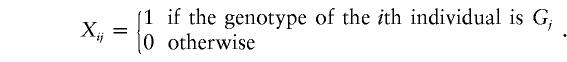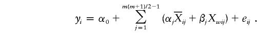
Following the definitions of , A_wi, and D_wi in the Methods section, we may similarly define and X_wij. We can then test the null hypothesis H₀:β₁=⋅⋅⋅=β_m(m+1)/2-1=0 through use of the following regression model:

In the present study, we have introduced a similarity indicator, W_ij, between the ith and the jth individuals from the t_ijk to characterize whether these two individuals are more likely to be from the same or from different subpopulations. An alternative approach to using the t_ijk values is to directly apply these estimated probabilities in the QSAT method; however, we have found that this approach is less powerful than that using the W_ij values (data not shown).

The QSAT proposed in this article involves the pooling of information from all subpopulations. If there are two subpopulations, allele A₁ increases trait values in one subpopulation, and another allele, A₂ increases trait values in another subpopulation, the QSAT may lose power. An alternative method is to directly test the hypothesis H₀:α₁=…=α_k=0 and β₁=…=β_k=0 under the model in equation (3). To apply this procedure, we need to infer population structure through use of genomic markers—for example, by means of the procedure proposed by Pritchard et al. (2000b). There are two potential problems with this alternative approach: (1) the estimation procedure proposed by Pritchard et al. (2000b) tends to overestimate the number of subpopulations in a sample and (2) the degrees of freedom for the test statistic is 2k, where k is the number of estimated subpopulations, and a test statistic with many degrees of freedom may lose power. If the same allele increases trait values in all subpopulations, the QSAT is likely to be more powerful than this alternative testing procedure. If different alleles increase trait values in different subpopulations, the relative performance of the statistical tests needs further investigation.

Appendix A : The Expectation of and under the Model in Equation (3)

Suppose that there are k subpopulations, with n_i individuals sampled from the ith subpopulation. Let denote the total sample size, μ_i denote the phenotype mean in the ith subpopulation, and let p_i and q_i denote the allele frequencies in the ith subpopulation.

Under the model in equation (3), the LS estimators of α and β are

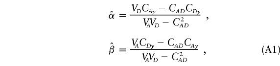where

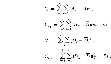and

From equation (2), we have

where

and

In the equation, α_(α)i, d_(α)i, a_(β)i, and d_(β)i are functions of A_ij and D_ij and satisfy the following conditions:

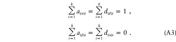If α₁=…=α_k=α^* and β₁=…=β_k=β^*, it follows from equations (A1), (A2), and (A3) that and . Furthermore, under the null hypothesis H₀:α₁=…=α_k=0 and β₁=…=β_k=0, and .

Let V=V_AV_D-C²_AD. For large values of n and n_i (i=1,…,k),

and

Through some calculations, we have

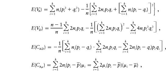and

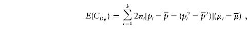where and . In the case of two subpopulations—that is, when k=2—and with an equal number of individuals from each subpopulation—that is, when n₁=n₂—we have

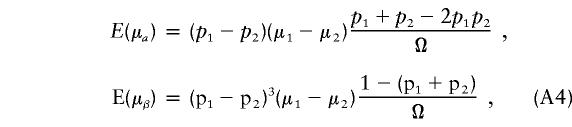where Ω=2(p₁q₁+p₂q₂)[(p₁q₁+p₂q₂)²+(p₁-p₂)²]. From equation (A4), we can see that if the phenotypic means and allele frequencies vary between subpopulations—that is, if μ₁≠μ₂ and p₁≠p₂—then E(μ_α)≠0. Furthermore, if p₁+p₂≠1, then E(μ_β)≠0.

Appendix B: The Expectations of , and under the Model in Equation (4)

Under the model in equation (4), the LS estimates of and are

and

where

and

Note that . Under the model in equation (2), we have

and

After some algebraic calculations, we obtain

and

where a_(α)i, d_(α)i, a_(β)i, and d_(β)i are functions of A_ij and D_ij and satisfy

and

If α₁=…=α_k=α^* and β₁=…=β_k=β^*, it follows that and . In this case, and are both unbiased estimators of the additive and dominance genetic values α* and β*, respectively. Even if the additive and dominance genetic values vary among subpopulations, we still have under the null hypothesis H₀.

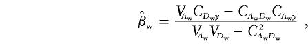
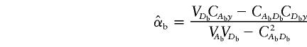
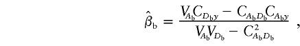
Under the model in equation (4), the LS estimates of and are given by

and

where

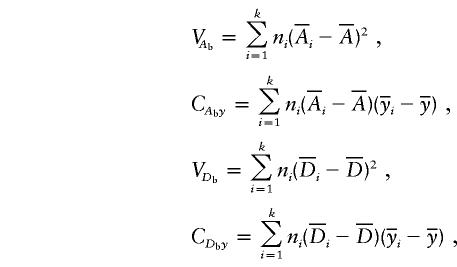and

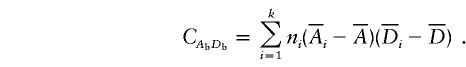It follows from the model in equation (2) that, after some algebraic calculations,

and

where

and

The variables a_(bα)i, d_(bα)i, a_(bβ)i, and d_(bβ)i are functions of A_ij and D_ij and satisfy

and

If α₁=…=α_k=α^* and β₁=…=β_k=β^*, it follows that and . Furthermore, under the null hypothesis α₁=…=α_k=0 and β₁=…=β_k=0, and .

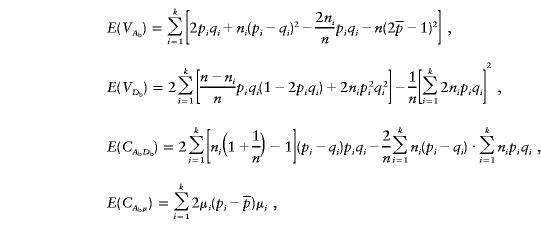
Let V_b=V_AbV_Db-C²_AbDb. For large values of n and n_i (i=1,…,k),

and

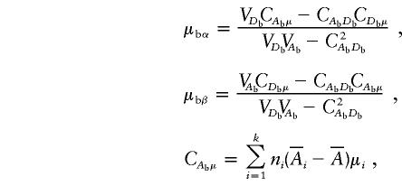
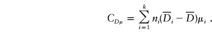
Therefore, we have

and

For k=2 and n₁=n₂, we have

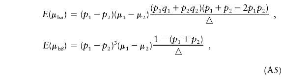where

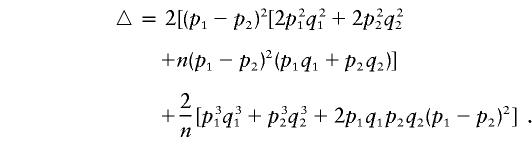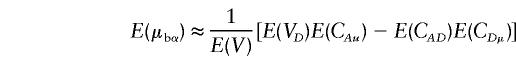
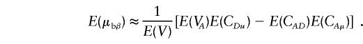
From equation (A5), we can see that if the phenotypic means and allele frequencies vary between the two subpopulations—that is, if μ₁≠μ₂ and p₁≠p₂—then E(μ_bα)≠0. Furthermore, if p₁+p₂≠1, then E(μ_bβ) ≠ 0.

References

- Abecasis GR, Cardon LR, Cookson OC (2000) A general test of association for quantitative traits in nuclear families. Am J Hum Genet 66:279–292 [DOI] [PMC free article] [PubMed] [Google Scholar]
- Bacanu SA, Devlin B, Roeder K (2000) The power of genomic control. Am J Hum Genet 66:1933–1944 [DOI] [PMC free article] [PubMed] [Google Scholar]
- Celeux G, Govaert G (1995) Gaussian parsimonious clustering model. Pattern Recognition 28:781–793 [Google Scholar]
- Devlin B, Roeder K (1999) Genomic control for association studies. Biometrics 55:997–1004 [DOI] [PubMed] [Google Scholar]
- Fulker DW, Cherny SS, Sham PC, Hewitt JK (1999) Combined linkage and association sib-pair analysis for quantitative traits. Am J Hum Genet 64:259–267 [DOI] [PMC free article] [PubMed] [Google Scholar]
- Goldstein DB, Linares AR, Cavalli-Sforza LL, Feldman NW (1995) Genetic absolute dating based on microsatellites and the origin of modern humans. Proc Natl Acad Sci USA 92:6723–6727 [DOI] [PMC free article] [PubMed] [Google Scholar]
- Griffiths RC, Tavaré S (1994) Ancestral inference in population genetics. Stat Sci 9:307–319 [Google Scholar]
- ——— (1997) Computational methods for the coalescent. In: Tavaré S, Donnelly P (eds) Progress in population genetics and human evolution. IMA Vol 87. Springer-Verlag, pp 165–182 [Google Scholar]
- Monks SA, Kaplan NL (2000) Removing the sampling restrictions from family-based tests of association for a quantitative-trait locus. Am J Hum Genet 66:576–592 [DOI] [PMC free article] [PubMed] [Google Scholar]
- Morton NE, Collins A (1998) Tests and estimates of allelic association in complex inheritance. Proc Natl Acad Sci USA 95:11389–11393 [DOI] [PMC free article] [PubMed] [Google Scholar]
- Osier MV, Cheung KH, Kidd JR, Pakstis AJ, Miller PL, Kidd KK (2001) ALFRED: an allele frequency database for diverse populations and DNA polymorphisms: an update. Nucleic Acids Res 29:317–319 [DOI] [PMC free article] [PubMed] [Google Scholar]
- Pritchard JK, Rosenberg NA (1999) Use of unlinked genetic markers to detect population stratification in association studies. Am J Hum Genet 65:220–228 [DOI] [PMC free article] [PubMed] [Google Scholar]
- Pritchard JK, Stephens M, Donnelly P (2000a) Inference of population structure using multilocus genotype data. Genetics 155:945–959 [DOI] [PMC free article] [PubMed] [Google Scholar]
- Pritchard JK, Stephens M, Rosenberg NA, Donnelly P (2000b) Association mapping in structured population. Am J Hum Genet 67:170–181 [DOI] [PMC free article] [PubMed] [Google Scholar]
- Reich EE, Goldstein DB (2001) Detecting association in a case-control study while correcting for population stratification. Genet Epidemiol 20:4–16 [DOI] [PubMed] [Google Scholar]
- Risch N (2000) Searching for genetic determinants in the new millennium. Nature 405:847–856 [DOI] [PubMed] [Google Scholar]
- Risch N, Merikangas K (1996) The future of genetic studies of complex human diseases. Science 273:1516–1517 [DOI] [PubMed] [Google Scholar]
- Risch N, Teng J (1998) The relative power of family-based and case-control designs for linkage disequilibrium studies of complex human diseases. I. DNA pooling. Genome Res 8:1273–1288 [DOI] [PubMed] [Google Scholar]
- Satten GA, Flanders WD, Yang Q (2001) Accounting for unmeasured population substructure in case-control studies of genetic association using a novel latent-class model. Am J Hum Genet 68:466–477 [DOI] [PMC free article] [PubMed] [Google Scholar]
- Sham PC, Cherny SS, Purcell S, Hewitt JK (2000) Power of linkage versus association analysis of quantitative traits, by use of variance-components models, for sibship data. Am J Hum Genet 66:1616–1630 [DOI] [PMC free article] [PubMed] [Google Scholar]
- Spielman RS, McGinnis RE, Ewens WJ (1993) Transmission test for linkage disequilibrium: the insulin gene region and insulin-dependent diabetes mellitus (IDDM). Am J Hum Genet 52:506–513 [PMC free article] [PubMed] [Google Scholar]
- Sun F, Flanders WD, Yang Q, Zhao HY (2000) Transmission/disequilibrium tests for quantitative traits. Ann Hum Genet 64:555–565 [DOI] [PubMed] [Google Scholar]
- Teng J, Risch N (1999) The relative power of family-based and case-control designs for linkage disequilibrium studies of complex human diseases. II. Individual genotyping. Genome Res 9:234–241 [PubMed] [Google Scholar]
- van den Oord EJCG (1999) A comparison between different designs and tests to detect QTLs in association studies. Behav Genet 29:245–256 [Google Scholar]
- Wang DG, Fan JB, Siao CJ, Berno A, Young P, Sapolsky R, Ghandour G, et al (1998) Large-scale identification, mapping, and genotyping of single-nucleotide polymorphisms in the human genome. Science 280:1077–1082 [DOI] [PubMed] [Google Scholar]
- Zhang SL, Kidd KK, Zhao HY. Detecting genetic association in case-control studies using similarity-based association tests. Statistica Sinica (in press) [Google Scholar]