Robust-tuning machine learning algorithms for precise prediction of permeability impairment due to CaCO₃ deposition

Abstract

Scale buildup, especially calcium carbonate (CaCO₃), is a common problem in Enhanced Oil Recovery (EOR) operations, often caused by injecting incompatible water or by changes in pressure and temperature that trigger chemical reactions. This buildup can clog reservoirs, damage wells, and affect surface equipment by reducing permeability. This study explores how factors like temperature, pressure, pH, and ion concentration influence CaCO₃ deposition and how it affects reservoir performance. Using machine learning models—Support Vector Regression (SVR), Extra Trees (ET), and Extreme Gradient Boosting (XGB)—the research aims to predict how much permeability is lost due to scaling. With proper tuning of these models, prediction accuracy significantly improved: SVR rose from 92 to 99.88%, and XGB reached 99.87%, while ET remained consistently high at around 99.98%. The real value of this work lies in building a fine-tuned, practical machine learning approach that applies proven models to real-world EOR challenges. Instead of creating new algorithms, the study focuses on refining existing ones to make them more effective for the field. These accurate predictions can help engineers make smarter decisions about maintaining wells and reservoirs, ultimately improving efficiency and cutting operational costs.

Introduction

When an oil reservoir is linked to the surface through drilling, some oil might naturally emerge due to the reservoir’s inherent pressure. This initial oil output, augmented by pumping from individual wells to support the natural flow, is termed primary oil recovery. Following primary extraction, the recovery rate typically remains low, usually below 25% of the original oil reserves. Various methods are employed to enhance oil retrieval, with water injection being a prevalent approach. Injection wells introduce treated seawater, brine, or reservoir water into the oil reservoir to uphold pressure or drive the oil toward production wells. This pressure maintenance technique is commonly known as secondary recovery or water flooding. Large volumes of water are injected into reservoirs to maintain reservoir pressure. This can lead to salt precipitation due to the composition of the injected water¹. As reservoir depletion progresses and water cuts in wells rise, the deposition issue exacerbates. Moreover, the extraction of residual oil necessitates applying advanced techniques encompassing both physical and chemical methodologies. These endeavors aim at enhancing oil recovery, consequently triggering and amplifying scale deposition^2,3. The scale represents a flow assurance challenge from deposition and chemical precipitation from dissolved compounds in reservoir water or water introduced into the reservoir during gas and oil extraction⁴. Various inorganic scales exist in oil fields, distinguished by their compositions. Among the prevalent deposits encountered are calcium carbonate (CaCO₃), calcium sulfate (CaSO₄), barium sulfate (BaSO₄), known for its extremely low solubility and consequent problematic nature, as well as strontium sulfate (SrSO₄), zinc sulfide (ZnS), lead sulfide (PbS), etc^5,6. The occurrence of deposits within pores and surface facilities arises from the saturation of the surrounding environment with mineral salts. The scale represents a significant challenge in the oilfield, exacerbating equipment corrosion and resulting in wellbore blockages and flow impediments. This leads to decreased oil and gas production and frequent shutdowns of wells and production equipment for the costly and time-intensive processes of well replacement and predrilling to mitigate plugged wells⁷. The primary cause of scale deposition typically stems from the injection fluid’s lack of compatibility with the reservoir^8,9. Such deposits pose significant risks to the formation integrity and can significantly diminish oil productivity and recovery rates. Given the growing complexity of enhanced oil recovery (EOR) operations and the economic consequences of scale deposition, particularly CaCO₃, there is an urgent need for predictive tools that can anticipate formation damage before it occurs.

A recent study by De Angelo et al.¹⁰ investigated the effect of steel surface roughness on CaCO₃ deposition in salt water with high salinity. This experiment was conducted on one of the reservoirs in Brazil, which has the problem of high levels of carbon dioxide (CO₂) in the accompanying gas, high water salinity, and high concentration of calcium ions. The results of this work indicate that smoother surfaces have less adhesion to calcium carbonate than surfaces with higher roughness, and surface roughness affects calcium carbonate polymorphs related to the corrosion process. The formation of BaSO₄ is minimally affected by higher salinity under varying pressures. Typically, the precipitation of salt results in the generation of solid, suspended particles due to the clustering of crystals^11,12. Schmid et al.¹³ studied the deposition challenges of Montney oil fields. The presence of radioactive materials (NORM) in sediments leads to health problems and disposal costs. Also, due to the horizontal structure and multiple fractures of the Montney reservoirs, conventional sediment inhibitors only reach the production area partially. This study presented a method for injecting sediment inhibitors into these fields using modeling and various experiments. The results show that injecting a sediment inhibitor increases pump life, removes NORM from surface equipment, reduces the need for acid washing, and reduces production stoppages. In their research, Khormali et al. concentrated on developing a novel sediment inhibitor tailored to impede calcium carbonate formation across three distinct synthetic formation waters. Fine-tuning the concentration of hydrochloric acid within the inhibitor was determined through surface tension measurements at the oil-aqueous solution interface. Findings reveal that the optimal mass percentage of a 5% hydrochloric acid solution within the inhibitor is 8 to 10%. Additionally, augmenting the concentration of organic components to decrease surface tension markedly curtails CaCO₃ precipitation. Furthermore, variations in flow rate influence the induction period of crystallization, a pivotal aspect in scale management strategies^14,15. Zhang’s exploration into the co-precipitation of calcium carbonate and barium carbonate under typical oil field operation conditions shed light on the substantial impact of saturation levels and Ca/Ba molar ratios on the co-precipitation process. These insights offer valuable guidance for scale formation management strategies¹⁶. As depicted in Fig. 1, scale formation is contingent upon numerous parameters, including pressure, temperature, pH levels, flow velocity, impurities and carbon dioxide, agitation and turbulence during crystal formation, the size and quantity of seed crystals, and the degree of super-saturation^17–19. To manage scale deposition, the researchers investigated the deposition and scaling processes of CaCO₃ under varying temperature and salinity conditions. Additionally, they explored the impact of organic chelating agents on the dissolution and separation of CaCO₃ in high-salinity environments. Temperature and salinity significantly influence the formation of CaCO₃ precipitates, with elevated temperatures prompting the transformation of vaterite CaCO₃ into aragonite or calcite CaCO₃, a process accelerated by the presence of salt²⁰. As another EOR scenario, in the ASP flooding process, precipitates primarily consist of carbonates and silicates. An increase in pH enhances silicate content while reducing carbonate concentration, whereas silicon ions accelerate calcium precipitation. Additionally, higher concentrations of calcium and magnesium ions facilitate precipitation; however, magnesium precipitates only after the chemical equilibrium of calcium and barium is established²¹. Moreover, an increase in temperature (from 45 °C to 80 °C) promotes silicate and aluminum precipitation, while a rise in pressure (from 0.1 MPa to 1.4 MPa) increases the concentrations of calcium and magnesium in the solution²².Beyond the mentioned cases, the ASP flooding in the Daqing oilfield, China, resulted in reservoir damage, with varying severity depending on well locations. The formation damage differed across areas near injection and production wells, influencing the efficiency of oil recovery²³. As a result, in addition to water injection, ASP injection also leads to severe damage to the formation.

Fig. 1.

Factors influencing scale precipitation and followed steps during CaCO₃ scale deposition²⁴.

Modeling scale buildup and predicting the extent of formation damage caused by scale

Given the limitations of traditional experimental approaches in identifying complex, nonlinear relationships between scale-forming parameters, the use of artificial intelligence (AI) and machine learning (ML) is becoming increasingly relevant. Adopting machine learning and deep learning, integral components of artificial intelligence algorithms has emerged as a prevalent practice within the oil and gas sector (Fig. 2). Recent investigations underscore the promising utility of artificial intelligence methodologies in predicting reservoir parameters and assessing reservoir damage. Within these studies, artificial neural networks (ANN) are often leveraged to forecast permeability and characterize the type and quantity of sediment formation, provided relevant data is accessible.

Fig. 2.

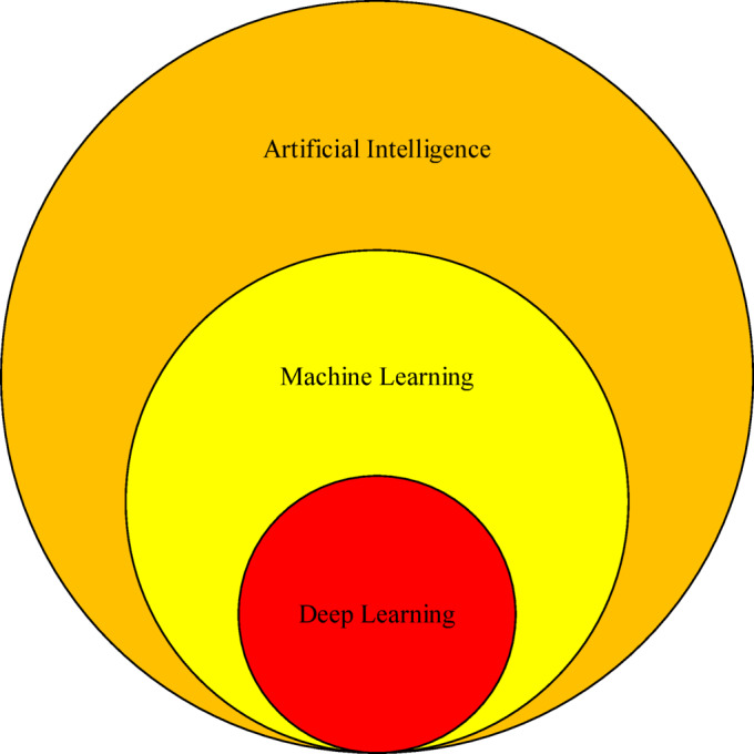
Machine learning and deep learning are a subset of artificial intelligence.

In predicting permeability within porous media, particularly in hydrocarbon reservoirs, Tahmasebi conducted research focused on crafting a rapid and autonomous neural network. This neural network is adept at swiftly analyzing data and generating predictions with minimal human intervention. Validation was performed using real-world data from oil and gas reservoirs to ascertain the model’s accuracy and dependability²⁵. Utilizing neural network models to explore sedimentation challenges in reservoirs and wells and develop a predictive model for assessing the risk of sound blockage and evaluating preventive measures within the reservoir offers a comprehensive understanding of CaCO₃ sedimentation. It is well understood that Temperature fluctuations mainly influence CaCO₃ precipitation²⁶. In 2014, Zabihi and colleagues conducted a comparative analysis of two back-propagation learning algorithms alongside Levenberg-Marquardt, utilizing well-drilling data from clayey sandstone reservoirs. This investigation underscores artificial neural networks’ capability to surpass traditional statistical approaches’ constraints, particularly in permeability estimation²⁷. In 2019 and 2020, Al-Hajri predicted calcium carbonate scale formation and developed control strategies for oil well applications involving utilizing machine learning models like Support Vector Machines (SVM) and k-nearest Neighbors (KNN). Key data inputs included ionic composition, pH levels, sampling/inspection dates, and records of scale formation incidents. These endeavors culminated in highly accurate deposit forecasts, boasting a 95% accuracy rate, and yielded cost savings threefold more significant than current programs^28,29. In complement to established algorithms, the approach involves constructing an experimental model for sediment formation rates employing artificial intelligence techniques. This model considers pressure, temperature, fluid velocity, and saline concentration factors. For instance, in 2016, Hamid and colleagues introduced an experimental methodology for forecasting the potential rate of CaCO₃ deposition in well completions, particularly emphasizing smart well completions³⁰. In the background research and studies conducted in 2022, an investigation focused on the thermodynamic and compositional attributes of well water samples containing deposits of BaSO₄ and CaCO₃. This examination incorporated parameters such as temperature, pressure, molar fraction of CO₂, total dissolved solids (TDS), and water ionic composition. Logistic regression algorithms, support vector classifier (SVC), and decision tree classifier methodologies were employed. Notably, the decision tree classifier demonstrated superior accuracy, achieving an accuracy level of 0.91³¹. In a recent study led by Yousefzadeh et al.³², machine-learning methods were applied to forecast scale precipitation occurrences and their impacts on oilfield equipment. Additionally, the study carried out a sensitivity analysis to identify the key factors affecting scale formation. The findings indicate that KNN and ensemble learning methods were the most accurate, demonstrating outstanding effectiveness in distinguishing between scale and no-scale scenarios. Nallakukkala’s et al. research³³ showcases the utilization of machine learning to forecast scale buildup within the oil and gas industry. This study delves into scale origins, deposition mechanisms, and strategies for controlling scale formation. In 2024, Khodabakhshi and Bijani³⁴, researched sulfate scale deposits like BaSO₄, SrSO₄, and CaSO₄, focusing on forecasting reservoir permeability reduction using machine learning techniques. The study employed several algorithms, including SVR, RF, and XGB, among others, and emphasized the significance of hyperparameter optimization. The KNN and XGB algorithms achieved a high accuracy of 0.996 in predicting permeability loss, although KNN exhibited significantly lower error indices than XGB. Despite this, both algorithms demonstrated equal precision in identifying permeability reduction. Studies have also been conducted to predict the effect of ASP on permeability loss and scale deposition risk reduction. A data-mining-based model has achieved an accuracy of 91.87% in predicting ionic variations and scale formation³⁵. Additionally, the application of the Particle Swarm Optimization (PSO) method has been proposed to minimize chemical costs and reduce the risk of scale deposition in the ASP process³⁶. The machine learning model developed in this study can be directly applied in real-world oilfield operations to predict calcium carbonate (CaCO₃) scaling risks using real-time data such as temperature, pressure, and ion concentrations. In a typical water injection setup, this model helps field engineers identify high-risk wells early, prioritize chemical treatments, and adjust injection parameters to prevent scale buildup—similar to practices used in challenging environments like sour, high-temperature reservoirs³⁷. For instance, when the model signals a high scaling potential, operators can take proactive steps like fine-tuning the water chemistry³⁸, planning timely maintenance³⁹, or applying scale inhibitors to specific wells. This shifts field management from reacting to scale problems to actively preventing them. The approach builds on proven workflows, including thermodynamic and kinetic modeling⁴⁰, dynamic flow simulations in pipelines⁴¹, and even advanced virtual sensors that forecast scale risks in real time⁴².

The accumulation of CaCO₃ deposits in oil and gas reservoirs is not only a geochemical concern but also an economic and operational challenge. It leads to formation damage, increased maintenance costs, and reduced reservoir productivity. The research gap observed in previous works is the need for sufficient attention to the effect of the formation of carbonate sediments on the reduction of permeability as formation damage. Previous research has been mainly based on laboratory tests and limited work on predicting the effect of scaling on reservoir permeability. In this current study, a large data set was used, which was the output of original flood experiments with many features. The novelty and industrial relevance of this study lie in its application of advanced, tuned machine learning algorithms to predict permeability loss from CaCO₃ scaling under real-world reservoir conditions. This approach offers significantly improved accuracy and reliability compared to previous research. First, the study utilizes a large and diverse dataset derived from real-world field and laboratory experiments, encompassing actual operational conditions in petroleum reservoirs. Unlike prior studies that primarily relied on numerical simulations or limited datasets, this research incorporates a wide range of environmental variables that influence CaCO₃ precipitation and permeability reduction. Second, by leveraging multiple machine learning algorithms, this study enhances the precision and reliability of permeability predictions, facilitating direct applications in reservoir management and production optimization. This methodology not only improves the accuracy of machine learning models but also provides a deeper understanding of the mechanisms underlying permeability impairment, thereby contributing to the development of effective mitigation strategies for scaling-related damage. Ultimately, the findings of this research offer significant benefits to the oil and gas industry. The proposed models enhance permeability prediction, aiding in resource estimation, production planning, and the formulation of preventive maintenance strategies. Furthermore, this study opens new horizons in applying machine learning for the precise forecasting of permeability impairments and optimizing water injection processes in petroleum reservoirs—an area that has received limited attention to date.

Methodology

Figure 3 shows a schematic for the process adopted in this study, from the data acquisition to determining the best model.

Fig. 3.

Flowchart of the methodology.

Machine learning

Machine learning is a type of artificial intelligence that involves building computer systems that improve through experience and understanding the basic rules governing learning systems. These algorithms were developed to meet the demands of computationally tractable algorithms for massive data sets and algorithms that minimize privacy effects⁴³. On the other hand, due to recent developments in information recording technologies, there is a large amount of data in the oil and gas industry, and machines analyze this extensive data⁴⁴.

Support vector machine algorithm

Support vector regressor (SVR), introduced by Vapnik and colleagues in the 1960s, are a machine learning technique grounded in statistical learning theory and the principle of structural risk minimization^45,46. SVR are highly dependable and function by creating a dividing line or hyperplane to segregate labeled datasets. The algorithm aims to identify the line that maximizes the separation between two labeled datasets, establishing the most significant possible margin. This characteristic contributes to the algorithm’s high accuracy⁴⁷. The algorithm’s schematic is illustrated in Fig. 4.

Fig. 4.

Diagram illustrating the support vectors with an error margin of ϵ.

Decision tree algorithm

Decision trees DT are valuable in machine learning. Their widespread adoption is driven by their straightforwardness, ease of interpretation, visual representation, and minimal computational expense. DT enable the depiction of algorithms through conditional control statements, with branches illustrating decision points that guide toward a target result. Figure 5 illustrates the schematic of this algorithm. The hierarchical structure comprises a series of conditions or constraints extending from the root node to the terminal node (leaf)^48,49.

Fig. 5.

Conceptual depiction of a decision tree.

Random forest algorithm

Random forest (RF) combines multiple DT algorithms to predict or classify a variable’s value. In RF, each tree contributes to a single, more precise prediction by casting one vote^50–52. Figure 6 displays the schematic of this algorithm. Ensemble learning algorithms generally offer greater robustness and accuracy than individual classifiers or regressors^53,54.

Fig. 6.

Structure of a random forest⁵⁵.

Extra tree algorithm

Geurts and colleagues initially introduced Extra Trees (ET), also referred to as highly randomized trees⁵⁶. This algorithm enhances the RF method, designed to reduce the likelihood of overfitting. In ET and RF, each base estimator is trained on a randomly selected subset of features. The algorithm’s schematic is illustrated in Fig. 7. The primary goal of the ET algorithm is to lower the prediction model’s variance by implementing more advanced randomization techniques.

Fig. 7.

Extremely randomized trees schematic⁵⁷.

Gradient boost algorithm

As one of the machine learning algorithms, gradient boosting algorithms act like a team that learns from its mistakes, which is the difference between boosting and bagging algorithms (Fig. 8). These algorithms will use the ensemble method, meaning they start with a series of simple models that are then refined and improved at each step to create a robust predictive model^58,59.

Fig. 8.

The difference between learning in bagging and boosting mode⁶⁰.

XG boost algorithm

XGBoost is one of the most powerful and widely-used machine learning algorithms. Its optimized implementation allows for high accuracy with large datasets. The algorithm employs the boosting technique, where weak learners (decision trees) are developed in sequence. Each new tree focuses on the prediction errors made by the previous tree. This process combines the weak learners into a strong model, ensuring robust performance⁶¹. The diagram of this algorithm is depicted in Fig. 9.

Fig. 9.

Extreme gradient boosting algorithm technique⁶².

K-nearest neighbor

The KNN algorithm, originally created by Fix⁶³ and later refined by Cover and Hart⁶⁴, is a nonparametric method that relies on similarity measures. Figure 10 illustrates the schematic of this algorithm. It identifies the k nearest neighboring points within the sample data using these measures. The algorithm predicts the output category by determining the most common class among the k neighbors.

Fig. 10.

KNN technique with different neighbors.

Data preparation

Data preparation is the process of preparing raw data for post-processing and analysis. The essential methods are collecting, cleaning, and labeling the raw data into a format suitable for machine learning (ML) algorithms, followed by data exploration and visualization⁶⁵. This part of this study includes data gathering, data normalization, removing outliers, a heat map, and a pair plot, which are explained below.

Data gathering

Data related to core flooding tests have been collected to carry out this research. The number of recorded data is 900, and its characteristics are listed in Table 1. These data are obtained from tests performed in different conditions. They can be used to analyze the behavior of fluid and rock during the water injection process in oil and gas reservoirs.

Table 1.

Data extracted from the core flood test.

	Pressure drop	Temperature	Ca (ppm)	HCO3 (ppm)	Q (cc/min)	pH	CO2 partial pressure	Permeability ratio
Count	899	899	899	899	899	899	899	899
Mean	7746.563	58.865	2530.634	1139.421	52.641	5.950	253959.955	0.566
Std	7614.213	11.16	558.546	253.802	19.723	0.091	59223.845	0.273
Min	1164.788	50	1770	800	25	5.88	130,000	0.101
25%	3037.824	50	2360	1060	50	5.88	200,000	0.303
50%	4682.62	50	2360	1060	50	5.88	300,000	0.6
75%	9271	70	2360	1060	50	6.03	300,000	0.798
Max	46069.584	80	3540	1600	100	6.15	300,000	1.067

Data normalization

Data normalization is one of the most vital steps for data preparation, which leads to more accurate model predictions. This method converts the current data range to a new standard range between 0 and 1. Normalization aims to find a standard scale for the data while preserving the inherent variation in the range of values⁶⁶. Table 2 contains the types of normalization methods.

Table 2.

Type of data scaling⁶⁰.

Method	Equation	Description
Normalization (Min–Max scaler)		Normalization scales the values of a feature to a specific range, often between 0 and 1, and maintains the shape of the original distribution, susceptible to the influence of outliers.
Standardization (Z-score)		Standardization scales the features to have a mean of 0 and a standard deviation of 1, alters the shape of the original distribution, and is less affected by the presence of outliers; is the mean of data, and is the standard deviation.

Removing outliers and noisy data

In machine learning, random or irrelevant data, known as noise, can lead to unpredictable situations that differ from what is expected. Incorrect measurements, data collection, or irrelevant information cause this⁶⁷. An outlier is a data item/object that deviates significantly from the other objects (so-called normal). Identifying outliers is vital in statistics and data analysis because they can significantly impact the results of statistical analyses. Analysis to detect outliers is called outlier extraction. Outliers can skew the mean (average) and affect measures of central tendency, as well as affect the results of tests of statistical significance⁶⁸.

Heat map

A heat map is a graphical representation of data that uses colors to visualize the matrix’s value. It is often used to visualize a dataset’s correlation or relationships between different variables⁶⁹. In a heat map, each cell’s color intensity corresponds to the value it represents, allowing for a quick and intuitive assessment of patterns or relationships within the data.

Pair plot

A pair diagram, also known as a scatter matrix, is a matrix of diagrams that allows visualizing the relationship between any pair of variables in a data set. It combines histogram and scatter plot, providing a unique overview of the data set’s distributions and correlations⁷⁰. The primary purpose of the pairwise graph is to simplify the initial stages of data analysis by providing a comprehensive snapshot of the potential relationships within the data.

Algorithms model

After examining seven algorithms used in this study, the data underwent preprocessing to facilitate model comprehension. The prepared data was divided into training and test data at a ratio of 80:20. Machine learning models were trained with training data and tested with test data.

Tuning hyper-parameter

Grid search is a method for finding the best possible combination of meta-parameters for the highest accuracy of the model. Figure 11 depicts the operation of the grid search algorithm. To select the best combination, a model is tested with all possible combinations of hyperparameters on the validation set^71,72. Grid search can be applied to any hyperparameter algorithm whose performance can be improved by tuning the hyperparameter.

Fig. 11.

Procedure for grid search pattern technique⁷³.

Model evaluation

This research endeavored to examine the performance accuracy of algorithms using various metrics and achieve the maximum accuracy of each algorithm by tuning hyperparameters^55,74. Table 3 succinctly presents the parameters utilized to evaluate the performance of the algorithms.

Table 3.

Metrics used in the evaluation of models.

No.	Metric	Description	Formulas
1	MSE	In the context of regression analysis, MSE serves as a metric to quantify the average magnitude of deviations between predicted and observed values, obtained by squaring the differences.
2	RMSE	In regression analysis, RMSE serves as a common indicator of the typical prediction error. It’s calculated by taking the square root of the average squared differences between observed and estimated values.
3	MAE	Regression analysis can benefit from using MAE as a performance metric. MSE, MAE is less sensitive to the influence of outliers, offering a more robust measure of prediction discrepancy.
4	R-squared	In regression analysis, R-squared (coefficient of determination) captures the proportion of variance explained in the outcome variable.

Result and discussion

Data analysis

The extracted data were analyzed and prepared before being used to train machine learning models. The results of data preprocessing and analysis are as follows:

• The pressure drop data has outliers and must be cleaned; Fig. 12 shows the pressure drop box plot before removing the outliers, and Fig. 13 shows the pressure drop box plot after removing the outliers.

• Following outlier removal, duplicate points were eliminated, and the data index was reset. Min-max scaling was then applied to standardize the data and features to prevent algorithmic errors. The normalized data information is shown in Table 4.

• The grid, a visual representation, uses color intensity to depict the association between data pairs. Deeper blue hues indicate a strong inverse relationship, while green signifies neutrality. Conversely, deep green represents a powerful positive connection. By analyzing these color variations, the matrix provides valuable insights, facilitating the swift detection of interdependencies within the data’s various aspects.

• The heatmap diagram in Fig. 14 reveals a direct relationship between the Ca(ppm) and HCO₃(ppm) features. This suggests that removing one of these features could simplify the machine-learning process. However, they were retained due to the crucial role of both features, ensuring a comprehensive and robust machine-learning process.

• CO₂partial pressure has an inverse linear relationship with pH, as shown in the heatmap diagram in Fig. 14. The number − 1 indicates an inverse linear relationship, and the number 1 indicates a direct linear relationship.

• Temperature has almost a direct linear relationship with pH and an inverse linear relationship with CO₂ partial pressure. The pair plot diagram also confirms the heatmap diagram.

• A grid of scatter plots unveils relationships between data points (Fig. 15). Analysis of these visualizations facilitates the discovery of patterns and correlations across various data aspects. The diagonal histograms provide information on the individual distributions of each data feature.

Fig. 12.

Box plot for pressure drop before removing outlier.

Fig. 13.

Box plot for pressure drop after removing outlier.

Table 4.

Data information after normalization.

	Count	Mean	std	min	25%	50%	75%	max
Pressure drop	722	0.325	0.244	0	0.138	0.261	0.476	1
T	722	0.323	0.383	0	0	0	0.666	1
Ca (ppm)	722	0.38919	0.29395	0	0.33333	0.33333	0.333	1
HCO3 (ppm)	722	0.38351	0.29506	0	0.325	0.325	0.325	1
Q (cc/min)	722	0.320	0.242	0	0.333	0.333	0.333	1
PH	722	0.287	0.353	0	0	0	0.555	1
CO2 partial pressure	722	0.701	0.361	0	0.411	1	1	1
Permeability ratio	722	0.522	0.260	0	0.325	0.560	0.731	1

Fig. 14.

Heatmap shows the compare status of each feature with other features.

Fig. 15.

Pair plots show a matrix of graphs that enables the visualization of relationship between each pair of variables in a dataset.

Tuning models

After normalization, the number of data reached 722, of which 80%, about 578 data, were used for training the algorithms. With the remaining data, the algorithms used in this study were tested. At first, the primary mode of the algorithms was used for training, and the results of using these algorithms, which include accuracies and errors, are given in Table 5. To check the output of these algorithms better, before tuning the hyperparameters, Figs. 17 and 18 show these outputs on the graph. Figure 16a-g is the output of algorithms without tuning hyperparameters. This output shows that the algorithms have a good understanding of the data in the primary state. In the meantime, GB and SVR algorithms need to be understood more than others, as shown in Fig. 16a and f (Figs. 17 and 18).

Table 5.

Algorithm’s output before hyperparameter optimization.

	MSE	MAE	RMSE	Training accuracy	Testing accuracy
Support vector regressor	0.0046	0.0595	0.0687	0.9325	0.9247
Decision tree	0.0002	0.0084	0.0167	0.9999	0.9955
Random forest	0.0001	0.0068	0.0114	0.9995	0.9979
Extra tree	0.0000	0.0016	0.0042	0.9999	0.9997
Gradient boost	0.0004	0.0098	0.0209	0.9999	0.9930
Extreme gradient boost	0.0001	0.0079	0.105	0.9998	0.9982
K-nearest neighbor	0.0002	0.0084	0.162	0.9985	0.9957

Fig. 17.

Error values for the base state of the algorithms.

Fig. 18.

Accuracy of algorithms in understanding training and test data.

Fig. 16.

Output of algorithms with lone of best fit and R-squared value.

Sensitivity analysis

A sensitivity study targeted specific hyperparameters in analyzing algorithm performance. Specifically, Fig. 19 delves into SVR’s C and degree parameters. The upper section showcases training data performance, while the lower section focuses on test data. Notably, altering the degree parameter minimally affects algorithm understanding across both data sets. However, increasing C leads to an accuracy boost in data comprehension, peaking at a certain value where further increments yield no accuracy gain.

Fig. 19.

Investigation the performance of SVR algorithm against C and degree hyperparameters.

The GB algorithm was analyzed for its hyperparameters max_depth and n_estimators. Observing Fig. 20, training accuracy remained steady despite parameter adjustments. However, test data performance varied: as max_depth and n_estimators increased, accuracy initially dropped, then rose without reaching the initial level. For this algorithm, the optimal settings appear to be n_estimators below 60 and max_depth between 10 and 15.

Fig. 20.

Sensitivity analysis on gradient boost algorithm.

In Fig. 21, the performance of the XGBoost algorithm is displayed concerning subsample hyperparameters and n-estimators. Initially, elevating subsample and n-estimators values led to improved algorithm accuracy. Notably, the n-estimators parameter significantly influences algorithm performance, with accuracy rising alongside its increase. While the algorithm performed well on training data with increased hyperparameter values, its performance on test data requires enhancement, highlighting the need for hyperparameter optimization to address this issue.

Fig. 21.

Effect of n-estimators and subsamples on the performance of gradient boost algorithm.

The KNN algorithm’s performance is notably affected by the n-neighbors and leaf-size hyperparameters, as indicated in Fig. 22. As these parameters are heightened, there is a noticeable decline in the algorithm’s accuracy, resulting in elevated prediction errors and diminished operational efficiency.

Fig. 22.

Effect of hyperparameters on accuracy of KNN algorithm.

This analysis aims to identify the key parameters influencing the algorithm’s performance in this study. This investigation aims to enhance our understanding of how each algorithm performs relative to different hyperparameters, facilitating the selection of optimal ranges for grid search operations. By improving the grid search’s efficacy, each algorithm’s accuracy in predicting permeability loss is enhanced. This heightened accuracy enables the identification of suitable measures to prevent significant production rate declines post-scale deposition, allowing for proactive interventions before such issues arise.

Hyper-parameters optimization

In this phase, the hyperparameters of the algorithms employed in this research were fine-tuned using the grid search technique. Although the algorithms initially exhibited high accuracy, it may be tempting to assume that further hyperparameter tuning is unnecessary. However, optimizing these parameters is crucial to avoid overfitting and ensure optimal performance on new data samples. Following the hyperparameter adjustments and considering the factors mentioned above, the algorithms’ outputs are presented in Table 6. The detailed data in this table provides insights into the algorithm performance post-hyperparameter optimization. The ET algorithm demonstrates superior performance, while DT, GB, and KNN algorithms exhibit similar accuracies to ET on training data. However, ET’s accuracy decreases when applied to test data, highlighting the critical role of hyperparameters in achieving high accuracy and minimizing error rates. Figure 23a-g visually represents the output and accuracy of each tuned algorithm. Analyzing the discrepancy between training and prediction accuracies suggests that these algorithms appropriately fit the data and are balanced. A significant disparity between training and test accuracies and a high error rate indicates potential overfitting in algorithms. This stems from the algorithms’ precise comprehension of extracted data, alongside thorough data preparation and preprocessing. With this comprehensive understanding and effective hyperparameter optimization, these algorithms can generalize well to new data that aligns with the extracted dataset. Consequently, they can accurately calculate and predict permeability loss due to scale deposition with remarkable precision. The alteration in oil flow direction caused by permeability loss is a pivotal factor in reservoir characteristics. Accurately predicting this parameter is essential for devising effective reservoir management strategies, such as stimulation tactics and enhancing oil recovery. A precise prediction directly influences the selection of optimal strategies, ensuring their effectiveness and success in reservoir management⁷⁵. Figure 23a and f illustrate a substantial increase in accuracy for the GB and SVR algorithms post-hyperparameter optimization, emphasizing the significance of this process. Figure 24 details the reduction in errors across all algorithms following hyperparameter tuning. Notably, the SVR algorithm’s RMSE index experienced a slight increase despite its improved accuracy, likely due to its sensitivity to outliers. Figure 25 showcases the impressive accuracy achieved by these algorithms post-optimization, indicating their readiness for field development implementation.

Table 6.

Algorithm’s results after tuning hyperparameters.

	MSE	MAE	RMSE	Training accuracy	Testing accuracy
Support vector regressor	0.0000	0.0062	0.084	0.9989	0.9988
Decision tree	0.0001	0.0070	0.0112	0.9999	0.9980
Random forest	0.0000	0.0053	0.0099	0.9995	0.9984
Extra tree	0.0000	0.0014	0.0037	0.9999	0.9998
Gradient boost	0.0004	0.0098	0.0209	0.9999	0.9930
Extreme gradient boost	0.0000	0.0061	0.0085	0.9998	0.9988
K-nearest neighbor	0.0000	0.0031	0.0089	0.9999	0.9987

Fig. 23.

Algorithm output after hyperparameter optimization.

Fig. 24.

Algorithms error after tuning hyperparameters.

Fig. 25.

Algorithms accuracy after hyperparameter optimization.

Precisely forecasting permeability losses from scale deposition, a pressing concern for the oil and gas sector, holds immense importance as it directly impacts reservoir management, production projections, and operational effectiveness. This study showcases that machine learning techniques offer a superior, more precise avenue for permeability prediction than conventional methodologies.

Model evaluation by distribution plot

Utilizing distribution charts to assess machine learning models is crucial for gauging their performance and confirming their generalization ability. Figure 26 overlapping bell curves signify a normal distribution in both datasets, aligning well with the requirements of machine learning models. The uniformity in distributions suggests that the model is poised to deliver consistent results across new training and test data, mitigating the chances of overfitting.

Fig. 26.

Distribution of train and test data.

The efficacy of hyperparameter tuning is evident in the close match between predicted values and the target variable. Figure 27a-g underscores the models’ grasp of fundamental data patterns, enabling accurate predictions. Post-hyperparameter adjustment, the distribution plots showcase the models’ ability to capture key data features and predict outcomes with high precision, validating their reliability for real-world applications. These graphical representations are vital in validating machine learning models before deployment. Comparing accuracy and errors in output values, SVR, GB, and XGB algorithms exhibit minimal overlap, as seen in Fig. 27b, f, and g. This slight variance justifies the findings in Table 6. Figure 28 also compares algorithm accuracy pre- and post-hyperparameter optimization, aiding in identifying the best-performing algorithm in this study.

Fig. 27.

Distribution plot for algorithms after adjustment hyperparameters.

Fig. 28.

Comparison between accuracy of algorithms before and after adjustment of hyperparameters.

Conventional methods like well logs and core data analysis are costly and time-intensive for predicting permeability. This study highlights machine learning’s efficiency and accuracy in permeability prediction, offering a significant advantage to the oil and gas sector by minimizing uncertainty in this crucial aspect. This reduced uncertainty directly impacts water saturation estimation, flow unit deliverability, and volumetrics assessment. Furthermore, machine learning algorithms aid in pinpointing key input parameters affecting permeability, enabling targeted strategies to mitigate permeability loss from scale deposition. Integrating machine learning into permeability prediction enhances reservoir modeling accuracy and reliability, which is crucial for optimizing oil and gas production operations. This model can assist operators in determining optimal scheduling for well chemical cleaning, adjusting operational conditions (such as temperature and pressure), and selecting appropriate anti-scaling additives. Moreover, the model’s predictions can be utilized to develop monitoring and control protocols for continuously tracking permeability changes and implementing corrective measures at the early stages of scale formation. These findings have significant applications in reservoir management and operational cost reduction within the oil and gas industry.

Conclusions

The findings of this research are summarized as follows:

• Prior to hyperparameter optimization, the ET algorithm demonstrates superior performance with an accuracy of 0.9997 in predicting permeability loss, outperforming all other current algorithms.

• The SVR method exhibits the least accuracy among the current algorithms, scoring 0.9247 in its predictions.

• While the KNN algorithm shows minimal error measures, its RMSE notably surpasses other algorithms, suggesting potential variance in model predictions.

• Ensemble techniques like RF, DT, GB, XGB, and ET demonstrate outstanding performance, exhibiting minimal error metrics and impressive accuracy.

• Following hyperparameter tuning, the SVR algorithm shows the most significant improvement among the algorithms examined, with its accuracy value rising by 8.0134%.

• Post hyperparameter tuning, the KNN algorithm saw its accuracy surge from 0.9957 to 0.9987, accompanied by a 94.5% reduction in its RMSE index value.

• Adjusting hyperparameters has generally enhanced the performance across all algorithms, which is particularly evident in the robust outcomes of ET, SVR, and XGB.

• The decision tree exhibits exceptional performance, boasting a 99.8% accuracy rate and minimal error. This model proves valuable for discerning the significance of various properties and can articulate clear decision rules elucidating how different factors impact permeability.

• Random forest, achieving a remarkable 99.84% accuracy, outperforms a decision tree in terms of generalization to unseen data. This enhanced generalization capability is crucial for accommodating the dynamic conditions often encountered in oil fields.

• Despite exhibiting a higher error rate than other models, Gradient Boost maintains an accuracy of 0.9930. This underscores the algorithm’s potency, particularly in capturing intricate nonlinear relationships.

• With an impressive accuracy of 0.9988, the XGB algorithm demonstrates outstanding performance, making it highly effective for forecasting tasks in the oil and gas industry. Its precision is crucial in sensitive situations, enabling accurate forecasting to drive optimization operations and significantly save costs.

• The real strength of this study lies not in creating a brand-new algorithm, but in customizing and fine-tuning proven machine learning models to tackle a complex, real-world problem in reservoir engineering. By carefully integrating data, optimizing model performance, and validating across several techniques, this framework offers a practical, reliable tool for field engineers. It helps them stay ahead of scale-related damage, streamline maintenance, and avoid costly downtime during Enhanced Oil Recovery (EOR) operations.

• These algorithms’ remarkable accuracy and minimal error rates highlight their effectiveness in predicting permeability loss caused by scale deposition. This capability enables more informed decision-making within the oil and gas sector, facilitating well-maintenance and extraction optimization. Ultimately, this leads to heightened efficiency and decreased operating costs.

For future research, we recommend exploring novel machine-learning techniques and conducting in-depth analyses of individual data points. Implementing deep learning algorithms, such as artificial neural networks, and comparing their predictive accuracy with existing methods could provide valuable insights. Additionally, incorporating data on pore structure and fluid properties—key indicators of sediment deposition’s effect on permeability—would enhance model reliability. To further improve generalizability and predictive accuracy, high-resolution numerical simulations should be conducted alongside complementary laboratory experiments. Extending this model for applications related to chemical EOR methods, including ASP flooding, is also crucial. Integrating additional data on chemical composition and the specific conditions of these techniques would refine predictions and enhance practical applicability. Furthermore, optimization strategies should be explored to improve algorithm adaptability with diverse data sources. Lastly, the impact of deposition-related damage on oil and gas production should be quantified by estimating production reduction and associated repair costs.

Abbreviations

CaCO₃

Calcium carbonate

HCO₃⁻

Bi-carbonate

ANN

Artificial neural network

SVR

Support vector regressor

AI

Artificial intelligence

ET

Extra tree

RF

Random forest

DT

Decision tree

KNN

K-Nearest neighbors

GB

Gradient boost

XGB

XG boost

TDS

Total dissolved solids

∆P

Pressure reduction

MSE

Mean squared error

MAE

Mean absolute error

RMSE

Root mean squared error

Author contributions

Mohammad Javad Khodabakhshi writing-original draft, methodology, conceptualization, performed the programming, contributed in analysis, and interpretation. Masoud Bijani supervised the project and contributed in writing and editing, data curation, reviewing the manuscript, and conceptualization. Masoud Hasani writing-original draft, methodology, and conceptualization.

Data availability

The datasets used and/or analyzed during the current study available from the corresponding author or reasonable request.

Declarations

Competing interests

The authors declare no competing interests.

References

- 1.Fan, C. et al. Scale prediction and Inhibition for oil and gas production at high temperature/high pressure. SPE J.17 (02), 379–392 (2012). [Google Scholar]
- 2.Awan, M. & Al-Khaledi, S. Chemical treatments practices and philosophies in oilfields. in SPE international oilfield corrosion conference and exhibition. SPE. (2014).
- 3.Demadis, K. D., Stathoulopoulou, A. & Ketsetzi, A. Inhibition And Control Of Colloidal Silica: Can Chemical Additives Untie The Gordian Knot Of Scale Formation? in NACE CORROSION. NACE. (2007).
- 4.Nassivera, M. & Essel, A. Fateh field sea water injection-water treatment, corrosion, and scale control. in SPE Middle East Oil and Gas Show and Conference. SPE. (1979).
- 5.Nwonodi, C. Prediction and Monitoring of Scaling in Oil Wells44 (Undergraduate Project, University of Port Harcourt, Rivers State, 1999).
- 6.Bijani, M., Behbahani, R. M. & Moghadasi, J. Predicting scale formation in wastewater disposal well of Rag-e-Safid desalting unit 1. Desalination Water Treat.65, 117–124 (2017). [Google Scholar]
- 7.Moghadasi, J. et al. Scale Formation in Oil Reservoir and Production Equipment during Water Injection Kinetics of CaSO4 and CaCO3 Crystal Growth and Effect on Formation Damage. in SPE European Formation Damage Conference. (2003).
- 8.Bijani, M., Khamehchi, E. & Shabani, M. Optimization of salinity and composition of injected low salinity water into sandstone reservoirs with minimum scale deposition. Sci. Rep.13 (1), 12991 (2023). [DOI] [PMC free article] [PubMed] [Google Scholar]
- 9.Bijani, M., Khamehchi, E. & Shabani, M. Comprehensive experimental investigation of the effective parameters on stability of silica nanoparticles during low salinity water flooding with minimum scale deposition into sandstone reservoirs. Sci. Rep.12 (1), 16472 (2022). [DOI] [PMC free article] [PubMed] [Google Scholar]
- 10.de Angelo, J. F. & Ferrari, J. V. Study of calcium carbonate scaling on steel using a high salinity Brine simulating a pre-salt produced water. Geoenergy Sci. Eng.233, 212541 (2024). [Google Scholar]
- 11.Bijani, M. & Khamehchi, E. Optimization and treatment of wastewater of crude oil desalting unit and prediction of scale formation. Environ. Sci. Pollut. Res.26 (25), 25621–25640 (2019). [DOI] [PubMed] [Google Scholar]
- 12.Jordan, M. M., Johnston, C. J. & Robb, M. Evaluation Methods for Suspended Solids and Produced Water as an Aid in Determining Effectiveness of Scale Control both Downhole and Topside21p. 7–18 (SPE Production & Operations, 2006). 01.
- 13.Schmid, J. et al. Mitigating Downhole Calcite and Barite Deposition in the Montney: A Successful Scale Squeeze Program. in SPE Canadian Energy Technology Conference. SPE. (2024).
- 14.Khormali, A. & Petrakov, D. G. Laboratory investigation of a new scale inhibitor for preventing calcium carbonate precipitation in oil reservoirs and production equipment. Pet. Sci.13, 320–327 (2016). [Google Scholar]
- 15.Khormali, A., Petrakov, D. G. & Moein, M. J. A. Experimental analysis of calcium carbonate scale formation and Inhibition in waterflooding of carbonate reservoirs. J. Petrol. Sci. Eng.147, 843–850 (2016). [Google Scholar]
- 16.Zhang, Z. et al. Laboratory Investigation of co-precipitation of CaCO3/BaCO3 Mineral Scale Solids at Oilfield Operating Conditions: Impact of Brine Chemistry75p. 83 (Oil & Gas Science and Technology–Revue d’IFP Energies nouvelles, 2020).
- 17.MacAdam, J. & Jarvis, P. Water-formed Scales and Deposits: Types, Characteristics, and Relevant Industries, in Mineral Scales and Depositsp. 3–23 (Elsevier, 2015).
- 18.Tungesvik, M. The Scale Problem, Scale Control and Evaluation of Wireline Milling for Scale Removal (University of Stavanger, 2013).
- 19.Yap, J. et al. Removing iron sulfide scale: a novel approach. in Abu Dhabi International Petroleum Exhibition and Conference. SPE. (2010).
- 20.Li, X. et al. Study on the scale Inhibition performance of organic chelating agent aided by surfactants on CaCO3 at high salinity condition. Tenside Surfactants Detergents, 2024(0).
- 21.Qing, G. Scaling Formation Characteristics of Ca~(2+)/Mg~(2+)/Si~(4+)/Ba~(2+) in ASP Flooding (Oilfield Chemistry, 2012).
- 22.Xian, W. An Experimental Study on Rock/Water Reactions for Alkaline/Surfactant/Polymer Flooding Solution Used at Daqing (Oilfield Chemistry, 2003).
- 23.Li, Z. et al. Formation damage during alkaline-surfactant-polymer flooding in the Sanan-5 block of the Daqing oilfield, China. J. Nat. Gas Sci. Eng.35, 826–835 (2016). [Google Scholar]
- 24.Trujillo-Chavarro, Y. C. et al. A Novel Integrated Methodology for Predicting and Managing Caco3 Scale Deposition in Oil-Producing Wells. Available at SSRN 4552032.
- 25.Tahmasebi, P. & Hezarkhani, A. A fast and independent architecture of artificial neural network for permeability prediction. J. Petrol. Sci. Eng.86, 118–126 (2012). [Google Scholar]
- 26.Su, X. et al. Research on the scaling mechanism and countermeasures of tight sandstone gas reservoirs based on machine learning. Processes12 (3), 527 (2024). [Google Scholar]
- 27.Zabihi, R., Schaffie, M. & Ranjbar, M. The prediction of the permeability ratio using neural networks. Energy Sour. Part A Recover. Utilization Environ. Eff.36 (6), 650–660 (2014). [Google Scholar]
- 28.Al-Hajri, N. M. & AlGhamdi, A. Scale Prediction and Inhibition Design Using Machine Learning Techniques. in SPE Gas & Oil Technology Showcase and Conference. SPE. (2019).
- 29.Al-Hajri, N. M. et al. Scale-prediction/inhibition design using machine-learning techniques and probabilistic approach. SPE Prod. Oper.35 (04), 0987–1009 (2020). [Google Scholar]
- 30.Hamid, S. et al. A practical method of predicting calcium carbonate scale formation in well completions. SPE Prod. Oper.31 (01), 1–11 (2016). [Google Scholar]
- 31.Ugoyah, J. C. et al. Prediction of Scale Precipitation by Modelling its Thermodynamic Properties using Machine Learning Engineering. in SPE Nigeria Annual International Conference and Exhibition. SPE. (2022).
- 32.Yousefzadeh, R. et al. An Insight into the Prediction of Scale Precipitation in Harsh Conditions Using Different Machine Learning Algorithms38p. 286–304 (SPE Production & Operations, 2023). 02.
- 33.Nallakukkala, S. & Lal, B. Machine Learning for Scale Deposition in Oil and Gas Industry, in Machine Learning and Flow Assurance in Oil and Gas Productionp. 105–118 (Springer, 2023).
- 34.Khodabakhshi, M. J. & Bijani, M. Predicting scale deposition in oil reservoirs using machine learning optimization algorithms. Results Eng., : p. 102263. (2024).
- 35.Hu, Y. & Lv, M. Research on prediction model of scaling in ASP flooding based on data mining. J. Comput. Methods Sci. Eng.23, 3037–3054 (2023). [Google Scholar]
- 36.Vazquez, O. et al. Optimization of Alkaline-Surfactant-Polymer (ASP) flooding minimizing risk of scale deposition. 2017: pp. 1–20. (2017).
- 37.Ness, G. et al. Application of a Rigorous Scale Prediction Workflow to the Analysis of CaCO3 Scaling in an Extreme Acid Gas, High Temperature, Low Watercut Onshore Field in Southeast Asia. in ADIPEC. (2022).
- 38.Amiri, M., Moghadasi & J. and The prediction of calcium carbonate and calcium sulfate scale formation in Iranian oilfields at different mixing ratios of injection water with formation water. Pet. Sci. Technol.30 (3), 223–236 (2012). [Google Scholar]
- 39.de Cosmo, P. Modeling and validation of the CO2 degassing effect on CaCO3 precipitation using oilfield data. Fuel310, 122067 (2022). [Google Scholar]
- 40.Zhang, Y. et al. The kinetics of carbonate scaling—application for the prediction of downhole carbonate scaling. J. Petrol. Sci. Eng.29 (2), 85–95 (2001). [Google Scholar]
- 41.Lai, N. et al. Calcium carbonate scaling kinetics in oilfield gathering pipelines by using a 1D axial dispersion model. J. Petrol. Sci. Eng.188, 106925 (2020). [Google Scholar]
- 42.Poletto, V. G. et al. Calcium Carbonate Formation within the Oil and Gas Workflow: A Combined Thermodynamic, Kinetic and CFD Modeling Approach. in Offshore Technology Conference Brasil. (2023).
- 43.Jordan, M. I. & Mitchell, T. M. Machine learning: trends, perspectives, and prospects. Science349 (6245), 255–260 (2015). [DOI] [PubMed] [Google Scholar]
- 44.Mohammadpoor, M. & Torabi, F. Big data analytics in oil and gas industry: an emerging trend. Petroleum6 (4), 321–328 (2020). [Google Scholar]
- 45.Vapnik, V. & Chervonenkis, A. On the one class of the algorithms of pattern recognition. Autom. Remote Control. 25 (6), 250 (1964). [Google Scholar]
- 46.Vapnik, V. N. Pattern recognition using generalized portrait method. Autom. Remote Control. 24 (6), 774–780 (1963). [Google Scholar]
- 47.Al-Anazi, A. F. & Gates, I. D. Support vector regression for porosity prediction in a heterogeneous reservoir: A comparative study. Comput. Geosci.36 (12), 1494–1503 (2010). [Google Scholar]
- 48.Breiman, L. Classification and Regression Trees (Routledge, 2017).
- 49.Patel, N. & Upadhyay, S. Study of various decision tree pruning methods with their empirical comparison in WEKA. Int. J. Comput. Appl., 60(12). (2012).
- 50.Breiman, L. Random forests. Mach. Learn.45, 5–32 (2001). [Google Scholar]
- 51.Guo, L. et al. Relevance of airborne lidar and multispectral image data for urban scene classification using random forests. ISPRS J. Photogrammetry Remote Sens.66 (1), 56–66 (2011). [Google Scholar]
- 52.Rodriguez-Galiano, V. F. et al. An assessment of the effectiveness of a random forest classifier for land-cover classification. ISPRS J. Photogrammetry Remote Sens.67, 93–104 (2012). [Google Scholar]
- 53.Breiman, L. Bagging predictors. Mach. Learn.24, 123–140 (1996). [Google Scholar]
- 54.Dietterich, T. G. An experimental comparison of three methods for constructing ensembles of decision trees: bagging, boosting, and randomization. Mach. Learn.40, 139–157 (2000). [Google Scholar]
- 55.Hemmati-Sarapardeh, A. et al. Applications of Artificial Intelligence Techniques in the Petroleum Industry (Gulf Professional Publishing, 2020).
- 56.Geurts, P., Ernst, D. & Wehenkel, L. Extremely Randomized Trees Mach. Learn., 63: 3–42. (2006). [Google Scholar]
- 57.Cao, L. et al. Interpretable Soft Sensors Using Extremely Randomized Trees and SHAP56p. 8000–8005 (IFAC-PapersOnLine, 2023). 2.
- 58.Friedman, J. H. Greedy function approximation: a gradient boosting machine. Ann. Stat., : pp. 1189–1232. (2001).
- 59.Friedman, J. H. Stochastic gradient boosting. Comput. Stat. Data Anal.38 (4), 367–378 (2002). [Google Scholar]
- 60.Available from: https://www.geeksforgeeks.org/what-is-data-normalization/
- 61.Wang, F. et al. Study on Offshore Seabed Sediment Classification Based on Particle Size Parameters Using XGBoost Algorithm149p. 104713 (Computers & Geosciences, 2021).
- 62.Wang, C. C., Kuo, P. H. & Chen, G. Y. Machine learning prediction of turning precision using optimized Xgboost model. Appl. Sci.12 (15), 7739 (2022). [Google Scholar]
- 63.Fix, E. Discriminatory Analysis: Nonparametric Discrimination, Consistency PropertiesVol. 1 (USAF school of Aviation Medicine, 1985).
- 64.Cover, T. & Hart, P. Nearest neighbor pattern classification. IEEE Trans. Inf. Theory. 13 (1), 21–27 (1967). [Google Scholar]
- 65.Brownlee, J. Data Preparation for Machine Learning: Data Cleaning, Feature Selection, and Data Transforms in Python (Machine Learning Mastery, 2020).
- 66.Ali, P. J. M. et al. Data normalization and standardization: a technical report. Mach. Learn. Tech. Rep.1 (1), 1–6 (2014). [Google Scholar]
- 67.Liu, H. & Zhang, S. Noisy data elimination using mutual k-nearest neighbor for classification mining. J. Syst. Softw.85 (5), 1067–1074 (2012). [Google Scholar]
- 68.Yang, J., Rahardja, S. & Fränti, P. Outlier detection: how to threshold outlier scores? in Proceedings of the international conference on artificial intelligence, information processing and cloud computing. (2019).
- 69.Zanjani, M. S., Salam, M. A. & Kandara, O. Data-driven hydrocarbon production forecasting using machine learning techniques. Int. J. Comput. Sci. Inform. Secur. (IJCSIS). 18 (6), 65–72 (2020). [Google Scholar]
- 70.Eyitayo, S. I., Ekundayo, J. M. & Mumuney, E. O. Prediction of Reservoir Saturation Pressure and Reservoir Type in a Niger Delta Field using Supervised Machine Learning ML Algorithms. in SPE Nigeria Annual International Conference and Exhibition. SPE. (2020).
- 71.Akosa, J. Predictive accuracy: A misleading performance measure for highly imbalanced data. in Proceedings of the SAS global forum. SAS Institute Inc. Cary, NC, USA. (2017).
- 72.Probst, P., Boulesteix, A. L. & Bischl, B. Tunability: importance of hyperparameters of machine learning algorithms. J. Mach. Learn. Res.20 (53), 1–32 (2019). [Google Scholar]
- 73.Group, F. A. Available from: https://forensicreader.com/grid-search-method/
- 74.Pandey, Y. N. et al. Machine Learning in the Oil and Gas Industry (Mach Learning in Oil Gas Industry, 2020).
- 75.Tariq, Z. et al. A systematic review of data science and machine learning applications to the oil and gas industry. J. Petroleum Explor. Prod. Technol.11 (12), 4339–4374 (2021). [Google Scholar]
Associated Data
This section collects any data citations, data availability statements, or supplementary materials included in this article.
Data Availability Statement