Thermodynamics based modeling of various in-cylinder processes and spark ignition engine cycle with a focus on sub-models assessment

Abstract

The utilization of thermodynamics-based modeling emerged as a valuable technique to simulate various complex phenomena and their interactions occurring in a thermodynamic system. This paper presents a thermodynamics-based modeling approach aimed at simplifying the understanding and simulation of various in-cylinder phenomena in spark ignition engines. These phenomena include gas exchange, compression and expansion processes, heat transfer from cylinder walls, combustion, emission formation, mixture composition, properties calculation and frictional losses, which collectively impact the overall engine performance. The paper begins with a brief description of these in-cylinder phenomena and their effects on engine performance, and then thermodynamics-based sub-models and their validations are presented. For a more realistic assessment of engine performance, these sub-models are integrated, and full engine cycle simulations under different operating conditions are carried out. The developed model showed that the simulation results are in close agreement with the experimental results, which ensures that the insights gained from these simulations are trustworthy and can be used effectively for research purposes.

Introduction

Internal combustion (IC) engines are highly essential to meet the world’s energy needs in the power generation and transportation sectors. Research and development initiatives in the fields related to combustion engines in the past century have contributed significantly to obtain better performance and emission characteristics. However, the recent emission regulations and concerns over climate change still compel OEMs to design IC engines with superior efficiency and ultra-low emission levels. In general, the design of an IC engine is a challenging task as it involves measurement and optimization of various in-cylinder phenomena such as fuel-air mixing, turbulence generation, combustion, emission formation, etc. These phenomena happen rapidly and in a confined and harsh environment. Obtaining the required information during the early stage of engine design through experimental investigations is a difficult and expensive task. For this reason, researchers and engineers oftentimes tend to use mathematical models along with experiments to design IC engines¹. Mathematical models for simulating IC engine processes are mainly of two types: computational fluid dynamics-based models² and thermodynamics-based models³. Both models have their merits and demerits in comparison, and their application particularly depends on the type of problem being investigated. CFD-based models offer high spatial resolution and accuracy but require extensive computational time. In contrast, thermodynamics-based models deliver faster results but lack spatial detail.

To better understand the simulation procedural details involved in the thermodynamics-based modeling approach, it is important to comprehend the different phenomena that happen during an engine cycle and their impact on the engine performance. The following text briefly provides these details. In general, a four-stroke SI engine cycle consists of four strokes, namely intake, compression, expansion, and exhaust, to produce one power pulse. During the different strokes of the engine cycle, various phenomena take place. During the intake stroke, the opening of the intake valve and the downward motion of the piston create a pressure difference between the intake manifold and cylinder regions. This pressure difference enables fresh air and fuel to flow into the cylinder region from the intake manifold side (referred to as the gas exchange process). This stroke is primarily responsible for determining the quantity of fuel and air available for the combustion process, thus directly influencing the power output of the engine. With the closure of the intake valve, the gas exchange process ceases, and the mass entered remains trapped inside the cylinder and undergoes compression due to the upward motion of the piston. The compression process raises the temperature and pressure of the in-cylinder charge. It is during these two strokes that the fuel and air mix and get ready for the combustion process. Near the end of the compression stroke, the introduction of spark onsets the combustion process by initiating a turbulent flame front, which moves across the combustion chamber by rapidly combusting the charge. The whole combustion process essentially brings about changes in two ways. One, the in-cylinder pressure and temperature increase as the fuel’s chemical energy gets converted into thermal energy. Second, the mixture composition significantly changes as the initial reactants (fuel and air) turn into combustion products (CO₂, H₂O, etc.) during oxidation. During combustion, some harmful emission species such as NOx, CO, and unburned hydro-carbon formation also happen and need to be accounted^4,5. Modeling both combustion and emission formation phenomena is essential to accurately estimate the combustion efficiency and emission levels. The combustion of fuel generates high-pressure and high-temperature gases, which expand against the piston and result in a work transfer and power output of the engine. During the expansion stroke, the expansion of the in-cylinder volume lowers the in-cylinder temperatures and pressures, and consequently, the combustion process ceases. Towards the end of the expansion stroke, the exhaust valve opens, and the combustion products start flowing from the cylinder region to the exhaust manifold side (gas exchange process). This flow continues to happen till the end of the exhaust stroke, and eventually, some amount of exhaust gases get trapped inside the cylinder. During all the processes mentioned above, a temperature difference exists between in-cylinder gases and in-cylinder surfaces, which results in heat transfer. Higher heat transfer from in-cylinder surfaces would decrease the engine’s thermal efficiency. Further, due to relative motion between the engine components, frictional losses occur during engine operation, which also affects the engine’s efficiency. All these physical processes have to be modeled to simulate the full engine cycle of a spark ignition engine. In addition to these physical processes, the computation of thermodynamic characteristics (specific heat at constant volume and pressure, specific heat ratio, and characteristic gas constant) for different gases and the entire mixture are necessary for simulations. In conclusion, for the full SI engine cycle simulation, seven phenomena must be modeled primarily: mixture composition and properties calculation, heat transfer, gas exchange process, compression and expansion processes, combustion process, emissions formation, and frictional losses.

In most previous research works, the modeling of the seven above-mentioned phenomena has been validated either using cylinder pressure data or emission data from full-cycle simulations. The accuracy of thermodynamics-based modeling depends on the choice of sub-models or methods used to simulate specific engine phenomena. However, in these works, the sub-models developed for these phenomena were not validated individually, which may introduce significant errors in the predicted results. Any error incurred while developing any sub-model impacts and reduces the accuracy of full-cycle simulation results. For these reasons, the development of 0D-based modeling has to be performed very carefully^6,7. Hence, to accomplish this, the authors suggest validating every developed sub-model against results obtained from experiments, CFD simulations, or other reliable sources as appropriate. This unique approach of validating each sub-model individually helps identify potential errors or discrepancies at early stages, thereby improving the robustness and accuracy of the final model. The developed and validated sub-models for every phenomenon can then be systematically integrated to accomplish a full-cycle simulation. The thermodynamic model thus built becomes trustworthy and effective for research and design purposes.

Comprehension of different methods and accumulating essential details for modeling the above-mentioned seven phenomena is the next crucial step to simulate the SI engine operation using thermodynamics-based modeling approach. To this end, in Sect. 3, the various methods/sub-models that are available in the literature to model a particular phenomenon and the details required for modeling are discussed in a detailed and simple manner, which is extension of our previous work⁸. Validation of individual sub-models is also provided using results from the CFD model or from other sources. The details regarding the employed CFD model and its validation and the experimental setup used for conducting engine experiments are briefly specified in Sect. 2. In Sect. 4, the procedure followed for integrating developed sub-models to accomplish full engine cycle simulation is presented. Finally, Sect. 5 presents the results of the fully developed model and its efficacy in capturing the effects of engine operating parameters.

Experimental setup and CFD modeling

This section encompasses the following information: details regarding engine specifications and the operating conditions at which thermodynamics-based modeling is performed, the configuration of the experimental setup, the modifications implemented for conducting experiments, and the instruments employed for measurements.Additionally, it outlines the particulars of the Computational Fluid Dynamics (CFD) model, including its validation, as the results derived from the CFD model are used in evaluating and validating sub-models of thermodynamics-based modeling.

Experimental setup

Table 1 lists the engine specifications and the operating conditions at which experimental data is acquired to construct the thermodynamics-based model and validate the CFD model. The engine used is a retrofitted SI engine converted from a production diesel engine of 661 CC with combustion chamber comprised of a hemispherical-shaped bowl-in-piston and flat cylinder head. The initial compression ratio of the base production engine under CI mode of operation is 17.5:1. However, the present engine is incorporated with a variable compression ratio system along with the following modifications to operate in SI mode. A Bosch twin-electrode spark plug was fitted in the original diesel injector hole and a high-energy ignition coil capable to ignite the CNG-air mixtures was employed. Modifications were made on the intake manifold side to incorporate a throttle body and fuel delivery. Fuel was inducted into the intake manifold using a gas flow adjuster. Figure 1 provides a schematic representation that details the experimental setup and outlines the modifications implemented for methane fuel operation. In general, the methane gas is available in individual cylinders but only at high pressures (110–180 bar). Hence, a two-stage pressure regulator was employed to reduce methane gas pressure to below 10 bar. With very precise regulation, the mass flow controller permits a certain flow rate of methane gas to enter the buffer chamber. The controller determines the setpoint values (flow rate values) for the mass flow controller. The pressure sensor downstream of the buffer chamber sends the real-time pressure values as feedback to the controller. Based on the difference between real-time pressure values and the desired value, the controller determines the setpoint for the mass flow controller. Finally, the methane gas is made available in the buffer chamber at the desired pressure level (less than 6 bar). Following that, a gas-flow adjuster (needle valve) is used to induct the desired flow rate of methane into the intake manifold. The use of a pressure regulator, mass flow controller, and pressure sensor facilitates accurate measurement, close monitoring, and safe induction of methane fuel into the intake manifold. For testing the engine at different loading conditions, it is coupled to an eddy current dynamometer. In-cylinder and intake manifold pressure measurements were made using Kistler piezo-electric and piezo-resistive transducers respectively. A lambda sensor and a K-type thermocouple were fitted in the exhaust manifold. Exhaust emission species concentrations were measured using a Horiba MEXA emission analyzer. For more details on the experimental setup, readers may refer to our previous articles^9,10.

Table 1.

Engine specifications and operating conditions¹¹.

Parameters	Values
Engine specifications
Ignition type	Spark ignition
Bore diameter	87.5 mm
Stroke length	110 mm
Connecting rod length	238 mm
Compression ratio	10.1:1
Intake valve opening	34 CAD after intake TDC (with 0.5 mm lift)
Intake valve closing	4 CAD after intake BDC (with 0.5 mm lift)
Exhaust valve opening	10 CAD before exhaust BDC (with 0.5 mm lift)
Exhaust valve closing	8 CAD before intake TDC (with 0.5 mm lift)
Operating conditions
Load	10 N-m
Engine speed	1500 RPM
Fuel	Methane
Equivalence ratio	0.833
Spark timing	30 CAD BTDC

Fig. 1.

Schematic of the experimental setup.

CFD model

For the above-specified engine, a CFD model is built and comprehensively validated against experimentally measured in-cylinder pressure, exhaust species concentrations, and air and fuel flow rates at the operating conditions specified in Table 1. These complete details regarding the CFD model development, its validation, and other details, such as mesh settings, etc., are available in our previous articles^11–13. However, the CFD model details, which are relevant to this study, are mentioned here briefly as they help readers distinguish the differences in approaches used in 0D and CFD modeling while comparing the results. In CFD simulations, the combustion process of methane fuel is modeled using a detailed chemical kinetics approach. The SAGE combustion model and the GRI Mech3.0 reaction mechanism, consisting of 53 species and 325 reactions, were employed for combustion modeling. The thermodynamic properties, such as specific heat at constant pressure, enthalpy, and entropy of gas species, were computed using species-specific polynomial coefficients available in the thermodynamic data file (therm.dat). NOx emissions were modeled using both the Zeldovich mechanism (with equilibrium assumption for O and OH radicals) and the detailed chemistry model. The heat transfer from the combustion chamber is accounted using the O’Rourke and Amsden’s model. The evolution of pressure, temperature, and fluid flow dynamics with respect to variation in crank angle (CAD) is computed by solving a set of Reynolds-Averaged Navier Stokes (RANS) equations along with the energy equation and Redlich-Kwong equation of state. The Re-normalization Group (RNG) k-ε turbulence model is employed to compute the unknown terms of turbulent stresses in the RANS equations. The Pressure Implicit with Splitting of Operators (PISO) method is used for pressure-velocity coupling. CFD Simulations were started by initializing the values pertaining to the exhaust valve opening condition. Full geometry full-cycle simulations were performed for six consecutive cycles, and only the last two cycle results were considered for analysis.

Formulations and validations of sub-models

This section provides comprehensive details for modeling various in-cylinder phenomena. In this work, the method followed to accomplish full engine cycle simulation is by first establishing and validating each sub-model (for each phenomenon) independently. This way of modeling process would help to identify potential errors or discrepancies (if involved) with ease and at the early stages. The developed and validated sub-models for every phenomenon can be finally integrated to accomplish full-cycle simulation. To this end, this section will initially outline methods for calculating mixture composition and properties, followed by detailed discussions on modeling heat transfer, intake and exhaust strokes, compression and expansion strokes, the combustion process, and frictional losses, presented in a systematic order. Further, the work presented in this section is structured as follows. Each subsection, dedicated to each individual phenomenon, starts with a brief introductory description to provide insights about the phenomena under consideration. Following that, mathematical formulations essential for modeling the given phenomenon are presented, along with different methods that are available in the literature. Additionally, data requirements necessary for implementing the mathematical models are also provided. Finally, the validations of the sub-models are provided, which involves a thorough comparison of results obtained from sub-models with simulations based on computational fluid dynamics (CFD) or plots available from the literature. For computational purposes, either MATLAB or Python can be utilized.

Mixture composition and properties calculation

The gas composition that prevails inside the cylinder region during various strokes of an engine cycle can be classified primarily into two different compositions, namely unburned gas mixture composition and burned gas mixture composition. The term “unburned gas mixture composition” refers to a combination of fuel, air (entering during the intake stroke) and a portion of exhaust gases remaining from the previous cycle. Whereas the term “burned gas mixture composition” refers to the combustion products of fuel and air. The analysis for estimating both the unburned and burned mixture compositions is presented below. For analysis, the mixture compositions can be treated as a mixture of various ideal gases.

Unburned gas mixture composition

During an engine cycle, the unburned mixture composition prevails from the start of intake process CAD to the start of combustion CAD. In general, the temperature of unburned gases is very low, well below 1700 K. The low temperatures cause the chemical reactions (between the mixture of gases) to proceed at an extremely slow rate¹⁴, and hence, the mixture composition (species concentrations) does not change significantly. Thus, the unburned mixture composition can be safely assumed to be frozen, i.e., the same mixture composition with respect to CAD. To determine the composition of unburned gas, only low-temperature combustion (only major combustion products) of hydrocarbon fuel (C_xH_y) is sufficient as shown in Eq. (1).

1

Where is the equivalence ratio, and is the number of moles of the i^th species.

After simplification, Eq. (1) is written for per mole of reactant and presented in Eq. (2).

2

Where , y₁ is the molar H/C ratio, ψ is the molar N/O ratio (for air 3.7274).

The right-hand side of Eq. (2) comprises all major combustion products. For lean fuel-air mixtures, due to the presence of excess air, C and H atoms in the fuel molecules completely oxidize to and , respectively; therefore, and can be neglected. The number of moles of the four remaining species (CO₂, H₂O, O₂, and N₂) in Eq. (2) can be determined by solving the four mass balance equations of reacting atoms (C, H, O, N). The final obtained formulae are provided in the second column of Table 2. In the case of rich fuel-air mixtures, the available oxygen is insufficient for the complete oxidation of carbon and hydrogen. Consequently, CO and H₂ levels are significant and cannot be ignored, while O₂ can be neglected as it is fully consumed in the oxidation of carbon and hydrogen. For rich fuel-air mixtures, the number of unknowns (moles of products) exceeds the elementary mass balance equations for reacting atoms. Therefore, in addition to the mass balance for each reacting atom, the water-gas equilibrium reaction (as given in Eq. (3)) is also utilized to calculate the mixture composition.

3

4

Table 2.

Composition of unburned gas mixture (in moles per moles of reactant)¹⁴.

Species
Fuel
	ψ	ψ
	0
	0
Sum (

Where represents the equilibrium constant for Eq. (3), determined through curve fitting of JANAF table data¹⁵, and mentioned in Eq. (5) as a temperature-dependent function¹⁴.

5

Where T is the temperature of the in-cylinder gas mixture in Kelvin. Therefore, the number of moles of different products present in an unburned mixture of rich fuel-air mixture is determined by solving the mass balance equations of reacting atoms and Eq. (4), and the final obtained formulae are presented in third column of Table 2, where is the burned mass fraction, and c is the root of Eq. 6) obtained from atom mass balance equations and Eq. (4), andis the total number of moles of products in the burned gases given in Table 3.

6

Table 3.

Composition of burned gas mixture (in moles per moles of reactant)¹⁴.

Species
	0
	0
	ψ	ψ
Sum ()		+ψ

The unburned mixture composition that prevails from the start of intake stroke CAD to the start of combustion CAD in the full cycle simulation can be computed using the formulae provided in Table 2. To calculate the unburned mixture composition of lean fuel-air mixtures, the equations in the second column of Table 2 should be used, and similarly, for rich fuel-air mixtures, the equations in the third column of Table 2 should be used. It is better to encompass all these equations while developing the code. However, only appropriate equations should be chosen based on the defined equivalence ratio.

Burned gas composition

With the introduction of spark, the unburned gases (fuel, air and residual exhaust gases) start reacting and the in-cylinder gas composition changes significantly due to the formation of radical species and combustion products. Based on the thermodynamic state (primarily on temperature) of the burned gases (after the onset of combustion), the analysis for computing burned gas composition is classified into two parts and is discussed below.

Burned gas composition under 1700 K temperature

For determining the composition of burned gas, which is under 1700 K temperature, a similar procedural details presented in the above section can be followed by excluding the presence of fuel. The final results of the analysis are presented in Table 3.

Burned gas composition above 1700 K temperature

The reaction products listed in Eq. (2) are insufficient while fuel is getting combusted at high temperatures. During the combustion process, the fuel molecules break down and lead to the formation of new intermediate and radical species before forming the final reaction products. Also, at higher temperatures, the reaction products considered in Eq. (2) dissociate and may react with other species to form new species. Hence, changes in mixture composition during the combustion process should not be ignored. Chemical equilibrium is a reasonable approximation for determining the composition of gases during combustion at high temperatures. Olikara and Borman¹⁶ have developed a computer program to calculate the equilibrium composition of combustion products of hydrocarbon fuel with air for application in engine cycle simulations. The combustion of a generalized fuel () at an equivalence ratio and 11 major combustion products were considered at equilibrium at a specified temperature and pressure. In the present analysis, Argon is excluded.

7

Here n, m, l, k are the number of atoms of carbon, hydrogen, oxygen and nitrogen present in the fuel molecule, respectively. to represents the mole fraction of the corresponding species, and is the number of moles of fuel that gives one mole of combustion products.

After simplification, left-hand side of Eq. (7) can be written as:

8

Where,

Equation (7) contains 12 unknowns. Hence 12 equations would be required to solve it. Out of the 12 required equations, 4 equations can be developed from the mass balance of 4 atoms (C, H, O, N) as shown in the Eqs. (9–12). The summation of all mole fractions should be equal to 1, as shown in Eq. (13).

atom balance :		(9)
atom balance :		(10)
atom balance :		(11)
atom balance :		(12)
Sum of mole fractions :		(13)

In total, five equations have been obtained so far, and seven more equations are required to solve the Eq. (7). These remaining seven equations are obtained by using criteria of chemical equilibrium between the products as given in Eqs. (14–20)¹⁶.

Chemical reaction	Partial pressure equilibrium constant
		(14)
O		(15)
		(16)
		(17)
		(18)
		(19)
		(20)

Equations (14–20) are written in terms of mole fraction of only four species (), to reduce the number of unknowns and presented in Eqs. (21–27).

	Where		(21)
	Where		(22)
	Where		(23)
	Where		(24)
	Where		(25)
	Where		(26)
	Where		(27)

Where p is the in-cylinder pressure in atmospheres.- are equilibrium constants based on partial pressure for Eqs. (21–27). The procedure to calculate the constant for each equation is provided in Eq. (28).

28

Where t = T/1000, Table 4 presents the values of coefficients A₁, B₁, C₁, D₁, and E₁ used in Eq. (28) to calculate values of for Eqs. (21–27), for temperature range of 600 K < T < 4000 K. These equilibrium constants were calculated by curve fitting of data obtained from JANAF thermodynamic tables¹⁵.

Table 4.

Constants values used to calculate equilibrium constants¹⁶.

Constants	A1	B1	C1	D1	E1
	0.432168	−0.112464 × 102	0.267269 × 101	−0.745744 × 10−1	0.242484 × 10−2
	0.310805	−0.129540 × 102	0.321779 × 101	−0.738336 × 10−1	0.344645 × 10−2
	0.389716	−0.245828 × 102	0.31405 × 101	−0.963730 × 10−1	0.585643 × 10−2
	−0.141784	−0.213308 × 101	0.853461	0.355015 × 10−1	−0.310227 × 10−2
	−0.150879 × 10−1	−0.470959 × 101	0.646096	0.272805 × 10−2	−0.15444 × 10−2
	−0.752364	0.124210 × 102	−0.260286 × 101	0.259556	−0.16287 × 10−1
	−0.415302 × 10−2	0.148627 × 102	−0.475746 × 101	0.124699	−0.900227 × 10−2

Equation (9) and Eqs. (21–27) are used for back substitution in Eqs. (10–13) and written as:

29

30

31

32

Where

To determine the mole fractions of combustion products mentioned in Eq. (7), the values of mole fractions and are first calculated by solving Eqs. (29–32) through the Newton-Raphson numerical method. In Python and MATLAB, “fsolve” (an in-built function) can also be used to solve the non-linear set of four equations. Subsequently, the obtained values are then substituted in Eqs. (21–27) to get the mole fractions of the remaining species.

Model validation

Table 5 presents the validation of the developed thermodynamics-based model. Using the developed code, mixture compositions were calculated for different fuel-air mixtures at different temperatures, pressures and equivalence ratios. For validation of results, an open source GASEQ chemical equilibrium software¹⁷ is used.

Table 5.

Equilibrium composition model validation.

	Methane-air mixture at equivalence ratio of 0.8 at 1 atm pressure and 2000 K temperature			Propane-air mixture at equivalence ratio of 1 at 10 atm pressure and 2500 K temperature			ISO-octane and air mixture at equivalence ratio of 1.2 at 15 atm pressure and 3000 K temperature
Species mole fraction	Model result	GASEQ result	Deviation (%)	Model result	GASEQ result	Deviation (%)	Model result	GASEQ result	Deviation (%)
	0.7252	0.72651	0.1803	0.7177	0.71901	0.278	0.67858	0.67985	0.1868
	0.1545	0.15377	0.4747	0.14822	0.14747	0.6702	0.1281	0.12743	0.5257
	0.0772	0.07690	0.3901	0.10080	0.10024	0.5586	0.06487	0.06434	0.8237
	0.00051	0.00052	1.923	0.01473	0.01475	0.1355	0.07531	0.07520	0.1462
	0.03716	0.03697	0.5139	0.00610	0.00609	0.1642	0.0052	0.00522	0.3831
	0.00163	0.00167	2.3952	0.00406	0.00414	1.932	0.01206	0.01227	1.7114
	2.43E-5	2.45E-5	0.8163	4.70E-4	4.71E-4	0.2123	0.00579	0.00581	0.3442
	1.27E-4	1.27E-4	-	3.53E-4	3.54E-4	0.2824	2.08E-3	2.09E-3	0.4784
	2.29E-4	2.29E-4	-	3.56E-3	3.55E-3	0.2817	0.02063	0.02052	0.5360
	3.28E-3	3.28E-3	-	3.92E-3	3.93E-3	0.2544	0.00727	0.00728	0.1373
	7.62E-10	7.64E-10	0.261	7.75E-8	7.78E-8	0.3856	2.93E-6	2.94E-6	0.3401

Mixture properties calculation

This section covers different models available for calculating thermodynamic properties, such as specific heat at constant pressure and volume (c_p, c_v), specific heat ratio (γ), and characteristic gas constant (R) of the in-cylinder gas mixture at a given thermodynamic state and their validations. Accurate calculation of these properties is vital for precisely modeling the in-cylinder processes, as they are integral to solving the governing equations for the process under consideration.

Evaluation of specific heat ratio using correlations

Gatowski et al.¹⁸ proposed correlations for calculating the specific heat ratio of the in-cylinder gas mixture based on studies conducted in different engines and fuel conditions. Equation (33) is derived from experiments conducted in a Ricardo engine using indolene fuel at a stoichiometric air-fuel ratio whereas Eq. (34) is based on investigations performed in a square piston engine with propane/air combustion products at an equivalence ratio of 0.9.

33

34

For gasoline engines, Brunt et al.¹⁹ analyzed the variation of specific heat ratio of the in-cylinder gas mixture with respect to equivalence ratio and temperature. Their findings revealed that the temperature parameter has a more significant impact on the specific heat ratio compared to the equivalence ratio parameter. Consequently, they proposed a second-order correlation (Eq. (35)) between the specific heat ratio of the in-cylinder gas mixture and temperature for gasoline engines.

35

Evaluation of specific heat at constant volume using correlation

Hohenberg and Killman²⁰ proposed a correlation to calculate specific heat at constant volume of the in-cylinder gas mixture for gasoline and diesel engines and the correlation is provided in Eq. (36).

36

Where for gasoline and for diesel engine, is the equivalence ratio, T is the temperature in Kelvin.

Once the specific heat ratio and specific heat at constant volume of the in-cylinder gas mixture are calculated, specific heat at constant pressure and characteristic gas constant of the in-cylinder gas mixture can be calculated from Eqs. (37) and (38).

37

38

Properies evaluation based on mixture composition

In this approach, at a given temperature and pressure of the in-cylinder gas mixture, firstly, thermodynamic properties of the individual species are calculated using the polynomial fitting as shown in Eqs. (39–41). Then, the mole fraction of each species (calculated using the procedure given in Sect. 3.1) in a mixture is used to compute the mixture properties by Eq. (42). All the in-cylinder gases are considered to be ideal, and their properties are assumed to be a function of temperature only. Molar specific specific heat at constant pressure, enthalpy, and standard state entropy for individual gases as a function of temperature are given in Eqs. (39–41)²¹.

39

40

41

Where is the molar specific heat at constant pressure, is the molar specific enthalpy, is the molar specific standard state entropy, ,, , , , and are the constants for i^th species to calculate the thermodynamic properties obtained from the curve fit of JANAF thermodynamic tables¹⁵ and given in Table 6.

Table 6.

Constants used for property calculation²⁰.

Species	T (K)
	300–1000	2.275724	0.003140168	−1.040911E-05	6.8666860E-09	−2.117280E-12	−48373.14	10.18849
	1000–5000	4.45623	0.003140168	−1.278411E-06	2.3939960E-10	−1.6690333E-14	−48966.96	−0.955396
	300–1000	3.386842	0.003474982	−6.354696E-06	6.9685810E-09	2.506588E-12	−30208.11	2.590232
	1000–5000	2.672145	0.003056293	8.730260E-07	1.2009964E-10	6.391618E-15	29899.21	6.862817
	300–1000	3.298677	0.00140824	3.963222E-06	5.6415150E-09	2.444854E-12	1020.89999	3.950372
	1000–5000	2.92664	0.001487977	5.684760E-07	1.0097038E-10	6.753351E-15	922.7977	5.980528
	300–1000	3.212936	0.001127486	5.756150E-07	1.3138773E-09	8.768554E-13	1005.249	6.034737
	1000–5000	3.697578	0.00061352	1.258842E-07	1.7752810E-11	1.1364354E-15	1233.9301	3.189165
	300–1000	3.262451	0.001511941	3.881755E-06	5.5819440E-09	2.474951E-12	14310.539	4.848897
	1000–5000	3.025078	0.001442689	5.630827E-07	1.0185813E-10	6.910951E-15	14268.35	6.108217
	300–1000	3.298124	0.000824944	8.143015E-07	9.4754340E-11	4.1348720E-13	1012.5209	−3.294094
	1000–5000	2.991423	0.000700064	5.633828E-08	9.2315700E-12	1.5827519E-15	835.034	−1.35511
	300–1000	2.5	0	0	0	0	25471.62	−0.460118
	1000–5000	2.5	0	0	0	0	25471.62	−0.460118
	300–1000	2.946428	0.001638167	2.421031E-06	1.6028400E-09	3.890696E-13	29147.64	2.963995
	1000–5000	2.542059	2.75506E-05	3.102803E-09	4.5510670E-12	4.368051E-16	29230.8	4.920308
	300–1000	3.637266	0.000185091	1.676165E-06	2.3872020E-09	8.431442E-13	3606.781	1.358861
	1000–5000	2.88273	0.001013974	2.276877E-07	2.1746830E-11	5.126305E-16	3886.888	5.595712
	300–1000	3.376541	0.001253063	3.302750E-06	5.2178100E-09	2.446262E-12	9817.961	5.82959
	1000–5000	3.245435	0.001269138	5.015890E-07	9.1692830E-11	6.275419E-15	9800.84	6.417293
N	300–1000	2.503071	2.180018E-05	5.420529E-08	5.647560E-11	2.0999040E-14	56098.9	4.167566
	1000–5000	2.450268	1.0661458E-04	7.465337E-08	1.879652E-11	1.0259839E-15	56116.04	4.448758
	300–1000	0.7787415	0.01747668	2.783409E-05	3.049708E-08	1.2239307E-11	9825.229	13.722195
	1000–5000	1.683478	0.010237236	3.875128E-06	6.785585E-10	4.503423E-14	10080.787	9.623395

The gas mixture within the cylinder consists of various ideal gases; hence, the calculation of any thermodynamic mixture property (η) is determined by:

42

Where is the mole fraction of i^th species, and is the molar specific thermodynamic property of i^th species.

All the data in Table 6 should be given as input during code development and the selection of values should be based on the temperature.

Model validation

Figure 2a,b depict the predicted specific heat ratio and specific heat at constant volume for a methane fuel-air mixture with an equivalence ratio of 1. These predictions are based on the methodologies outlined above and are compared with results from the GASEQ chemical equilibrium software¹⁷ for a temperature range of 1000–3000 K and 1 atmospheric pressure.

Fig. 2.

Comparison of (a) specific heat ratio (b) specific heat at constant volume obtained from different models with GASEQ software.

The validation results in Fig. 2 indicate that property calculations based on composition are more accurate than those based on correlations. Consequently, for the comparison of the specific heat ratio and specific heat at constant volume at the operating conditions given in Table 1, the properties calculated based on composition are compared with the results from the CFD model during the closed cycle (from IVC to EVO), as shown in Fig. 3.

Fig. 3.

Comparison of (a) specific heat ratio (b) specific heat at constant volume obtained from 0D model and CFD simulation during closed cycle.

Heat transfer model

In the introduction section, it was highlighted that a temperature difference exists between the in-cylinder gases and the walls of the combustion chamber throughout four strokes of an engine cycle. This temperature difference causes heat transfer, which must be considered for accurate simulation and estimation of results. The heat transfer between the in-cylinder gases and the cylinder wall occurs through two modes: convection and radiation. As a result, the net rate of heat transfer can be calculated using Eq. (43).

43

The instantaneous convective heat transfer rate can be calculated using Newton’s law of cooling (Eq. (44)).

44

Similarly radiation heat transfer is calculated using the Eq. (45).

45

Where and are the convective and radiation heat transfer coefficients, respectively. is the in-cylinder gas temperature, is the mean cylinder wall temperature. is the instantaneous surface area through which heat transfer takes place and can be calculated in terms of the geometrical parameter of the engine cylinder and compression ratio¹⁴:

46

Where is the cylinder head surface area, is the piston crown surface area, is the bore diameter, is the stroke length, and is the ratio of connecting rod length and crank radius.

To determine the convective and radiation heat transfer in Eqs. (44) and (45), it is necessary to evaluate the convective heat transfer coefficient () and radiation heat transfer coefficient (). For modeling these coefficients, three well-known models from the literature are provided below.

Annand’s correlation²²

In this method, the calculation of convection heat transfer is based on dimensional analysis of non-dimensional numbers (Nusselt number, Reynolds number), and a correlation was proposed for Nusselt number, which is given in Eq. (47).

47

Where is the mean piston speed and , are thermal conductivity, density and dynamic viscosity of the in-cylinder gas mixture, respectively. The value of constant was suggested as 0.38 for two-stroke engines and 0.49 for four-stroke engines, constant was suggested as 0.7.

To calculate the radiation heat transfer, radiation heat transfer coefficient () was suggested as for diesel engines and for spark-ignition engines during combustion and expansion processes and for other strokes.

Woschni’s correlation²³

In this correlation, the instantaneous heat transfer coefficient depends on cylinder bore, pressure, temperature and characteristic velocity. The characteristic velocity incorporates the effects of piston speed and combustion. The correlation for instantaneous convection heat transfer coefficient is given by the following equation:

48

Characteristic velocity (w) is calculated as:

Where is the mean piston speed, is the displacement volume, are the pressure volume and temperature of the in-cylinder gases at some reference state, is instantaneous cylinder pressure, is the motored cylinder pressure. For different strokes of the engine cycle, constants and are calculated as:

During intake and exhaust strokes:
During compression stroke:
During combustion and expansion strokes:

After the calculation of heat transfer coefficient from Eq. (48) instantaneous heat transfer rate is calculated by Eq. (44), in this method radiation heat transfer was neglected.

Hohenberg’s correlation²⁴

Hohenberg examined the correlation given by Woschni and modified it for better perdition. Hohenberg used instantaneous cylinder volume () in place of the cylinder bore and proposed a correlation, given by the following equation:

49

After calculating heat transfer coefficient from Eq. (49), instantaneous heat transfer rate is calculated by Eq. (44). In this correlation, radiation heat transfer was neglected.

Model validation

For the validation of the heat transfer model, a simulation was first performed without considering the heat transfer term (adiabatic process) in Eq. (60) for the specified operating condition detailed in Table 1. The pressure calculated under these conditions was observed to be higher than the pressure obtained from the CFD simulation. Following this, the in-cylinder pressure was computed under motoring conditions. For this purpose, the heat transfer term in Eq. (60) was modeled using the models presented in previous sections. A comparison was made with the motoring pressure obtained from the CFD simulation, as illustrated in Fig. 4. The results showed that all three models performed well in general. Therefore, users have the flexibility to choose any one of these models for their simulations.

Fig. 4.

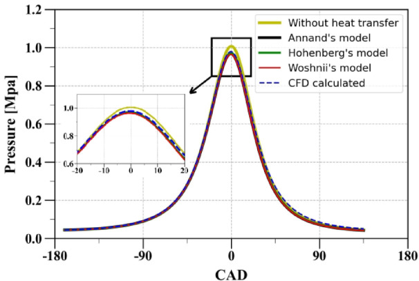
Comparison of in-cylinder motoring pressure obtained using various heat transfer models.

Gas exchange process

The gas exchange process involves the study of the intake and exhaust processes of a four-stroke internal combustion (IC) engine. The main objective of the gas exchange process is to calculate the mass trapped in the engine cylinder from the exhaust valve opening (EVO) CAD to the intake valve closing (IVC) CAD and the pressure and temperature of the in-cylinder charge during this period.

Thermodynamic modeling

During the gas exchange phase, the control volume of the engine cylinder involves mass, heat, and work interaction from its boundary. Therefore, to calculate in-cylinder pressure, temperature, and mass during the gas exchange phase, the first law of thermodynamics for an open system, the ideal gas equation, and the mass flow rate equation of compressible fluid are used.

The following assumptions were made for developing governing equations during the gas exchange phase:

• I.During the exhaust stroke, in-cylinder gases are a mixture of different ideal gases formed as products of fuel combustion.
• II.During the intake stroke, in-cylinder gases are a mixture of air, fuel and recycled burned exhaust gases that remain after the end of the exhaust stroke.
• III.No spatial variation of in-cylinder thermodynamic properties.

The first law of thermodynamics for an open system in differential form as a function of crank angle () is given in Eq. (50).

50

Where is the total internal energy, is the net heat transfer from the system boundary, is the work done by the gas, and are specific enthalpy and mass flow from the intake manifold, and are specific enthalpy and mass flow from the exhaust manifold.

Assuming no changes in kinetic and potential energy of the system, Eq. (50) is written to calculate in-cylinder pressure as a function of crank angle and presented in Eq. (51)²⁵ :

51

Where is the in-cylinder pressure, is the cylinder volume, is the specific heat ratio of in-cylinder gas mixture, is the characteristic gas constant of in-cylinder gas mixture, and are temperature of gas mixture flowing through intake and exhaust manifold, respectively.

In-cylinder temperature is calculated using ideal gas equation:

52

The in-cylinder mixture properties, and are calculated as explained in Sect. 3.1 (thermodynamic property calculation). Instantaneous volume can be calculated by geometrical parameters of the engine and compression ratio and given by¹⁴:

Mass flow rate calculation

Mass flow rates through the intake and exhaust manifolds, the third term on the right-hand side of Eq. (51) are calculated using isentropic compressible flow equations²⁵.

53

Where is the flow area, subscript u denotes upstream, R is the characteristic gas constant of the in-cylinder gas mixture, and F is the expansion factor that depends on flow condition (choked or non-chocked flow).

For non-chocked flow:

54

For chocked flow:

55

Coefficient of discharge

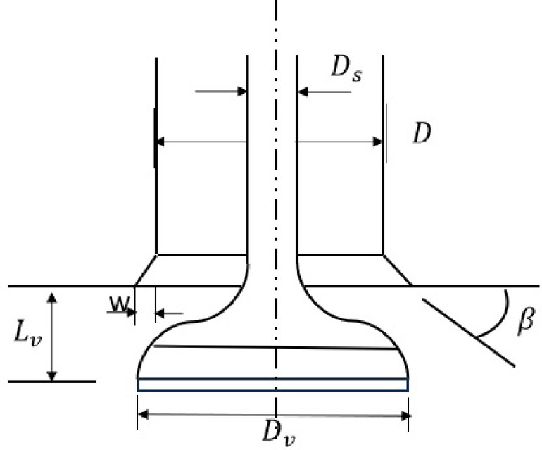
Kastner et al.²⁶ investigated the parameters of valve geometry (Fig. 5) that affect the flow area through the valves. As the intake and exhaust valves open and close, the flow area and coefficient of discharge change. Kastner developed a correlation (mentioned below) for the coefficient of discharge as a function of ratio of the valve lift () and inner seat diameter of poppet (D) valve.

56

Fig. 5.

Parameters defining poppet valve geometry.

Flow area

The flow area is calculated as the function of poppet valve geometry and valve lift. Based on the instantaneous valve lift value, the flow area calculation is divided into three stages (Fig. 6) and calculated as follows¹⁴:

Fig. 6.

Three stages of flow area.

For the first stage, when the valve lift has low value, the flow area corresponds to a frustum of a cone. The flow area is calculated by the distance along the conical face of the valve and the seat.

In this stage:

57

Where is the seat width, is the valve seat angle, and is the valve head diameter.

In the second stage the flow area is between the seat and the nearest edge of the valve.

58

Where is the port diameter, is the stem diameter, and is the mean seat diameter ().

In the third stage the flow area is the area of the port minus the area of the valve stem.

59

Model validation

In-cylinder pressure and mass obtained from the results of 0D model are validated with the results of CFD model and presented in Fig. 7. In addition, the normalized in-cylinder properties were also calculated to establish a comparison with the data from available literature and presented in Fig. 8.

Fig. 7.

Comparison of (a) cylinder pressure (b) mass of gases inside the cylinder.

Fig. 8.

Variation of various normalized properties with crank angle during gas exchange period obtained by (a) by 0D model (b) Heywood¹⁴.

Compression and expansion strokes

During compression and expansion strokes, the in-cylinder pressure and temperature vary with respect to cylinder volume (or CAD). The variation can be computed by developing governing equations by considering the cylinder as a closed system and by applying first law of thermodynamics and ideal gas equation. The following assumptions were made while developing the governing equations:

• I.No mass transfer happens from the engine cylinder region to the crevice region.
• II.At any particular instant of time, pressure and temperature inside the cylinder region are homogeneous throughout the cylinder volume.
• III.During the compression stroke, in-cylinder gases are a mixture of trapped exhaust gases and fresh charge entered during the intake stroke.
• IV.During the expansion stroke, in-cylinder gases are a mixture of different burned ideal gases.

The first law of thermodynamics (for a closed system) is given by:

60

Similar to the procedures followed while developing governing equations for gas exchange process, the Eq. (60) can also be written in terms of pressure and volume variables.

61

Temperature is calculated by ideal gas equation:

62

The in-cylinder mixture properties are calculated using thermodynamic property calculations as explained in Sect. 3.1.

Combustion process

The combustion process releases the chemical energy stored in the fuel, resulting in an elevation of both in-cylinder temperature and pressure. Subsequently, the combustion products (burned gases) undergo expansion, transferring their energy to the piston. The thermodynamics-based modeling of the combustion process can be categorized into two groups: single-zone models and multi-zone models, and they are explained below.

Single zone model

Yildız and Çeper²⁷ employed a single zone combustion model where the combustion chamber is treated as a single control volume, and the analysis is conducted using the first law of thermodynamics and the ideal gas law. The governing equations for in-cylinder temperature and pressure are given in Eqs. (63) and (64).

63

64

Where , , and represent the in-cylinder pressure, temperature, and volume, respectively, and is the specific heat ratio of the in-cylinder gas mixture. The limitation of the single-zone combustion model is that it provides only the mean in-cylinder temperature. When performing emission analysis using chemical kinetics (as explained in Sect. 3.6), this limitation can lead to significant errors because reaction rates strongly depend on temperature, and a large temperature gradient exists inside the cylinder during the combustion process. Hence, a multi-zone model becomes necessary for the precise calculation of emission formation.

Multi-zone model

In a multi-zone combustion model, the combustion chamber is partitioned into multiple zones, and separate analyses are conducted for each zone. The number of zones into which the cylinder is divided affects both the accuracy and computational time. Verhelst and Sheppard²¹ employed a two-zone combustion model, where the cylinder volume was divided into two zones namely the burned zone and the unburned zone, separated by a flame front. Figure 9 illustrates the schematic of a conventional two-zone thermodynamics-based model. The assumptions involved in the development of two-zone combustion model are as follows²⁸:

Fig. 9.

Schematic diagram of two-zone combustion model.

• I.The unburned zone contains a homogeneous fresh fuel-air mixture and some fraction of exhaust gases from the previous cycle.
• II.The combustion products formed during the combustion process are assumed to remain only in the burned zone.
• III.Pressure is uniform in both zones and varies only with time.
• IV.Temperature and other thermodynamic properties differ for both zones.
• V.No heat transfer between burned and unburned zones.

Considering the above assumptions, governing equations were derived to compute burned zone temperature, unburned zone temperature, and in-cylinder pressure by applying the first law of thermodynamics and ideal gas equation separately for both zones.

The temperature of gases in the unburned zone is calculated as a function of the crank angle and presented in Eq. (65)²⁸.

65

Where is the unburned gas temperature, is the mass of gases in the unburned zone, is the specific heat at constant pressure of in-cylinder gas mixture in the unburned zone, is the volume of gases in the unburned zone, is the in-cylinder pressure, and is the heat transfer through the wall of the unburned zone.

The temperature of gases in the burned zone is calculated as a function of the crank angle and presented in Eq. (66)²⁸.

66

Where is the burned gas temperature, is the mass of gases in the unburned zone, is the characteristic gas constant of in-cylinder gas mixture in the unburned zone, is the specific heat at constant pressure of in-cylinder gas mixture in the burned zone, is the volume of gases in the burned zone, is in-cylinder pressure, is cylinder volume, is heat transfer through the wall of the burned zone, is mass burn rate, is the leakage of unburned gas from the cylinder to crankcase, and is the leakage of burned gas from cylinder to crankcase.

In-cylinder pressure is calculated as a function of the crank angle and presented in Eq. (67)²⁸.

67

To solve Eqs. (65), (66), and (67), the values of , , ,,, are required in prior and are calculated as explained in Sect. 3.1. The terms , are neglected because of their minimal influence. The model requires the term as input and can be provided by calculating mass fraction burned . The methods available for computing mass fraction burned are explained below.

Modeling of mass fraction burned

During the combustion period, the variation of in-cylinder pressure and temperature w.r.t to CAD in burned and unburned zones mainly depends on the rate of energy released by burning of fuel. Therefore, to accurately model the combustion process it is important to predict the rate of fuel burned accurately. Two approaches are discussed below to predict the mass fraction burned:

Co-sine function

In this approach, the variation of mass fraction burned w.r.t. crank angle is computed using the Eq. (68)²⁹.

68

Where is the instantaneous crank angle, is the value of crank angle where combustion starts, is the total combustion duration. The limitation of this function is there is no adjustable parameter to fit the mass fraction burned curve close to the experimental curve.

Single Wiebe function

The limitations of the co-sine function can be overcome by the Wiebe function³⁰ presented in Eq. (69), which consists of two adjustable model parameters (, ).

69

Where is called efficiency parameter tuning its value controls the combustion duration, is the form factor. The values of and should be tuned to obtain the computed mass fraction burned curve close to the experimental curve.

To calculate the mass fraction burned curve from the models mentioned above, the parameter combustion duration () is required. Two approaches are discussed below to calculate the combustion duration: (a) Correlation based on engine speed and equivalence ratio, (b) By analysis of heat release rate.

(a) Calculation of combustion duration based on correlation - To calculate combustion duration, a correlation was developed by Campbell³¹ based on experimental data reported by Taylor³², which takes engine speed and equivalence ratio as inputs and is presented in Eq. (70).

70

(b) By analysis of heat release rate - The combustion duration can also be determined by analyzing the heat release rate from the experimentally obtained in-cylinder pressure. Prior to the initiation of the combustion process, the in-cylinder heat release rate results from the heat transfer between the cylinder wall and in-cylinder gases. During the combustion process, the in-cylinder heat release rate is attributed not only to the heat transfer between the cylinder wall and in-cylinder gases but also to the heat released with the combustion of the fuel. The chemical heat released () by the fuel as a function of crank angle, assuming no crevice effect, is provided in Eq. (71)³³:

71

Where the constant value of the specific heat ratio is assumed. , are the in-cylinder pressure and volume. is the heat transfer through the cylinder wall calculated using Hohenberg’s heat transfer model.

Figure 10 presents the cumulative heat release curve for operating conditions mentioned in Table 1, represents the maximum heat released by the fuel, where is the mass of the fuel per cycle and is the lower heating value of the fuel. denotes the net heat released, and when heat transfer from the wall is added to the net heat released, it gives the total chemical energy released (). The point at which the chemical heat release rate deviates signifies the start of combustion. It is challenging to precisely determine the end of combustion from the heat release rate curve because, at the conclusion of combustion, the rate of heat released is nearly equivalent to the heat transfer from the cylinder wall. In SI engines, the crank angle corresponding to 90% or 95% of the total heat released from the fuel is typically considered as the end of combustion³³. In this study, the crank angle corresponding to 90% heat release is adopted as the end of combustion.

Fig. 10.

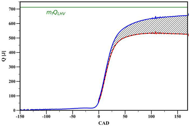
Cumulative heat release.

Model validation for fraction of mass burned

From the analysis of heat release rate for the operating conditions mentioned in Table 1, the start of combustion and total combustion duration are found to be −16 CAD and 60 CAD, respectively. Whereas the combustion duration is found to be 59.3 CAD when calculated using correlation model (presented in Eq. (70)). Figure 11 shows the performance of the cosine and single Wiebe function model (with = 4.448 and= 1.762) and its comparison with experiment mass fraction burn curve. The values of and of the single Wiebe function are found by minimizing the mean squared error (MSE) between predicted and experimental mass fraction burned.

Fig. 11.

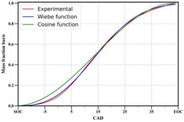
Comparison of mass fraction burned predicted by the cosine function and Wiebe function with experimental result.

Combustion model validation

Figure 12 presents the comparison of the in-cylinder pressure and mean temperature during compression, combustion, and expansion strokes for operating conditions mentioned in Table 1 obtained from 0D models and CFD model. The mean cylinder temperature is calculated by:

Fig. 12.

Comparison of (a) in-cylinder, (b) mean cylinder temperature.

Emission modeling

In internal combustion engines, during the combustion of fuel, some harmful pollutant species are also formed. These pollutants leave the engine cylinder during the exhaust stroke and enter into the atmosphere, causing harmful health and environmental effects. The major exhaust emissions are unburned hydrocarbons (HC), oxides of carbon (CO and CO₂), oxides of nitrogen (NO and NO₂), and particulate matter. The total amount of pollutant emission mainly depends on the type of fuel, equivalence ratio, in-cylinder temperature, and other engine operating parameters. For SI engines, unburned hydrocarbons, oxides of carbon and oxides of nitrogen (also called NO_X) are the main components of pollutants. This section presents chemical kinetics-based thermodynamics-based modeling and validation of nitrogen oxide (NO), and carbon monoxide (CO) emissions.

Modeling of nitrogen oxide emissions

In general, oxides of nitrogen (NOx) formation in IC engines can primarily occur through four routes: the thermal route, prompt route, N₂O route, and fuel route. However, the thermal route is the major contributor, accounting for more than 90% of NOx formation. The extended Zeldovich mechanism described by the following three equations accounts for the formation of NOx through the thermal route and is widely used³⁴:

72

73

74

It is assumed that O, O₂, N₂, OH and H are at equilibrium, and due to their low concentration, atomic nitrogen (N) is assumed to be in a steady state.

75

Considering these assumptions, the rate of change of concentration of nitrogen oxide is written as³⁴:

76

Where V is the cylinder volume, n_NO is the moles of nitrogen oxide, [] represents the species concentration, and []_e represents the species concentration at equilibrium. R₁, R₂, R₃ are the equilibrium reaction rates for Eqs. (72, 73 and 74), respectively, and they are computed as follows:

	Where
	Where
	Where

Where and represent the reaction rate constants in cm³/mol-s for the i^th reaction, corresponding to the forward and backward reactions, respectively.

Modeling of carbon monoxide emission

When the combustion process is initiated (either by a spark or compression ignition), the hydrocarbon fuel starts breaking down and forms many intermediate species prior to the formation of stable species like CO₂ and H₂O. CO is such an intermediate species and forms a path for the formation of CO₂ during the oxidation of hydrocarbon fuel. Insufficient oxygen availability, reducing temperatures (due to downward piston motion), and slow combustion generally result in high engine-out CO species. The following two reactions are crucial to compute the kinetically controlled formation and decomposition of carbon monoxide³⁴:

77

78

Assuming that , , are in the thermal equilibrium, the rate of change of concentration of carbon monoxide is written as³⁴:

79

Where is the moles of carbon monoxide, R₄ and R₅ are the equilibrium reaction rates for Eqs. (77) and (78), respectively and they are computed as follows:

	where
	Where

Model validation

Figure 13 presents the performance of the thermodynamics-based emission models used for nitrogen oxide and carbon monoxide emissions and its comparison with the CFD model for operating conditions mentioned in Table 1.

Fig. 13.

Comparison between 0D model and CFD model for (a) NO and (b) CO emissions.

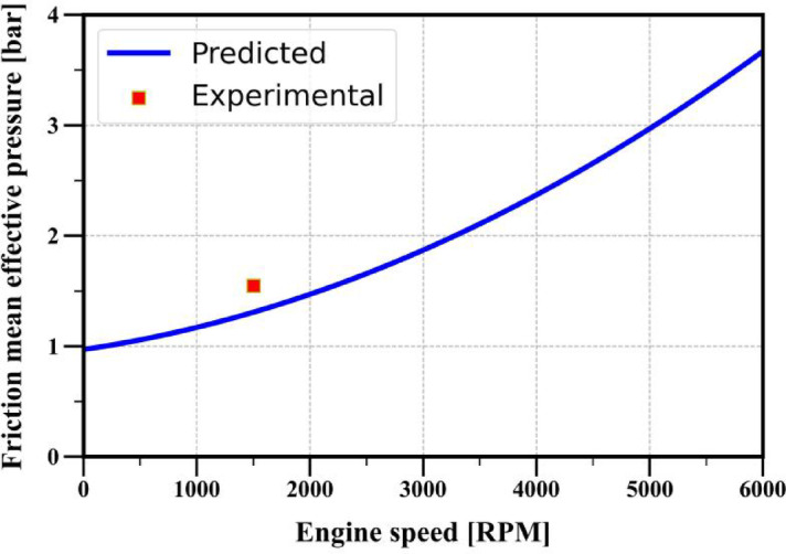
Friction modeling

Friction within an internal combustion engine is a critical factor that significantly impacts its overall performance and efficiency. The power available at the crankshaft (break power) is significantly lower than the gross indicated power (developed during compression and expansion strokes), and the difference between break power and gross indicated power is called friction power.

A correlation was developed to predict the friction mean effective pressure (FMEP) (ratio of friction work and displacement work)¹⁴ based on experimental data from various four-stroke SI engines. The correlation predicts the friction mean effective pressure based on engine speed and is given in the Eq. (80):

80

Where N is the engine speed in revolutions per minute (RPM). Hence, in the context of friction modeling, Eq. (80) is utilized, taking engine speed as an input to calculate the friction mean effective pressure.

Model validation

Figure 14 presents the validation of the friction model. FMEP predicted by the correlation mentioned (Eq. (80)) is validated by experimentally obtained FMEP for operating conditions mentioned in Table 1. The procedure for calculation of experimental friction mean effective pressure is given below:

81

Fig. 14.

Comparison between experimentally obtained and correlation model predicted friction mean effective pressure.

Where gross indicated work is the work delivered to the piston over the compression and expansion strokes calculated by over the compression and expansion strokes.

82

Where break work is calculated by where is the break torque measured from the experiment and is the number of crankshaft revolutions during one power cycle (1 for two-stroke and 2 for four-stroke engines).

Full cycle simulation

In the previous section, various sub-models to analyze individual in-cylinder processes within a spark ignition engine were discussed. These sub-models offer valuable insights into specific aspects of engine operations under consideration. However, a full-cycle simulation can provide a more accurate representation of the engine performance as it enables us to account for interactions and dependencies between different in-cylinder processes. Since full-cycle simulation is a combination of in-cylinder processes presented in Sect. 3, a flow chart is shown in Fig. 15, which connects all the in-cylinder phenomena in order to complete an engine cycle simulation.

Fig. 15.

Flow chart for full engine cycle simulation.

Results and discussion

The performance of a full-cycle simulation by integrating various in-cylinder phenomena is presented in Fig. 16. The engine specifications and operating conditions used for full-cycle simulation are provided in Table 1. The performance of the phenomenological model is validated by comparing its performance with the CFD model. As mentioned earlier, the performance of the phenomenological model depends on the accuracy of the sub-model employed for individual in-cylinder phenomena. Therefore, while performing a full cycle simulation, a two-zone model is used for combustion modeling, a single Wiebe function is employed to calculate the burned mass fraction, Hohenberg correlation is utilized to calculate the in-cylinder heat transfer and in-cylinder mixture properties are evaluated based on mixture composition.

Fig. 16.

Comparison of (a) in-cylinder pressure (b) in-cylinder temperature obtained from full cycle simulation for methane fuel, compression ratio 10.1:1, and load 10 N-m.

Full-cycle simulations are also conducted to assess the model’s capability to accurately depict the impact of variations in operating conditions. In this context, a thermodynamic simulation is executed with the operating parameters identical to those specified in Table 1, with the exception of using gasoline as the fuel, setting the compression ratio to 8.5:1, maintaining an equivalence ratio of 1, and at 12 N-m loading conditions. The in-cylinder pressure and NOx emission are predicted using the developed code and compared with the experimentally obtained data (Fig. 17) reported by Gupta and Mittal³⁵. Figure 17 shows that the 0D model is able to predict the results with good accuracy even under different operating conditions.

Fig. 17.

Comparison of (a) in-cylinder pressure (b) in-cylinder temperature obtained from full cycle simulation for gasoline fuel, compression ratio 8.5:1, and load 12 N-m.

Summary and conclusions

In this paper, various in-cylinder phenomena – including gas exchange, compression, expansion, mixture properties calculation, heat transfer, fuel burn rate, combustion, exhaust emissions, and frictional losses – were modeled using zero-dimensional (0D) thermodynamics-based models. The gas exchange process was modeled by applying the mass conservation law and the first law of thermodynamics for an open system, whereas compression and expansion processes were modeled using the first law of thermodynamics for a closed system. Mixture properties were calculated using established correlations and equilibrium-based models, with validation results indicating that equilibrium-based models provided higher accuracy across a wide range of thermodynamic states. For in-cylinder heat transfer calculations, various empirical correlations were employed. The fraction of fuel burned rate was calculated using a cosine function and a single Wiebe function, with the Wiebe function demonstrating better agreement with experimental data when its parameters were appropriately tuned. Combustion was modeled using both single-zone and two-zone approaches. The burned and unburned zone temperatures obtained from the two-zone combustion model were then utilized in chemical kinetics-based emission modeling, and its performance was compared with results from computational fluid dynamics (CFD)-based models. Frictional losses were estimated using an established correlation dependent on engine speed. Finally, full engine cycle simulations were performed by integrating all sub-models under various operating conditions. The results from these simulations were validated against both CFD-based model results and experimental data, demonstrating the effectiveness of the proposed modeling approach.

Author contributions

M.M. Conceptualization and Methodology. C.K.C. Software development. C.K.C. and P.S.V. Validation, Investigation and Formal analysis. M.M. Project administration and Supervision. C.K.C. and P.S.V. Wrote the main manuscript text. MM review and editing.

Data availability

The datasets used and/or analysed during the current study available from the corresponding author on reasonable request.

Declarations

Competing interests

The authors declare no competing interests.

References

- 1.Marinoni, A. et al. 0D/1D thermo-fluid dynamic modeling tools for the simulation of driving cycles and the optimization of IC engine performances and emissions. Appl. Sci.11 (17), 8125 (2021). [Google Scholar]
- 2.Onorati, A. & Montenegro, G. 1D and multi-D Modeling Techniques for IC Engine Simulation (SAE International, 2020).
- 3.Saied, O. M. & Abdelwahab, M. 1D hydrogen engine modeling to investigate air-fuel ratio, spark timing, and water injection effects on performance and emissions. Sci. Rep.15 (1), 1–19. 10.1038/s41598-025-00952-0 (2025). [DOI] [PMC free article] [PubMed] [Google Scholar]
- 4.Shaik, F. et al. Predictive modeling and optimization of SI engine performance and emissions with GEM blends using ANN and RSM. Sci. Rep.15 (1), 1–23. 10.1038/s41598-025-88486-3 (2025). [DOI] [PMC free article] [PubMed] [Google Scholar]
- 5.Ma, Y. et al. Combustion and emission characteristics of ammonia-diesel marine high pressure direct injection low-speed dual-fuel engine. Sci. Rep.15 (1), 1–12. 10.1038/s41598-025-04997-z (2025). [DOI] [PMC free article] [PubMed] [Google Scholar]
- 6.Fogla, N., Bybee, M., Mirzaeian, M., Millo, F. & Wahiduzzaman, S. Development of a K-k-ɛ phenomenological model to predict in-cylinder turbulence. SAE. Int. J. Engines. 10 (2), 562–575. 10.4271/2017-01-0542 (2017). [Google Scholar]
- 7.Sadafale, S. S., Mittal, M. & Inaba, K. Phenomenological modeling and experiments to investigate the combined effects of high pressure and multiple injection strategies with EGR on combustion and emission characteristics of a CRDI diesel engine. SAE Tech. Pap.10.4271/2019-01-0056 (2019).
- 8.George, S. M., Gupta, S. K. & Mittal, M. Phenomenological modeling to study the combustion emission characteristics of a spark-ignition engine. 12th Asia-Pacific Conference on Combustion, ASPACC 2019. (2019).
- 9.Gupta, S. K. & Mittal, M. Effect of compression ratio on the performance and emission characteristics, and cycle-to-cycle combustion variations of a spark-ignition engine fueled with bio-methane surrogate. Appl. Therm. Eng.148, 1440–1453. 10.1016/j.applthermaleng.2018.11.057 (2019). [Google Scholar]
- 10.Kurien, C., Varma, P. S. & Mittal, M. Effect of ammonia energy fractions on combustion stability and engine characteristics of gaseous (ammonia/methane) fuelled spark ignition engine. Int. J. Hydrogen Energy. 48 (4), 1391–1400. 10.1016/j.ijhydene.2022.10.032 (2023). [Google Scholar]
- 11.Bundele, H., Kurien, C., Varma, P. S. & Mittal, M. Experimental and computational study on the enhancement of engine characteristics by hydrogen enrichment in a biogas fuelled spark ignition engine. Int. J. Hydrog. Energy. 47 (71), 30671–30686. 10.1016/j.ijhydene.2022.07.029 (2022). [Google Scholar]
- 12.Sandeep Varma, P. & Mittal, M. Investigations with bowl-in-piston (CI type) and flat-piston (SI type) geometries to study the engine characteristics of a CI engine retrofitted for SI operation with CNG fuel. Energy Conv. Manag.301 118083. 10.1016/j.enconman.2024.118083 (2024).
- 13.Gupta, S. K. & Mittal, M. A CFD study on the effect of compression ratio on combustion characteristics and emissions in a spark-ignition engine. Progress Comput. Fluid Dynamics. 20 (5), 299–306. 10.1504/PCFD.2020.109903 (2020). [Google Scholar]
- 14.Heywood, J. B. Internal Combustion Engine Fundamentals (McGraw-Hill, 1988).
- 15.JANAF Thmnochemical Tables. 2d ad., NSRDS-NB537, U.S. National Bureau of Standards. (1971).
- 16.Olikara, C. & Borman, G. L. A computer program for calculating properties of equilibrium combustion products with some applications to I.C. Engines. SAE Tech. Pap.10.4271/750468 (1975).
- 17.Morley, C. GasEQ: A chemical equilibrium program for windows. 27http://www.gaseq.co.uk/ (2007).
- 18.Gatowski, J. A. et al. Heat release analysis of engine pressure data. SAE Tech. Papers. 93, 961–977. 10.4271/841359 (1984). [Google Scholar]
- 19.Brunt, M. F. J., Rai, H. & Emtage, A. L. The calculation of heat release energy from engine cylinder pressure data. SAE Tech. Papers. 724. 10.4271/981052 (1998).
- 20.Hohenberg, G. & Killman, I. Basic findings from measurement of the combustion process, XIX Fisita Congress, Melbourne, Australia, paper 82126. (1982).
- 21.Kayadelen, H. K. Effect of natural gas components on its flame temperature, equilibrium combustion products and thermodynamic properties. J. Nat. Gas Sci. Eng.45, 456–473. 10.1016/j.jngse.2017.05.023 (2017). [Google Scholar]
- 22.Annand, W. J. D. Heat transfer in the cylinders of reciprocating internal combustion engines. Proc. Inst. Mech. Eng.177 (36), 973–990. (1963).
- 23.Woschni, G. A universally applicable equation for the instantaneous heat transfer coefficient in the internal combustion engine. SAE Tech. Papers. 10.4271/670931 (1967). [Google Scholar]
- 24.Hohenberg, G. F. Advanced approaches for heat transfer calculations. SAE Tech. Pap. 2788–2806. 10.4271/790825 (1979).
- 25.Sherman, R. H. & Blumberg, P. N. The influence of induction and exhaust processes on emissions and fuel consumption in the spark ignited engine. SAE Tech. Papers. 10.4271/770880 (1977). [Google Scholar]
- 26.Kastner, L. G., Williams, T. J. & White, J. B. Poppet inlet valve characteristics and their influence on the induction process. Proc. Inst. Mech. Eng.178, 955. (1963).
- 27.Yıldız, M. & Albayrak Çeper, B. Zero-dimensional single zone engine modeling of an SI engine fuelled with methane and methane-hydrogen blend using single and double Wiebe function: A comparative study. Int. J. Hydrog. Energy. 42 (40), 25756–25765. 10.1016/j.ijhydene.2017.07.016 (2017). [Google Scholar]
- 28.Verhelst, S. & Sheppard, C. G. W. Multi-zone thermodynamic modelling of spark-ignition engine combustion - An overview. Energy. Conv. Manag.50 (5), 1326–1335. 10.1016/j.enconman.2009.01.002 (2009). [Google Scholar]
- 29.Blumberg, P. & Kummer, J. T. Prediction of NO formation in Spark-Ignited Engines—An analysis of methods of control. Combust. Sci. Technol.4 (1), 73–95. 10.1080/00102207108952474 (1971). [Google Scholar]
- 30.Heywood, J. Engine combustion modeling-an overview. Combustion modeling in reciprocating engines. 1–35. (1980).
- 31.Campbell, A. S. Thermodynamic Analysis of Combustion Engines (Wiley, 1979).
- 32.Taylor, C. F. The Internal Combustion Engine in Theory and PracticeII, Chap. 1. (MIT Press, 1968).
- 33.Liu, J. & Dumitrescu, C. E. Single and double Wiebe function combustion model for a heavy-duty diesel engine retrofitted to natural-gas spark-ignition. Appl. Energy. 248 (April), 95–103. 10.1016/j.apenergy.2019.04.098 (2019). [Google Scholar]
- 34.Arsie, I., Pianese, C. & Rizzo, G. Models for the prediction of performance and emissions in a spark ignition engine - A sequentially structured approach. SAE Tech. Papers. 724. 10.4271/980779 (1998).
- 35.Gupta, S. K. & Mittal, M. Effect of compression ratio on the performance and emission characteristics, and Cycle-to-Cycle combustion variations of a Spark-Ignition engine fueled with Bio-methane surrogate. Appl. Therm. Eng.148, 1440–1453. 10.1016/j.applthermaleng.2018.11.057 (2019). [Google Scholar]
Associated Data
This section collects any data citations, data availability statements, or supplementary materials included in this article.
Data Availability Statement