Integrating double techniques of statistical downscaling and bias correction to reduce bias in projections trends of future climate datasets

Abstract

Climate change is one of the most significant challenges of the 21st century, particularly its impact on surface water availability in arid and hyper-arid regions within the Euphrates River Basin. This study aims to analyze the impacts of climate change using five global climate models (GCMs) within the Coupled Model Intercomparison Project Phase 6 (CMIP6, IPCC 2021). Model outputs were statistically downscaled using Statistical Downscaling Model (SDSM 6.1) under three greenhouse gas emission scenarios, and bias correction was performed using Climate Model Data for Hydrologic Modeling (CMhyd 1.02). Performance evaluation was based on data from meteorological stations distributed across five climatic zones within the basin, covering the period from 1982 to 2023. The study results showed that the uncertainty-related biases in CMIP6 models limit the accuracy of climate projections in the basin. Using individual GCM models instead of relying solely on linear trends can reduce bias and uncertainty in estimating climate variables across different regions. Although the SDSM model provides a good fit with GCM outputs, the variability in spatial patterns and emission scenarios is reflected in the limited accuracy of some climate indices. Applying bias correction using the linear scaling method has been shown to improve the accuracy of statistical modeling. Projections indicate that rising temperatures due to increased greenhouse gas emissions may decrease rainfall in arid regions while increasing in humid regions. These results contribute to a better understanding of climate change’s impacts on water resources in river basins and provide a scientific basis for developing effective adaptation strategies and future planning.

Supplementary Information

The online version contains supplementary material available at 10.1038/s41598-025-15483-x.

Introduction

Global climate models (GCMs) driving the sixth phase of the coupled model intercomparison project (CMIP6) are used to model weather phenomena associated with global warming and to predict atmospheric circulation patterns on a global scale. However, questions remain about the consistency of the physical frameworks and models used, particularly regarding their ability to reproduce annual and decadal climate variability^1,2 accurately. Significant declines in accuracy are observed when GCMs are used over longer timescales^3,4. Employing bias correction and downscaling techniques is an important step toward improving the accuracy of GCM outputs, especially given the challenges associated with their low accuracy at local and regional scales^5–7. Combining these two techniques helps address model shortcomings, enhancing the reliability of climate projections at finer temporal and spatial output scales^8,9.

Statistics projection becomes more effective and relevant to climate change research when downscaling techniques are applied, translating global weather systems’ effects into climate indicators at local levels¹⁰. Downscaling is one of the most effective tools for improving the approximate spatial resolution of global climate model outputs, transforming their data into high-resolution data, enabling a more accurate representation of regional and local climate changes^11–13.

Downscaling techniques are generally classified into two main types: statistical and dynamical methods. Statistical methods are based on the outputs of GCMs, while dynamical methods are based on regional climate models (RCMs)¹⁴. In statistical downscaling, various deterministic or stochastic methods are used to extract accurate local climate information from global climate models’ large-scale, generalized data. These methods are based on statistical or physical relationships between climate phenomena at the regional and global scales¹⁵. These techniques rely on what are known as cross-scale relationships, where regional variables such as temperature and precipitation are directly linked to larger-scale atmospheric circulation patterns. As a result, climate projections produced by these methods are also cross-scale, enhancing their ability to represent local climate conditions with greater accuracy within specific time and spatial frameworks^16–18.

Statistical downscaling techniques determine climate patterns by supporting various methods, such as multiple regression approaches, weather generators, and classification procedures that apply to multiple temporal and spatial scales. These methods analyze relationships between significant climate variables and local climate indices, contributing to a better understanding of regional climate systems¹⁹. Statistical downscaling is essentially based on three underlying assumptions: (1) This technique assumes that the selected predictor variables accurately represent the outputs of GCMs and can capture relevant climate characteristics. (2) It is assumed that the validated empirical relationships, established over historical observation periods, remain valid and applicable under changing future climate conditions. (3) It is assumed that GCMs are not subject to the same statistical rules or mechanisms used in other climate models, allowing statistical downscaling techniques without affecting the structural consistency of the original model^20–22. Statistical downscaling techniques do not always guarantee an accurate representation of the complex relationship between the climate system as simulated by GCMs, emissions scenarios, and local climate outcomes^23,24.

The Statistical Downscaling Model (SDSM) is one of the most popular and widely used tools in climate research due to its ability to reproduce observed climate variability²⁵ accurately. The program relies on hybrid models that combine regression-based approaches with components from stochastic weather generators, enabling it to efficiently simulate the correlations between local and global climate variables^26,27. This methodology improves downscaling accuracy at both the local and macroscales. The downscaling process includes the uncertainties of spatial resolution of GCMs, emissions scenarios, and the assumptions of downscaling technique like empirical connections linking predictors and predictions^28,29.

To achieve more accurate results in downscaling, it is essential to reduce biases in output data, which often arise from the inaccurate representation of atmospheric physics across various climate zone³⁰. This procedure significantly reduces uncertainty and bias, enhancing the reliability and utility of downscaled climate data in a wide range of applications³¹. Numerous studies^32–35 have shown that applying bias correction effectively reduces the uncertainty associated with downscaling results using GCMs, thereby improving the quality of the climate data. Post-processing and adjusting the downscaled output data to match reference data or actual climate observations are crucial. Different bias correction methods rely on the assumption of constancy of the statistical relationship used, requiring future climate data to undergo the same correction process as historical climate data to ensure consistency and continuity^36–38.

The linear scaling bias correction method is effective for adjusting the frequency of weather data³⁹. Its simplicity and ease of application make it a popular choice, especially in situations requiring rapid adjustments to climate model output simulations. Climate Model Data for Hydrologic Modeling (CMhyd) program contributes to enhancing the accuracy and consistency of hydrological modeling by correcting the bias in climate model data used in this context, whether produced by regional or global climate models^40,41. Despite the importance of these treatments in improving the representation of climate conditions, studies have not yet adequately addressed the uncertainty associated with climate change projections produced by GCMs, particularly about their varying impacts on different climate zones within the Euphrates River study area.

The Intergovernmental Panel on Climate Changes (IPCC, 2021, AR6) provided the future weather dataset for the study area projections under three scenarios of Shared Socioeconomic Pathways (SSPs). These three SSP scenarios, low intensity (SSP1–2.6), medium intensity (SSP2–4.5), and high intensity (SSP5–8.5), provide a representative range of possible impacts of climate change in the future.

The main goals of this research are four main points: (1) to assess the uncertainty associated with GCMs to understand and analyze CMIP6 climate datasets. (2) to evaluate the efficiency of SDSM 6.1 in producing downscaled temperature and precipitation datasets with local-level accuracy; (3) to apply a bias correction model CMhyd 1.02 to the downscaled climate projection data to improve their quality and reduce biases; and (4) to generate future projections of temperature and precipitation trends under three SSP scenarios.

Methodology and resources

Study area

One of the longest rivers in West Asia is the Euphrates River Basin (ERB), originating in Turkey near the Armenian Highlands⁴². The study reach of the basin extends approximately 1,002 km from the Birecik dam to the Haditha dam reservoir in Turkey. Figure 1 shows the ERB’s location generated using Geographic Information Systems (Arc GIS 10.5); the climate of the ERB is influenced by its topography, geographic location, and prevailing weather systems. According to⁴³, the region’s climate ranges from moist to dry-subhumid in the east and north and from semi-arid to hyper-arid in the south. The lowlands’ average annual precipitation of around 90 mm shows a dry environment with little precipitation. Around 910 mm of precipitation falls in the upper reaches close to the mountains yearly. Rivers rely on this precipitation as their primary water supply, which keeps them flowing and guarantees water downstream⁴⁴. Average annual temperatures in the region range from 17 to 29 C, and summers are usually hot, especially in the lower elevations.

Fig. 1.

A location and topography of study area within Euphrates River Basin represented by (Arc GIS 10.5).

GCMs projections with future scenarios

Global climate data is mainly derived from GCMs created under CMIP6 by the World Climate Research Program. Following the IPCC 2021 release of its sixth assessment report (AR6), CMIP6 is essential for understanding current climate conditions and predicting future events as greenhouse gas concentrations increase. Critical meteorological variables are provided by GCMs, which also interpret the complexities of the atmosphere. These complex numerical representations of the climate system on Earth enhance the IPCC and other climate assessments. Using historical runs from six GCMs with varied labels, CMIP6 presents “Tier 1” experiments. (r1i1p1f1) extent from 1850. The several CMIP6 models are described in detail in (Table 1), along with their resolutions and sources. The diversity of model properties, including resolution, parameterizations, ensembles, and initialization, allows for a detailed investigation of the uncertainties in climate projections from the Earth System Grid Federation archives. Five climatic zones, humid, dry sub-humid, semi-arid, arid, and hyper-arid, have been identified for the chosen research region due to its varied climate. The general climate and topography of the area distinguish these zones. Geographic Information Systems (Arc GIS 10.5) were used to draw the map of the research region’s climatic zones (Fig. 2).

Table 1.

CMIP6 climate model selection within study area.

(GCMs)	Country	Horizontal resolution		Normal resolution	Variant label
		longitude	latitude
BCC-CSM2-MR	China	1.125◦	1.125◦	100 Km	r1i1p1f1
CanESM5	Canada	2.81◦	2.81◦	500 Km	r1i1p1f1
CNRM-CM6-1	France	1.4◦	1.4◦	250 Km	r1i1p1f2
HadGEM3-GC31-LL	UK	1.88◦	1.25◦	250 Km	r1i1p1f3
MRI-ESM2-0	Japan	1.125◦	1.125◦	125 Km	r2i1p1f1

Fig. 2.

Detailed climatic zones classification of the study areas within the Euphrates River Basin based on the approved climatic classification.

Reference weather data

The historical meteorological data was collected from ground stations from many institutions within the study area. Moreover, to address some of the lack of two ground stations weather data (precipitation, temperature) from 1997 to 1999, NASA POWER has been used as a satellite dataset provides daily, monthly, and annual data with a spatial resolution of 0.5° latitude by 0.5° longitude, which is proven effective⁴⁵.

Statistical measurements in research study

The analysis of GCMs data involves employing various measures to ensure accuracy. This study utilized several metrics, including Percent Bias (PBIAS), Coefficient of Determination (R²), Mean Absolute Error (MAE), Root Mean Square Error (RMSE) and Sutcliffe Efficiency Coefficient (NSE): are used to evaluate bias correction methods.

Projection future periods

Projection of future precipitation and temperature under climate change scenarios: The IPCC 2021 proposes three timeframes: short-term (2024–2040), medium-term (2041–2070), and long-term (2071–2100). Three SSPs are used to build projections: SSP1-2.6, SSP2-4.5, and SSP5-8.5, which match the 2021 IPCC AR6 assessment scenarios.

Statistical downscaling

To reduce limitations in GCMs due to coarse spatial resolutions, statistical downscaling was performed daily using SDSM software at the grid point scale for each meteorological station in the sub-basins. This process was used for precipitation and temperature. Predictor variables were selected based on a priori correlation analysis with the target local variables. At the same time, appropriate statistical transformations, such as the square root of rainfall and the inverse linear regression of temperature, were applied according to the nature of the data distribution to ensure stability and improve model accuracy. For this purpose, the statistical downscaling model SDSM 6.1 is used.

In this study, historical baseline climatological data spanning 41 years (1982–2022) was divided into two periods. A period of 30 years was allocated for model calibration, while the remaining 11 years were designated for model validation across five climate zones in the ERB. Statistical performance measures were employed to achieve evaluation, including (R²)⁴⁶.

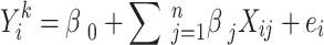
SDSM 6.1 enhances the representation of interannual variability by combining multiple linear regression (MLR) and stochastic weather generator (SWG) techniques⁴⁷; Additionally, SDSM 6.1 integrates regional multiple linear regression (MLR) techniques with more localized climate variables like temperature and precipitation to create statistical relationships between these variables and larger-scale climate forecast variables. Usually, the downscaling procedure needs two kinds of daily data: broad-scale climate predictors from GCM and the corresponding finer-scale climate variables obtained from observed data. The framework describes SDSM 6.1, shown in (Fig. 3). When downscaling daily weather data, a direct relationship is established between the predictand, , and the selected predictor variables, , using the following Eq. (1):

1

Fig. 3.

Detailed step-by-step flowchart for using SDSM 6.1 for statistical downscaling and simulation of future climate data.

Here, k represents a transformation (such as fourth root, inverse normal, or logarithmic), βj denotes the regression coefficient, and represents the model error⁴⁸.

Bias correction techniques

The bias correction was used to address uncertainty arising from the spatial averaging limitations of the GCM of the downscaled temperature and precipitation data by the linear scaling method. Bias correction was implemented using the linear scaling method in the CMhyd software on a daily timescale. The steps included (1) inputting downscaled climate data from the SDSM and daily observational data for each station, (2) defining the calibration and validation period, (3) calculating deviations or ratios between the downscaled and observational data for each month, and (4) applying the corrections to the entire climate data series, to produce corrected data that better reflects reality and is subsequently used in hydrological modeling. During calibration, statistical parameters, including R², RMSE, MBE, and NSE are employed to serve as a reliable measure to evaluate model performance. Details of the bias correction framework are shown in (Fig. 4).

Fig. 4.

Detailed step-by-step framework for using CMhyd1.02 for bias correction of future climate data.

Analysis of results

Accuracy of spatial and temporal GCMs

GCMs are tested to determine how accurately reflect diverse weather patterns in different climate zones. Statistical measures such as correlation coefficients (CC) are used to assess how well the GCMs reflect these patterns. Furthermore, the GCMs’ spatial maps of temperature and precipitation outputs are contrasted with the real observed data. Orographic precipitation and temperature change patterns are difficult for the CMIP6 models to reliably replicate, according to research⁴⁹. This challenge is probably caused by the coarse resolution of the models, which results in irregular climatic patterns, as seen in (Figs. 5 and 6) obtained by using (Arc GIS 10.5). The performance of the models significantly influences the correlation results, which exhibit significant variance within the river basin’s climate zones. The lowest CC values, which dip below 0.43, are found in the driest portions of the river, particularly in desert and hyper-arid zones. On the other hand, coastal regions, especially those in the central and northeastern regions of the river basin, have comparatively higher CC values, which can approach 0.73.

Fig. 5.

Maps of daily precipitation correlation coefficient over ERB compared with observed data represented by using (Arc GIS 10.5).

Fig. 6.

Maps of daily mean temperature correlation coefficient over ERB compared with observed data represented by using (Arc GIS 10.5).

The climate data reveals significant uncertainty and biases among climate models across different climatic zones. For instance, the MRI-ESM2-0 and CNRM-CM6-1 models exhibit fewer biases in humid and dry sub-humid zones but display more substantial biases in arid, semi-arid, and hyperarid regions. In contrast, the BCC-CSM2-MR model demonstrates high accuracy in arid climates, medium biases in semi-arid and hyperarid zones, and very high biases in humid areas. Similarly, CanESM5 shows good consistency in hyper-arid regions, medium biases in arid zones, and very high biases in both semi-arid and humid regions. The HadGEM3-GC31-LL model is considered acceptable, with few biases in semi-arid and moderately rainy areas. However, the CESM2 model exhibits high biases and inadequacies in documenting patterns of rainfall and changes in the distribution of heat in all climatic zones within the basin of the research area between 1982 and 2022. This suggests that the quality of the models varies depending on climatic conditions, showing better correlations in coastal regions and lower correlations in drier areas.

Figures 7 and 8 show the performance of GCM in capturing climate variables under diverse seasonal conditions and the zones for precipitation and temperature, respectively. In these figures, the bottom bar in each panel illustrates observations that reveal seasonal biases in temperature variations and precipitation patterns. The results illustrate significant biases in the seasonal precipitation data estimated by almost all climate models. The models underestimate precipitation in rainy areas (humid panels). Conversely, nearly all models systematically underestimate summer precipitation in the humid zone. However, in the arid zone, most models reasonably simulate summer rainfall. Furthermore, there are low biases in the seasonal temperature data estimated by almost all models across all climate zones.

Fig. 7.

Stacked bar charts representing the seasonal distribution of annual precipitation across climatic zones for periods (1982–2022).

Fig. 8.

Stacked bar charts representing the seasonal averages of annual temperature for visual comparison across climatic zones for periods (1982–2022).

Figures 9 and 10 obtained by using (Axcel, 2023) to display the long-term precipitation and temperature anomalies after eliminating each time series’s overall mean to align the means of the all-time series with the observations, ensuring consistency and enhancing accuracy. For precipitation anomalies, high-elevation zones indicate wet periods (above-average rainfall), while low-elevation zones indicate dry periods (below-average precipitation). On the other hand, for temperature anomalies, high areas represent dry periods (above-average temperature), and low areas indicate wet periods (below-average temperature). Since CMIP6 outputs are not constrained by actual historical forcing, an exact match between the wet and dry periods observed in the data cannot be anticipated. However, some model simulations for temperature anomalies show consistency with observations concerning durations and amplitudes of events, although not necessarily their timing. Conversely, wet and dry durations for rainfall anomalies differ substantially from most models’ observations.

Fig. 9.

Annual precipitation anomalies in the study area based on the outputs of GCMs during the period 1982–2022.

Fig. 10.

Annual temperature anomalies in the study area based on the outputs of GCMs during the period 1982–2022.

Performance (SDSM 6.1) downscaling model

The SDSM model was calibrated using multiple regression equations, using observed climate data as predictor variables and elements from GCMs without prior constraints. This step revealed moderate correlations between local weather variables and regional climate elements, such as atmospheric pressure and relative humidity, enhancing the model’s reliability in representing climate dynamics at the local and regional levels. The study relied on a time series of observational data spanning 41 years; 31 years were used for model calibration and 11 years for validation. Two climate variables, precipitation, and temperatures, were focused on as predictor outputs. A simple multiple linear regression model was applied to evaluate the statistical downscaling process, and the calibration results (Fig. 11) showed a remarkable agreement between the simulated values ​​and the actual monthly climate averages, particularly about temperature. However, rainfall results showed higher variability and skewness than temperatures, indicating that rainfall forecasting remains more complex due to its high natural variability and sensitivity to several subtle local factors. Regarding model validation, climate downscaling results across five different climate zones (Fig. 12) showed good agreement between predicted and actual values ​​at most stations. This demonstrates the model’s effectiveness in simulating regional climate behavior when used in future climate change studies

Fig. 11.

Calibration of downscaling (a) precipitation and (b) mean temperature for periods (1982–2011) across climatic zonation.

Fig. 12.

Validation of downscaling (a) precipitation and (b) mean temperature for periods (2012–2022) across climatic zonation.

.

Performance of CMhyd bias correction

Downscaled climate data before applying bias correction as shown in (Fig. 13) showed a clear pattern of bias in the representation of precipitation and temperature. This bias was observed unevenly across different climate regions, with values ​​being underestimated in humid regions and overestimated in arid regions, indicating inconsistent model performance across different climate regions before processing.

Fig. 13.

Statistical index performance of downscaled GCMs precipitation data before and after bias-correction.

Significant variation was also observed in the representation of daily values, particularly in regions with complex terrain. This reflects the limited spatial and temporal resolution of the outputs of some GCMs when used directly without modification. These differences underscore the need to apply bias correction techniques to improve the reliability of the results.

After applying the bias correction procedure, the agreement between simulated and observed values ​​improved significantly, as evidenced by the statistical indicators of rainfall, which showed a marked improvement in all studied climate regions. (R² ranged from 85 to 93%, while NSE ranged from 83 to 92%. RMSE and MBE values ​​decreased, indicating improved model accuracy and reduced systematic deviations in the estimation, as shown in (Fig. 14).

Fig. 14.

Statistical index performance of downscaled GCMs temperature data before and after bias-correction.

It should be noted that the statistics presented represent the average performance of a selected set of general climate models after applying statistical downscaling and bias correction, which were calculated across different climate regions. However, this section does not present the pre-correction statistical values in detail. Therefore, a direct quantitative comparison between the pre-and post-correction statistics is recommended to more clearly demonstrate the effectiveness of this procedure and enable the reader to assess the extent of the model performance improvement.

Projection future precipitation

The cumulative results of the relative precipitation change (2024–2100) as shown in (Fig. 15) reveal significant variation across the different climatic zones within the Euphrates Basin under the three climate scenarios: SSP1-2.6, SSP2-4.5, and SSP5-8.5. The figure shows that the precipitation response to climate change is not uniform but varies depending on the scenario intensity and climatic zone. In humid and sub-humid regions, SSP1-2.6 shows significant increases in precipitation, with positive changes in some humid locations reaching approximately + 17%, reflecting a positive climate response under ambitious climate action. SSP5-8.5, despite being a high-emission scenario, also recorded a relative increase of approximately + 4%, indicating that some areas of this basin may continue to receive relatively high rainfall rates even under severe climate change due to increased ocean evaporation and moisture transport.

Fig. 15.

Projections of precipitation for the period 2024–2100 across climatic zonation within ERB under emission scenarios SSP1-2.6, SSP2-4.5, and SSP5-8.5.

In contrast, semi-arid and arid regions experienced progressive precipitation declines across scenarios. For example, the arid region south of the basin (around the Haditha reservoir) showed a cumulative decline of approximately − 7% under SSP1-2.6, increasing to −9% under SSP2-4.5 and reaching approximately − 18% in SSP5-8.5. This trend reflects the continuing deterioration of these regions’ hydrological capacity. It is consistent with regional projections of increased drought intensity and reduced hydrological cycle efficiency under future warming.

Time-wise, the data (as shown in the text associated with Fig. 15) show that the mid-century period (2041–2070) represents a critical turning point, with precipitation beginning to decline more markedly than the short-term period (2024–2040), particularly in the SSP2-4.5 scenario, which represents a medium trajectory and is commonly used for climate planning. This gradual decline in precipitation coincides with increased seasonal variability. Models indicate a slight increase in winter precipitation compared to a significant decrease in summer precipitation, causing an imbalance in water availability. These results clearly indicate the heterogeneous climate change affecting the Euphrates River Basin and increasing the risk of prolonged or seasonal drought, especially in light of increasing water demand in the coming decades. This highlights the urgent need to develop flexible water management strategies based on multiple scenarios, focusing on securing supplies during dry seasons and increasing the efficiency of using available resources.

Figures 16 and 17 show that future precipitation changes under different emission scenarios (SSP1-2.6, SSP2-4.5, and SSP5-8.5) exhibit apparent variations in direction and magnitude. According to the bar chart, SSP2-4.5 indicates the most significant relative cumulative decrease in mean precipitation compared to the historical period, exceeding − 6% in some locations, while SSP1-2.6 and SSP5-8.5 showed moderate increases. The box plot allows visualization of the statistical distribution of precipitation changes among climate models, showing a widening range of change under SSP5-8.5 and a steepening of the overall trend line, indicating a gradual decrease in projected precipitation amounts as the scenario becomes more severe. These results highlight the importance of considering intermodal variability and not simply relying on the average. They also confirm that future climate impacts on precipitation will not be uniform across spatial scenarios. The extracted numerical values ​​are referenced in the text and directly linked to the figures to facilitate tracking and verification.

Fig. 16.

A cumulative variation (%) in mean precipitation under three emission scenarios over the Euphrates River region.

Fig. 17.

Relative change in average precipitation (%) compared to the historical period under three emission scenarios (SSP1-2.6, SSP2-4.5, SSP5-8.5).

Projection future temperature

Climate correction indicates that future temperatures will rise across various climatic zones, as illustrated in (Fig. 18). This trend is especially pronounced under high-emission scenarios, which suggest a significant warming trend affecting temperature patterns. (Fig. 19) displays the absolute change in average annual temperature, showing expected increases under the SSP 2-4.5 and SSP 5–8.5 scenarios. In the 2070 s, the projected temperature rises are higher, 2.26 °C for SSP 2-4.5 and 3.15 °C for SSP 5-8.5, compared to the 2040 s, where the increases are 1.9 °C and 2.5 °C, respectively. By the 2090 s, the temperature increases become even more pronounced, with projections of 3.0 °C and 4.8 °C under SSP 2-4.5 and SSP 5-8.5, respectively, as shown in (Fig. 20). Furthermore, the temperature rise is expected to be significantly more significant under the SSP 5–8.5 scenario, suggesting that continued growth in greenhouse gas emissions will further elevate temperatures. The CMIP6 models project a notable temperature increase across several sub-basins of the ERB. Seasonally, the increase in temperature during winter is anticipated to be minimal, averaging about 1.8 °C. In contrast, maximum summer temperatures are projected to rise significantly, particularly in hyper-arid regions. This overall temperature increase reflects the warming effect of surface water near the downstream areas.

Fig. 18.

Projections of temperature for the period 2024–2100 across climatic zonation within ERB under emission scenarios SSP1-2.6, SSP2-4.5, and SSP5-8.5.

Fig. 19.

A cumulative variation (%) in mean temperature under three emission scenarios over the Euphrates River region.

Fig. 20.

Relative change in average temperature (%) compared to the historical period under three emission scenarios (SSP1-2.6, SSP2-4.5, SSP5-8.5).

Discussion and Conclusions

This study utilized a modification technique known as Statistical Downscaling and Bias Correction to analyze a temperature and precipitation dataset generated by GCMs from the CMIP6 project. Additionally, it assessed the uncertainties associated with GCMs and projected future trends in precipitation and temperature under three different emission scenarios (SSPs). The following is a summary of the key conclusions and discussion:

1. The accuracy of the selected GCMs to capture the spatial and temporal climate patterns under their inherent errors and uncertainty biases for the future development of a suite of CMIP6 models was determined as follows: (i) Spatial biases in rainfall and temperature ranged from (−40 ~ 37) and (−34 ~ 34 mm). In contrast, spatial CC ranges (0.18 ~ 0.47) and (0.36–0.81), respectively, show that there are considerable differences in the CMIP6 models’ performance across the various climatic zones. (ii) The variation of precipitation patterns and temperature distribution in most GCMs exhibits notable discrepancies of about (25%) of the corresponding values in the observations, where it tends to underestimate the average annual precipitation while overestimating the average minimum and maximum temperatures. (iii) The biases of climate model simulations showed substantial variation across five climatic zones (low CC) values, whereas in humid and dry sub-humid zones, CNRM-CM6-1 and MRI-ESM2-0 work rather well. However, their performance faltered in hyper-arid and semi-arid areas. Conversely, HadGEM3-GC31-LL, BCC-CSM2-MR, and CanESM5 exhibited more favourable performance in semi-arid, arid, and hyper-arid zones but weaker performance in humid zones. (iv) Based on these results, the high uncertainties in the CMIP model limit the reliability of the projection of climate data. Therefore, the choice of the GCMs as individual models is better than linear trends to mitigate climate variable uncertainty biases across several climatic zones.

2. The SDSM 6.1 statistical downscaling approach to GCM grid output covering the study area through calibration-validation results gave acceptable agreement with the existence of disparities between observed and predicated data due to limitations in projecting climate index magnitude and spatial patterns. Therefore, the linear scaling of the bias correlation showed a significant improvement in GCM data projection.

3. The linear scaling techniques of the bias correlation to process daily outputs of projected downscaling temperature and precipitation dataset from GCMs using CMhyd showed a significant improvement, where the statistics metrics performance values of (R2, NSE, RMSE, and MBE) were 0.79, 0.82, (0 ~ 4) °C, and (−2 ~ 8) % for max temperature, 0.84, 0.83, (0 ~ 2.1) °C, and (−2 ~ 3) % for min temperature, and 0.89, 0.88, (10 ~ 185) mm, and (−0.2 ~ −0.7) % for precipitation respectively.

4. The changes in the prediction of precipitation within the study area varied based on the climatic zone under (SSP 1-2.6, SSP 2-4.5, and SSP 5-8.5) as follows:

• Humid and dry-subhumid zones experienced increased precipitation of (17.74%, 9.25%, and 4.61%) (8.61%, 5.25%, and 2.61%) respectively.

• The semi-arid, arid, and hyper-arid zones are expected to decrease where the arid region at Haditha reservoir location reaches (−7.04%, −9.25%, and − 18.61%), respectively.

• The annual precipitation at the Euphrates River basin is projected to decrease in the 2040 s to 2099 s, indicating a severe drought and a more pronounced precipitation anomaly towards the 21 st century over most parts of the basin. The intensity may vary from one sub-basin to another, which agreement previous studies.

• Most monthly precipitation (> 85%) occurs during the wet season from November to April, while the remaining months are characterized by a dry season, with precipitation accounting for less than 15% where most climate models generally agree on a reduction in precipitation in summer and an increase in winter.

• 5.The selected GCMs projected a rise in future temperatures in varying proportions over the entire climatic zone, which suggests that the continued increase in GHG emissions will lead to a further rise in temperature as follows:

• The absolute change in average annual temperature is an increment under both SSP 2–4.5 and SSP 5–8.5 scenarios (1.9 °C and 2.5 °C) in 2040 s (2.26 ◦C and 3.15 ◦C) in 2070s.

• In the subsequent 2090 s, the projected increases are more substantial, with temperature rises of 3.0 °C and 4.8 °C under SSP2-4.5 and SSP5-8.5, respectively.

• The maximum summer temperature is projected to rise, especially in hyper-arid regions. This increase in temperature suggests that heating the surface water near the downstream point leads to the warming effect.

Supplementary Information

Below is the link to the electronic supplementary material.

Author contributions

Halah Kadhim Tayyeh: data curation, formal analysis, investigation, methodology, project administration, resources, software, writing the original manuscript, Writing and reviewing the manuscript and final approval of the version to be published, Ruqayah Mohammed: Supervisor, Amnah Alasqah: Funding, Ahmed Mageed Hussein: Calibration and validation software, Khaled Mohamed Khedher: Reviewing the manuscript, Brahim Benzougagh: Reviewing the manuscript.

Funding

This research was funded by the Deanship of Scientific Research at Princess Nourah bint Abdulrahman University Researchers Supporting Project number (PNURSP2025R668), Princess Nourah bint Abdulrahman University, Riyadh, Saudi Arabia.

Data availability

All data generated or analyzed during this study are included in this manuscript and its supplementary information files of this study are available on Zenodo under license with restricted access. 10.5281/zenodo.14983548

Declarations

Competing interests

The authors declare no competing interests.