Development of data driven models to accurately estimate density of fatty acid ethyl esters

Abstract

Fatty acid ethyl esters (FAEEs) are widely used in biofuels, pharmaceuticals, and lubricants, offering an eco-friendly alternative due to their biodegradability and renewable nature, contributing to environmental sustainability. The objective of this study is to construct advanced predictive algorithms using various machine learning methods, including AdaBoost, Decision Trees, KNN, Random Forests, Ensemble Learning, CNN, and SVR. These models aim to accurately predict the density of FAEEs across different temperature, pressure, molar mass, and elemental composition (oxygen, carbon, and hydrogen content). Experimental data reported in earlier publications were employed to develop the models. Results indicate that the dataset is highly well-suited for developing reliable models based on data. Analysis reveals that temperature exerts a considerable influence on density, with pressure also playing a critical role. The reliability of the dataset, consisting of 1307 experimental datapoints gathered from the literature, was ensured through the application of a Monte Carlo outlier detection algorithm, which validated its suitability for model training and validation. Through extensive statistical evaluations and visualization techniques, SVR emerged as the most accurate model for density prediction. Sensitivity analysis confirms the influence of all input features, with SHAP analysis identifying temperature as the most dominant factor affecting density. The developed framework provides an economical and time-saving substitute for laboratory-based experimentation density measurements, enabling precise density estimation for FAEEs under various conditions.

Introduction

The increasing worldwide need for sustainable and environmentally friendly energy solutions has intensified research into renewable alternatives. In this context, fatty acid ethyl esters (FAEEs) have appeared as encouraging options for biofuels due to their renewable nature, biodegradability, and favorable physicochemical properties. FAEEs are widely utilized in biofuel production, pharmaceuticals, and industrial applications, offering a cleaner alternative to conventional fossil fuels^1,2. Their low toxicity and compatibility with existing fuel infrastructure further enhance their viability as a sustainable energy source. Additionally, FAEEs contribute to environmental sustainability by decreasing emissions of greenhouse gas and lessening the ecological effects of energy generation.

Liu et al. executed research on viscosities and densities of ethyl heptanoate and ethyl octanoate within a temperature span of 303–353 K and pressures attaining up to 15 MPa. Their findings demonstrated that density displayed an increasing trend with pressure and a decreasing trend with temperature³. This research contributes valuable experimental data to further our understanding of thermophysical properties of FAEE. Wang et al. carried out a research on densities of pure ethyl octanoate and its mixtures with n-hexadecane within a temperature range of 293.15 K to 363.15 K and pressures reaching up to 60 MPa. They employed a U-shape vibrating-tube densimeter for the measurements⁴. The study achieved precise density predictions with deviations below 0.52%, thus contributing important knowledge about the characteristics of FAEEs. Ndiaye et al. conducted a research on sound speed in ethyl caprate and methyl caprate under various pressure conditions, ranging up to 210 MPa, and temperatures between 283.15 and 403.15 K. They also performed density measurements at pressures reaching 100 MPa and extended density values for higher pressures⁵. Their research offered valuable insights into the thermophysical properties of FAEE, like isentropic and isothermal compressibilities, thus expanding our understanding of these substances.

Wang et al. carried out a research analysis on the density of ethyl laurate and methyl laurate through the application of an oscillating-tube density measurement device. The assessments were conducted within a temperature range of 283.15 to 363.15 K and pressures up to 60 MPa⁶. The study also included calculations of thermodynamic properties like isothermal thermal expansivity and compressibility, further enhancing our understanding of the density behavior of fatty acid ethyl esters. He et al. conducted a study on viscosity and density of ethyl dodecanoate and methyl dodecanoate within a temperature range of 302–354 K and pressures up to 15.2 MPa⁷. This research provides useful perspectives into the pressure and temperature-dependent properties of biodiesel components, thereby contributing to a deeper understanding of these materials.

Habrioux et al. conducted a study on density, compressibility, sound speed, and viscosity of ethyl methyl and laurate laurate in liquid form. The assessments were conducted within a pressures reaching 200 MPa and a temperature span of 293.15 to 353.15 K. Acoustic wave sensors and pulse-echo techniques were utilized to measure density through the Newton-Laplace Eq.⁸. This research provides important data on thermophysical characteristics of fatty acid ethyl esters in high-pressure environments, contributing to our overall understanding of these substances. Aissa et al. carried out an investigation into speeds of sound, densities, viscosities, and refractive indices of various fatty acid esters, among which was ethyl laurate. The measurements were carried out over a broad spectrum of pressures and temperatures⁹. This research offers valuable thermophysical data, emphasizing the differences in density and compressibility between methyl and ethyl esters, and contributes to our overall understanding of these substances.

Ndiaye et al. carried out a research on sound speeds and densities of fatty acid esters, with ethyl myristate being one of the investigated substances. The measurements covered an extensive range of temperatures and pressures¹⁰. The study resulted in an equation of state that precisely predicts speed of sound and density, thus offering significant insights into the thermophysical characteristics of FAEE.

Tat and Van Gerpen conducted a study on sound speed, isentropic bulk modulus, and density of biodiesel and its pure ester constituents across a range of temperatures and pressures. Their research shed light on the significance of these properties, as they impact fuel injection timing and, consequently, may affect engine performance and emissions¹¹. The variations in density and speed of sound may lead to timing advances, which could potentially influence NOx emissions in biodiesel-fueled engines. Their findings suggest that understanding these properties is crucial for optimizing fuel injection strategies and minimizing emissions in biodiesel-powered engines. Recently, Sukpancharoen et al. employed machine learning algorithms for estimating the output of biodiesel produced through transesterification reactions using various catalyst types, including homogeneous, heterogeneous, and enzymatic ones. Their study highlights the effectiveness of computational approaches particularly extreme gradient boosting in capturing complex relationships in biofuel production systems¹². Rermborirak et al. developed a an affordable and compact system for identifying microplastics, combining Nile Red dyeing techniques with a YOLOv8-driven deep learning framework, demonstrating the practical feasibility and cost-effectiveness of machine learning tools in real-world analytical applications¹³. Their work exemplifies how advanced computational methods can significantly reduce operational costs while maintaining high predictive accuracy an approach that aligns with the objectives of our FAEE density prediction framework.

Over the past few years, the incorporation of machine learning techniques into renewable energy systems has advanced rapidly, offering promising alternatives to traditional modeling techniques^14–19. Within the biodiesel research domain, ML has been widely applied to optimize and predict key outcomes such as yield, purity, and performance. For instance, several studies have explored the use of ML to forecast biodiesel yield based on variables like catalyst type, feedstock composition, and reaction parameters, achieving high predictive accuracy^20,21. Additionally, artificial neural networks (ANNs) have demonstrated excellent performance in estimating engine behavior and emissions from biodiesel-diesel blends²². Recent developments have also combined ML with optimization methods such as response surface methodology (RSM) and evolutionary algorithms to improve biodiesel output and reduce environmental impact^23,24. Despite these advances, limited studies have focused specifically on the density prediction of FAEEs, which is a critical thermophysical property influencing fuel transport, injection timing, and combustion.

Despite these advantages, the precise prediction of FAEE density continues to pose a major obstacle owing to the intricate nature of interactions between temperature, pressure, molar mass, and elemental composition (oxygen, carbon, and hydrogen content). Density is a critical parameter that influences fuel performance, combustion efficiency, and transport properties, making its accurate estimation essential for industrial applications. Experimental density measurements, while reliable, are often time-consuming and resource-intensive, necessitating the development of efficient computational models for rapid and precise predictions. This study seeks to address this limitation through the creation of sophisticated machine learning frameworks (Decision Trees, AdaBoost, Random Forests, KNN, Ensemble Learning, CNN, and SVR models) to accurately predict FAEE density, leveraging a refined dataset of 1307 data points. An anomaly detection algorithm (Monte Carlo Outlier Detection (MCOD) algorithm) was applied to guarantee the integrity of data reliability, and an analysis of input variable importance was performed to evaluate how each factor influences density of FAEEs. A range of evaluation indicators and graphical methods were applied to assess how precisely the models predicted the target values. Furthermore, SHapley Additive exPlanations (SHAP) analysis was employed to interpret the impact on key features on density predictions, offering meaningful understanding of the role of elemental composition, molar mass, temperature, and pressure. The overall methodology is illustrated in Fig. 1. The present work addresses this gap by systematically evaluating multiple ML algorithms to model FAEE density using a broad dataset that incorporates temperature, pressure, molar mass, and elemental composition. By doing so, it extends existing efforts in biodiesel-related ML modeling beyond yield estimation and into the accurate prediction of transport-relevant physical properties.

Fig. 1.

Methodology for identifying the most effective model based on data-driven approaches.

Summary of methods employed in the field of machine learning

Decision tree (DT)

DT method represents a widely adopted approach within supervised learning frameworks for classification and regression jobs. It iteratively partitions data based on various features, creating a hierarchical model in which every branching point denotes a decision rule, and each terminal node corresponds to a prediction. Metrics like information gain, Gini impurity, or variance reduction are employed to establish the optimal feature for data partitioning, depending on the problem’s nature^25,26. The Gini impurity for a dataset can be calculated as:

1

Where D is databank, n is classes number, and p_i is probability of an instance belonging to class i. Similarly, information gain is calculated as:

2

where D represents databank, A denotes feature, Values(A) indicates potential feature A values, and D_v is subset of D where feature A has value v, and Entropy(D) is the entropy of the dataset D.

One of the key advantages of DT lies in their exceptional ease of interpretation. The resulting model is easy to visualize and comprehend, making it an ideal resource in situations where transparent reasoning behind decisions is essential^27,28. Despite their simplicity and interpretability, Decision Tree algorithms possess both strengths and limitations.

Benefits include reduced need for data preprocessing, the ability to handle numerical and categorical data, and some resilience against outliers^29,30. Additionally, the algorithm inherently identifies nonlinear relationships between features without requiring complex transformations. However, a significant challenge of Decision Trees is their tendency to overfit, particularly when trees become too deep or complex, leading to poor performance on new datasets^31,32. Techniques such as tree pruning, setting a maximum depth, or employing ensemble algorithms like gradient boosting and random forests can reduce overfitting issues. While Decision Trees may not achieve the accuracy of more advanced algorithms, their ability to offer transparent understanding of the decision-making process makes them a valuable asset in fields like medicine, finance, and marketing^33,34.

Adaptive boosting

AdaBoost is a modern ensemble-based classification algorithm within machine learning field^35,36. The central concept underpinning AdaBoost involves the strategic combination of multiple weak learners, often decision trees, to develop a robust and adaptable learning algorithm³⁷. By amalgamating individual learners, AdaBoost can achieve enhanced predictive performance and robustness compared to standalone models^38,39. The algorithm operates by allocating weights to every training instance and iteratively adjusting these weights based on the errors of the weak learners. The weight update rule for each instance is given by:

3

where: w_i(t) indicates the assigned weight of the ith data point at iteration t, α_t refers to the contribution weight of the weak classifier h_t during the same iteration, y_i stands for the true label associated with the ith observation, and h_t(x_i) denotes the predicted output from the weak learner h_t for that observation. The value of α_t, determining the influence of each weak learner, is computed using the following expression^40,41:

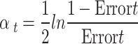4

Where Error_t​ is the weak learner’s weighted mistake h_t​ at iteration t.

AdaBoost effectively addresses clustering and overfitting challenges by intelligently integrating weak learners, resulting in a versatile and precise prediction model^42,43. This approach allows AdaBoost to harness the unique advantages offered by each base model while minimizing their limitations, leading to improved overall performance.

Random forest

Random Forest, a prominent Ensemble Learning method, integrates numerous decision trees to achieve precise predictions^44,45. Each individual tree within the ensemble is built separately by drawing random samples from both the feature space and the training dataset⁴⁶. The overall output of a Random Forest model is obtained by combining the results generated by all constituent decision trees. In classification problems, this aggregation usually involves selecting the most frequently predicted class (majority vote), whereas in regression scenarios, the mean value of all tree outputs is taken as the final prediction. Mathematically, the final regression estimate can be formulated as follows:

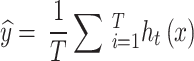5

In this equation, ŷ denotes the aggregated output, T refers to the total number of decision trees within the ensemble, and h_t​(x) corresponds to the prediction generated by the t-th tree for the input instance x.

This ensemble strategy enables Random Forest to leverage the predictive capabilities of multiple models while mitigating overfitting and enhancing generalization performance^47,48. The utilization of random subsets and features in Random Forest results in a model that exhibits both precision and resilience, while effectively minimizing overfitting risks^49,50. Overfitting, a common challenge where a model exhibits strong performance during training yet struggles with unseen data during testing, is mitigated through Random Forest’s ensemble approach^51–53. By combining multiple decision trees, Random Forest reduces the reliance on individual models and effectively captures patterns and relationships within the data^54,55.

Ensemble learning (EL)

EL is widely recognized in statistics and machine learning for combining several models to produce a single, unified prediction from a dataset^44,45. This approach involves several algorithms working together to generate individual predictions, which are then combined to produce the ultimate result^56,57. Although the most frequent output is often selected as the final prediction, different ensemble learning models may assign varying weights to individual predictions or adopt a sequential approach, utilizing the outputs of previous models^58,59.

For instance, under a weighted voting scheme, the ultimate decision ​ can be calculated as:

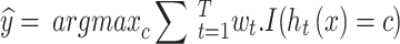6

where: T denotes the total number of models within the ensemble, w_t​ indicates the weight allocated to the tth model, h_t​(x) is the output of the t-th model for the input x, I(·) represents an indicator function that yields 1 if the specified condition holds true and 0 otherwise, and c refers to the set of possible class labels^59,60.

Convolutional neural networks (CNNs)

CNNs represent a category of deep learning models specifically designed to process structured inputs, particularly visual data like images. By utilizing convolutional layers, these models are capable of identifying spatial patterns such as contours, surface details, and geometric forms within the input⁶¹. The convolution operation in a CNN can be mathematically represented as:

7

Within this framework, f refers to the input image or intermediate feature map, g designates the convolutional filter applied during the operation, and (x, y) specifies the spatial location within the resulting activation map⁶².

One significant advantage of CNNs is their effectiveness in handling data with many dimensions, making them well-suited for tasks such as identifying objects and classifying images. These models often incorporate pooling layers to reduce feature map size and mitigate the risk of overfitting. Due to their impressive accuracy, CNNs have had a profound impact on advancements in computer vision⁶³.

K-nearest neighbors (KNN)

KNN method is a straightforward yet effective approach within the supervised learning technique applied to regression and classification jobs. It functions on the similarity basis, identifying value or class of a data point by looking at the most common class or the average value of its (k) nearest neighbors in feature space^64,65. The method measures the distance from the target point to every other point in the dataset, usually employing metrics like Euclidean distance, which can be expressed as^66,67:

8

In this formulation, x and y represent two samples within the feature space, n indicates the total number of features, and x_i and y_i correspond to the values of the i-th feature for data points x and y, respectively.

KNN operates as a non-parametric method, meaning it makes no assumptions about the data’s underlying distribution. This characteristic grants it adaptability, making it applicable to a wide range of data structures^68,69. One of the main advantages of the K-Nearest Neighbors (KNN) algorithm is its simplicity and ease of implementation. However, its performance is highly sensitive to the choice of the parameter k and the distance measurement used. Selecting a small k may cause the model to overfit the training data, while a larger k can lead to underfitting by oversmoothing the decision boundaries⁷⁰. Moreover, KNN can be resource-intensive for extensive datasets since it necessitates computing distances between the target point and every other point in dataset. In spite of these difficulties, KNN is commonly utilized in areas like recommendation systems, image identification, and medical diagnostics, due to its straightforward approach and efficiency in identifying local patterns in data^71,72.

Support vector machine (SVM)

Support Vector Machine (SVM) is a robust machine learning technique for regression and classification jobs, established on statistical learning principles and nonlinear optimization. SVM operates by identifying an ideal hyperplane (support vector) that divides two or more sets of data^73–75. The fundamental principle of this approach is to maximize distance between training data points and decision boundary (Margin Maximization), thereby improving the model’s capability to generalize. Mathematically, the optimization task for SVM can be expressed as:

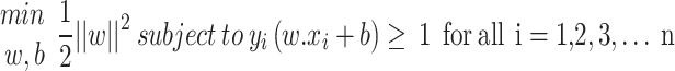9

In this setting, w defines the hyperplane’s weight vector, b is the bias constant, x_i denotes the ith input sample, y_i corresponds to its associated class label (either + 1 or − 1), and n represents the complete count of samples in the dataset^76–78.

When the data cannot be separated linearly, SVM employs kernel functions like Gaussian or polynomial kernels to convert the information into a more complex-dimensional space, enabling for better separation^79,80. One of the primary strengths of Support Vector Machines (SVM) is their ability to handle datasets with many features, making them highly effective for applications like visual recognition and language processing tasks. Nonetheless, a significant obstacle of this algorithm is its computational complexity and extended processing duration for sizable datasets^81,82. Moreover, adjusting model parameters like the kernel type, penalty parameter (C), and parameters specific to the kernel necessitates substantial experimentation and cross-validation methods. In spite of these constraints, SVM continues to be a key algorithm in machine learning because of its excellent accuracy and adaptability across different applications^83,84.

Information collection and performance assessment metrics

Overview of the data acquisition process

The information required for developing the machine learning models in this study was obtained based on findings reported in earlier studies that conducted extensive experimental analyses on the density characteristics of various FAEEs under different laboratory conditions. The dataset includes 1307 data points, incorporating key input variables such as temperature, pressure, molar mass, and elemental composition (oxygen, carbon, and hydrogen content)^3–11. The FAEEs considered in this study include: Ethyl caprate, Ethyl dodecanoate, Ethyl heptanoate, Ethyl laurate, Ethyl linoleate, Ethyl myristate, Ethyl octanoate, Ethyl oleate, and Ethyl stearate. Table 1 presents the range of temperature, pressure, and density values for each fatty acid ethyl ester (FAEE) included in this study. The dataset covers a broad spectrum of thermodynamic conditions, with temperatures ranging from 283.15 K to 413.15 K and pressures extending up to 200 MPa. This wide variation ensures that the machine learning algorithms are trained on diverse scenarios, enhancing their generalizability and robustness. The density values also span a significant range, reflecting differences in molecular structure and composition among the FAEEs, which reinforces the demand for highly reliable forecasting tools capable of capturing such complex variations.

Table 1.

Temperature, pressure, and density ranges for the studied fatty acid Ethyl esters (FAEEs).

FAEE name	Temperature range (K)	Pressure range (MPa)	Density range (kg/m3)
Ethyl Caprate	293.15-393.15	0.1013-100	780.8-916.4
Ethyl Linoleate	293.15-373.15	0-34.5	831–903
Ethyl Myristate	293.15-393.15	0.1013-100	784.5-904.4
Ethyl Stearate	313.15-373.15	0-34.5	807-869.8
Ethyl Dodecanoate	303.06–353.2	0.1-15.04	815.3-864.5
Ethyl Laurate	293.15-413.15	0.1–60	767.0-894.7
Ethyl Myristate	293.15-413.15	0.1–60	769.4-889.4
Ethyl Oleate	293.15-413.15	0.1–60	781.3-899.2
Ethyl Heptanoate	303.1-353.23	0.1-15.15	815.1-877.5
Ethyl Laurate	283.15-363.15	0.1–200	807.52–927.7
Ethyl Octanoate	293.15-363.15	0.1–60	805.66-903.44

In this study, density is treated as the primary output variable, whereas temperature, pressure, molecular weight, and the elemental percentages of oxygen, carbon, and hydrogen are considered the main predictors. To explore the impact of these variables on FAEEs density and to assess their range and behavior, visual correlation plots have been generated and are presented in Fig. 2. These visual tools offer an in-depth perspective of the dataset, highlighting patterns, inter-variable relationships, and potential anomalies. This exploratory step plays a key role in understanding the dataset’s underlying structure and supports the creation of robust forecasting algorithms. Furthermore, Fig. 3 illustrates raincloud diagrams for every parameter individually, enabling a clear view of their distribution characteristics.

Fig. 2.

Scatter matrix visualization illustrating the interdependencies among the variables.

Fig. 3.

Visualization of variable distributions using raincloud plots.

To enhance the accuracy of machine learning algorithms, the K-fold cross-validation technique was applied, which allows the entire dataset to be systematically leveraged for evaluation over K iterations^85–87. This method involves dividing the dataset into K equally sized segments, with each fold serving a single time as the validation set, and the other K–1 portions serve for model training. After all K cycles are completed, the validation results are combined to yield a more stable and unbiased performance estimate, reducing the effects of randomness in data partitioning. Additionally, this strategy significantly lowers the risk of overfitting. In this study, each machine learning model was trained using a five-fold cross-validation scheme to enhance its ability to generalize to unseen data.

Performance metrics for assessing model accuracy

In order to evaluate and compare the effectiveness of each constructed machine learning model in handling prediction tasks, several key performance indicators are calculated for each algorithm, including^13,88–90:

Relative error percent:

10

Average absolute relative error:

11

Mean square error:

12

Determination coefficient:

13

In the given formulas, the subscript i refers to the index corresponding to a specific observation within the databank. The abbreviations pred and exp indicate the predicted and measured values for every respective entry. Furthermore, N signifies the total number of data instances contained in the dataset^91–93.

The predictive models are constructed using a set of input features that include temperature, pressure, molecular weight, and the elemental composition specifically the percentages of oxygen, carbon, and hydrogen. The output variable to be predicted is the density of FAEEs. For a comprehensive evaluation of model performance, databank is randomly split into three distinct portions. The majority of the data (90%) is allocated for training purposes, while the remaining 10% is reserved for testing.

To reduce the influence of variation within the dataset, all input and output variables are scaled using a standardization formula prior to training the models. This preprocessing step addresses differences in units and value ranges among the features, enhancing the models’ ability to produce consistent and precise predictions. Normalizing the data enables the algorithms to detect meaningful trends and associations more efficiently while minimizing the dominance of specific variables. The standardization equation is given below:

14

In the normalization formula, the symbols represent the following: n refers to the original, unprocessed data value; n_max and n_min denote the maximum and minimum values within the dataset, respectively; and n_norm indicates the resulting standardized value.

Results and analysis

Identification of anomalous data points

Before constructing data-driven algorithms to estimate density of fatty acid ethyl esters (FAEEs), it is crucial to ensure data reliability by addressing outliers. This study employs the Monte Carlo Outlier Detection (MCOD) algorithm, which efficiently detects anomalies in large datasets by combining random sampling with density-based techniques. MCOD identifies local density variations to highlight points that significantly deviate from their surrounding values. By leveraging Monte Carlo sampling, the algorithm evaluates a subset of the data, reducing computational costs while maintaining accuracy⁹⁴. Due to its ability to scale effectively and operate with high speed, it is well-adapted for use in real-time environments and with datasets containing a large number of features. However, like any method, MCOD requires a trade-off between precision and computational efficiency, affected by elements like dataset magnitude and the selected count of closest neighbors (k). Even with these factors in mind, MCOD remains a valuable method for preliminary data exploration and identifying unusual patterns, especially when precise accuracy is not critical or when processing power is constrained.

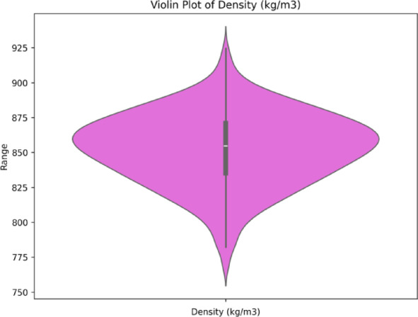
Figure 4 displays a boxplot that visualizes the dataset applied in this investigation, highlighting the spread of FAEE density values and establishing the permissible boundaries for model training. The concentration of data points within the defined limits suggests strong data integrity. In this work, the entire dataset was employed throughout the model learning process using machine learning techniques algorithms, promoting the development of models grounded in a complete and well-balanced sample. This strategy improves the models’ capacity to generalize across new inputs by effectively learning the intrinsic trends and fluctuations in the data. Consequently, the models demonstrate improved precision and robustness in predicting the density of FAEEs.

Fig. 4.

(A) Identifying outliers using the monte carlo algorithm, (B) Boxplot of data distribution.

Sensitivity analysis

In this part of paper, the influence of temperature, pressure, molecular weight, and elemental makeup on the density of FAEEs is examined. The analysis also includes evaluating the comparative influence exerted by each variable. To measure the importance of these variables, a relevance factor is calculated using the equation provided below⁹⁵:

15

Within this framework, the subscript j refers to the particular feature under examination. The relevance factor ranges between − 1 and + 1, where values approaching + 1 reflect a strong positive link between the input and the target variable. On the other hand, values closer to − 1 imply a strong inverse association. A negative score reveals that the input and output move in opposite directions, while a positive score denotes a direct relationship.

As shown in Fig. 5, correlation matrix illustrates the interdependencies among the input features pressure, temperature, molar mass, and elemental composition (oxygen, carbon, and hydrogen content) and the output parameter. The correlations of molar mass and elemental composition with density are very weak (-0.06 to 0.02). The findings indicate that pressure exhibits a slight positive correlation (0.17) with density, suggesting that an increase in pressure could cause a minor enhancement in the density of FAEEs, although the relationship is not particularly strong. Temperature, on the other hand, shows a negative correlation (-0.28) with density, indicating that temperature changes have direct impact on the density of FAEEs.

Fig. 5.

The determined significance score corresponding to each input variable.

Assessment of predictive model performance

This part of the study describes the procedure used to fine-tune the hyperparameters for the various machine learning algorithms developed in this research. As illustrated in Fig. 6, each subplot presents the tuning results for a specific algorithm. The best maximum depth for Decision Tree algorithm was found to be 15, minimizing the Mean Squared Error (MSE). For the AdaBoost algorithm, 49 estimators yielded the best performance. In the case of Random Forest, the MSE reached its lowest value with a maximum depth of 14. The K-Nearest Neighbors (KNN) model achieved optimal results using 4 neighbors. Additionally, the CNN model’s loss function exhibited steady convergence over training epochs, and the SVR model demonstrated optimal performance at a specific value of the regularization parameter C. Collectively, these results presented in Fig. 6 underscore the importance of proper hyperparameter tuning in maximizing efficiency of forecasting frameworks.

Fig. 6.

The optimal value for various mashine learning method.

Table 2 summarizes the evaluation results for multiple data-driven modeling techniques, such as Decision Tree, KNN, Random Forest, AdaBoost, Ensemble Learning, CNN, and SVR. The reported performance indicators include MSE, R², and AARE%. A visual comparison of these metrics during the test stage is illustrated in Fig. 7, offering clearer insights into model effectiveness.

Table 2.

The recorded performance metric values for each developed model across all dataset partitions are presented.

Model	R 2			MSE			AARE%
	Training	Test	Total	Training	Test	Total	Training	Test	Total
Decision Tree	0.999819	0.9706057	0.997204	0.126441	18.164167	1.934354	0.009765	0.3180942	0.040669
AdaBoost	0.999936	0.9847832	0.99858	0.04469	9.4032279	0.982692	0.010112	0.2610402	0.035263
Random Forest	0.998354	0.9884347	0.997466	1.152669	7.1467405	1.753452	0.078133	0.1910725	0.089453
KNN	0.986438	0.9718468	0.985133	9.49446	17.39721	10.28655	0.215057	0.2797323	0.221539
Ensemble Learning	0.99859	0.987654	0.997612	0.986782	7.6291987	1.652548	0.068288	0.1946209	0.080951
CNN	0.993536	0.9905885	0.993273	4.525454	5.8158071	4.654789	0.128943	0.1495213	0.131005
SVR	0.998171	0.9975452	0.998115	1.28019	1.5169392	1.303919	0.072712	0.0792602	0.073368

Fig. 7.

R-squared, MSE and AARE% of all developed models during the testing stage.

Based on the test results, the SVR (Support Vector Regression) method outperforms the other algorithms, exhibiting the lowest MSE (1.5169392) and the highest R² (0.9975452), indicating its superior predictive accuracy. Additionally, it achieves the lowest AARE% (0.0792602), further confirming its robustness and reliability. In contrast, KNN (K-Nearest Neighbors) appears to be the least accurate in this study, yielding the highest MSE (17.39721) and AARE% (0.2797323) values, along with a relatively low coefficient of determination (R² = 0.9718468).

To assess how effectively the trained models perform in generating predictions, this research utilizes a range of visual analysis techniques. As part of the initial assessment, cross plots were generated for each algorithm, with the results shown in Fig. 8. Among the evaluated models, SVR displayed exceptional predictive capability, as indicated by the close clustering of points around the unite slope line and regression curves aligning well with the bisector. In addition, Fig. 9 illustrates the distribution of relative errors for all models, where predictions situated near the horizontal axis (y = 0) reflect greater precision. Based on these findings, SVR emerges as the most effective model in terms of predictive reliability.

Fig. 8.

Crossplots of predicted versus actual values for all segments for all created intelligent algorithms.

Fig. 9.

Relative error percent for all segments and for all the constructed algorithms in this study.

Figure 10 illustrates the contribution of every input feature to predictions of density estimation model, as interpreted through SHAP. The model considers several inputs, including temperature, pressure, molecular weight, and elemental composition specifically the weight percentages of oxygen, carbon, and hydrogen in various FAEE compounds. The chart ranks the input features according to their average absolute SHAP values, reflecting the extent to which each variable influences the model’s output. Among these, temperature emerges as the most impactful predictor, indicating its dominant role in shaping the model’s results. Pressure ranks next in terms of its impact among the input variables, with a comparatively lower but still notable SHAP score. This indicates that while pressure has a noticeable impact on the density of FAEE, its effect is less pronounced compared to temperature. Elemental composition and molar mass appear to have the least impact among the variables considered, as reflected by their lower SHAP score. This evaluation underscores the comparative significance of each individual factor parameter in influencing density of FAEE, with temperature being the most critical factor.

Fig. 10.

SHAP feature importance.

Figure 11 presents the SHAP interpretation results for a density prediction model focused on FAEEs, using input features such as molecular weight, pressure, temperature, and elemental composition. The plot illustrates the contribution of every input feature contributes to algorithm’s predictions: positive SHAP values reflect an increase in predicted density, while values below zero reflect a downward effect. Among all inputs, temperature shows the widest distribution of SHAP values, confirming its dominant influence. Pressure also plays a notable role, though its effect appears more moderate due to a narrower SHAP range. This analysis ranks the relative importance of the variables, with temperature exerting the strongest influence, followed by pressure, then elemental makeup and molar mass. These findings offer meaningful direction for both further research and practical applications in density estimation tasks.

Fig. 11.

SHAP feature contributions.

Model limitations, applicability domain, and uncertainty

While the developed machine learning models demonstrated high predictive accuracy, it is important to recognize the constraints they possess and applicability domain. These models are trained on a dataset comprising 1307 data points, covering a specific range of temperature (283–363 K), pressure (up to 100 MPa), and FAEE molecular compositions. Therefore, their reliability outside these ranges remains uncertain.

Moreover, the models rely on features derived from existing experimental studies; thus, any extrapolation beyond the observed parameter space (e.g., novel esters with significantly different structures or compositions) may lead to decreased performance. Additionally, deep learning models like SVR are sensitive to feature scaling and hyperparameter tuning, which could affect model robustness in unseen conditions.

Regarding uncertainty quantification, although performance metrics such as R² and MSE provide insight into overall accuracy, they do not capture prediction variability. To estimate the model’s confidence, we evaluated prediction intervals using repeated cross-validation and analyzed the standard deviation of residuals across folds. This preliminary uncertainty assessment suggests that predictions remain within ± 2% error bounds in most cases. However, a more rigorous uncertainty analysis e.g., via Monte Carlo dropout or bootstrapped ensembles can further enhance the model’s reliability for real-world applications.

Future work and recommendation

The methodology developed in this study represents a novel and versatile framework that can be extended beyond the specific context of fatty acid ethyl ester (FAEE) density prediction. By integrating advanced machine learning algorithms with robust data preprocessing (e.g., Monte Carlo outlier detection) and interpretability tools such as SHAP, this approach offers a transferable blueprint for tackling complex predictive tasks in various scientific and engineering domains. Specialists across different disciplines can adapt this data-driven strategy to explore thermophysical properties, optimize system performance, and accelerate experimental workflows with minimal resource expenditure.

Future research should investigate the broader applicability of this methodology in aerospace trajectory optimization and path planning (e.g., self-reconfigurable satellite operations and proximity control)^96–99, advanced materials science (e.g., solidification microstructure analysis, phase transformations in alloys, and high-performance ceramic composites)^100–103, and biomedical and pharmaceutical engineering (e.g., stem cell therapy optimization and inflammation-targeted drug delivery systems)^104–107. Moreover, emerging fields such as environmental and structural monitoring in civil engineering (e.g., noise reduction barriers, cable dome stress distribution, and marine pasture sensing)^108,109 stand to benefit from this adaptable framework. Applying this methodology to such domains can enable rapid knowledge transfer, reduce dependency on costly experimental trials, and facilitate real-time predictive modeling for complex systems.

To further enhance its impact, future studies should aim to (i) integrate domain-specific physical constraints into the modeling process to improve extrapolation capabilities, (ii) explore hybrid modeling by coupling data-driven methods with first-principle simulations, and (iii) develop user-friendly interfaces or open-source toolkits to encourage cross-disciplinary adoption. These extensions will ensure that the proposed methodology evolves into a practical and widely deployable tool for modern scientific inquiry and engineering design.

Conclusions

In this work, sophisticated models based on data-driven techniques were constructed by employing a range of machine learning algorithms, including AdaBoost, Decision Trees, KNN, Random Forests, Ensemble Learning, CNN, and SVR, to predict the density of FAEE. The models utilized a comprehensive dataset of 1307 data points, incorporating temperature, pressure, molar composition, and elemental analysis as input variables. Alongside the typical factors of temperature and pressure, the study also integrates molar mass and elemental analysis as key variables. These additional factors enable a more profound comprehension of the chemical properties and behavior of fatty acid ethyl esters, offering a more accurate and cost-effective solution for predicting FAEE density. The correlation matrix reveals weak relationships between density and input variables like molar mass and elemental composition (O, C, H), while pressure shows a slight positive correlation (0.17) and temperature a negative correlation (-0.28) with density, indicating temperature has a more direct impact on FAEE density compared to pressure. Among the machine learning models evaluated, the SVR algorithm consistently outperformed others in terms of prediction accuracy. The SHAP analysis further revealed the specific contributions of each input, showing that temperature and pressure had the greatest influence on the estimated density of FAEE. By utilizing these advanced machine learning techniques, this study provides an efficient, cost-effective tool for accurately predicting FAEE density, which can be used as an alternative to expensive and time-consuming laboratory experiments. The tool developed here contributes to the optimization of industrial processes involving FAEE, offering a practical solution for predicting their physical properties.

Author contributions

All authors contributed equally to this research paper.

Data availability

Data is available on request from the corresponding author.

Declarations

Competing interests

The authors declare no competing interests.

References

- 1.Zhou, G. et al. Adaptive high-speed echo data acquisition method for bathymetric lidar. IEEE Trans. Geosci. Remote Sens.62, 1–17 (2024). [Google Scholar]
- 2.Li, Y. et al. Site-specific chemical fatty-acylation for gain-of-function analysis of protein S-palmitoylation in live cells. Chem. Commun.56(89), 13880–13883 (2020). [DOI] [PMC free article] [PubMed] [Google Scholar]
- 3.Liu, X. et al. Densities and Viscosities of Ethyl Heptanoate and Ethyl Octanoate at Temperatures from 303 to 353 K and at Pressures up to 15 MPa. J. Chem. Eng. Data. 62(8), 2454–2460 (2017). [Google Scholar]
- 4.Wang, X., Du, W. & Wang, X. Volumetric properties of n-hexadecane/ethyl octanoate mixtures from 293.15 K to 363.15 K and pressures up to 60 MPa. J. Chem. Thermodyn.147, 106122 (2020). [Google Scholar]
- 5.Ndiaye, E. H. I., Nasri, D. & Daridon, J. L. Speed of sound, density, and derivative properties of fatty acid Methyl and Ethyl esters under high pressure: Methyl Caprate and Ethyl Caprate. J. Chem. Eng. Data. 57(10), 2667–2676 (2012). [Google Scholar]
- 6.Wang, X., Kang, K. & Lang, H. High-pressure liquid densities and derived thermodynamic properties for Methyl laurate and Ethyl laurate. J. Chem. Thermodyn.103, 310–315 (2016). [Google Scholar]
- 7.He, M., Lai, T. & Liu, X. Measurement and correlation of viscosities and densities of Methyl dodecanoate and Ethyl dodecanoate at elevated pressures. Thermochim. Acta. 663, 85–92 (2018). [Google Scholar]
- 8.Habrioux, M., Nasri, D. & Daridon, J. L. Measurement of speed of sound, density compressibility and viscosity in liquid Methyl laurate and Ethyl laurate up to 200 mpa by using acoustic wave sensors. J. Chem. Thermodyn.120, 1–12 (2018). [Google Scholar]
- 9.Aissa, M. A. et al. Experimental investigation and modeling of thermophysical properties of pure Methyl and Ethyl esters at high pressures. Energy Fuels. 31(7), 7110–7122 (2017). [Google Scholar]
- 10.Ndiaye, E. H. I. et al. Speed of sound, density, and derivative properties of Ethyl myristate, Methyl myristate, and Methyl palmitate under high pressure. J. Chem. Eng. Data. 58(5), 1371–1377 (2013). [Google Scholar]
- 11.Tat, M. E. & Van Gerpen, J. H. Measurement of Biodiesel Speed of Sound and its Impact on Injection Timing: Final Report; Report 4 in a Series of 6(National Renewable Energy Lab.(NREL), 2003). (United States).
- 12.Sukpancharoen, S. et al. Unlocking the potential of transesterification catalysts for biodiesel production through machine learning approach. Bioresour. Technol.378, 128961 (2023). [DOI] [PubMed] [Google Scholar]
- 13.Rermborirak, K. et al. Low-cost portable microplastic detection system integrating nile red fluorescence staining with YOLOv8-based deep learning. J. Hazard. Mater. Adv.19, 100787 (2025). [Google Scholar]
- 14.Abbasi, P., Aghdam, S. K. & Madani, M. Modeling subcritical multi-phase flow through surface chokes with new production parameters. Flow Meas. Instrum.89, 102293 (2023). [Google Scholar]
- 15.Bassir, S. M. & Madani, M. A new model for predicting asphaltene precipitation of diluted crude oil by implementing LSSVM-CSA algorithm. Pet. Sci. Technol.37(22), 2252–2259 (2019). [Google Scholar]
- 16.Madani, M., Moraveji, M. K. & Sharifi, M. Modeling apparent viscosity of waxy crude oils doped with polymeric wax inhibitors. J. Petrol. Sci. Eng.196, 108076 (2021). [Google Scholar]
- 17.Songolzadeh, R., Shahbazi, K. & Madani, M. Modeling n-alkane solubility in supercritical CO 2 via intelligent methods. J. Petroleum Explor. Prod.11, 279–287 (2021). [Google Scholar]
- 18.Abbasi, P. et al. Evolving ANFIS model to estimate density of bitumen-tetradecane mixtures. Pet. Sci. Technol.35(2), 120–126 (2017). [Google Scholar]
- 19.Hasanzadeh, M. & Madani, M. Deterministic tools to predict gas assisted gravity drainage recovery factor. Energy Geoscience. 5(3), 100267 (2024). [Google Scholar]
- 20.Moayedi, H. et al. Feature validity during machine learning paradigms for predicting biodiesel purity. Fuel262, 116498 (2020). [Google Scholar]
- 21.Katongtung, T., Onsree, T. & Tippayawong, N. Machine learning prediction of biocrude yields and higher heating values from hydrothermal liquefaction of wet biomass and wastes. Bioresour. Technol.344, 126278 (2022). [DOI] [PubMed] [Google Scholar]
- 22.Hoang, A. T. Prediction of the density and viscosity of biodiesel and the influence of biodiesel properties on a diesel engine fuel supply system. J. Mar. Eng. Technol.20(5), 299–311 (2021). [Google Scholar]
- 23.Sharma, P. et al. Application of machine learning and Box-Behnken design in optimizing engine characteristics operated with a dual-fuel mode of algal biodiesel and waste-derived biogas. Int. J. Hydrog. Energy. 48(18), 6738–6760 (2023). [Google Scholar]
- 24.Junsittiwate, R., Srinophakun, T. R. & Sukpancharoen, S. Multi-objective atom search optimization of biodiesel production from palm empty fruit bunch pyrolysis. Heliyon8(4) (2022). [DOI] [PMC free article] [PubMed]
- 25.Lin, J. et al. Generalized and scalable optimal sparse decision trees. in International Conference on Machine Learning (PMLR, 2020).
- 26.Zhou, H. et al. A feature selection algorithm of decision tree based on feature weight. Expert Syst. Appl.164, 113842 (2021). [Google Scholar]
- 27.Costa, V. G. & Pedreira, C. E. Recent advances in decision trees: an updated survey. Artif. Intell. Rev.56(5), 4765–4800 (2023). [Google Scholar]
- 28.Xiang, D. et al. HCMPE-Net: an unsupervised network for underwater image restoration with multi-parameter Estimation based on homology constraint. Opt. Laser Technol.186, 112616 (2025). [Google Scholar]
- 29.Charbuty, B. & Abdulazeez, A. Classification based on decision tree algorithm for machine learning. J. Appl. Sci. Technol. Trends. 2(01), 20–28 (2021). [Google Scholar]
- 30.Elmachtoub, A. N., Liang, J. C. N. & McNellis, R. Decision trees for decision-making under the predict-then-optimize framework. in International Conference on Machine Learning (PMLR, 2020).
- 31.Ghiasi, M. M., Zendehboudi, S. & Mohsenipour, A. A. Decision tree-based diagnosis of coronary artery disease: CART model. Comput. Methods Programs Biomed.192, 105400 (2020). [DOI] [PubMed] [Google Scholar]
- 32.Yadav, D. C. & Pal, S. Prediction of thyroid disease using decision tree ensemble method. Human-Intelligent Syst. Integr.2, 89–95 (2020). [Google Scholar]
- 33.Feng, Y. et al. Application of Machine Learning Decision Tree Algorithm Based on Big Data in Intelligent Procurement (2024).
- 34.Yu, Y. et al. CrowdFPN: crowd counting via scale-enhanced and location-aware feature pyramid network. Appl. Intell.55(5), 359 (2025). [Google Scholar]
- 35.Ghanizadeh, A. R., Amlashi, A. T. & Dessouky, S. A novel hybrid adaptive boosting approach for evaluating properties of sustainable materials: A case of concrete containing waste foundry sand. J. Building Eng.72, 106595 (2023). [Google Scholar]
- 36.Xiao, H. et al. Prediction of shield machine posture using the GRU algorithm with adaptive boosting: A case study of Chengdu subway project. Transp. Geotechnics. 37, 100837 (2022). [Google Scholar]
- 37.Adnan, M. et al. Utilizing grid search cross-validation with adaptive boosting for augmenting performance of machine learning models. PeerJ Comput. Sci.8, e803 (2022). [DOI] [PMC free article] [PubMed] [Google Scholar]
- 38.Gu, X., Angelov, P. & Shen, Q. Semi-supervised fuzzily weighted adaptive boosting for classification. IEEE Trans. Fuzzy Syst. (2024).
- 39.Li, S. et al. Adaptive boosting (AdaBoost)-based multiwavelength Spatial frequency domain imaging and characterization for ex vivo human colorectal tissue assessment. J. Biophotonics. 13(6), e201960241 (2020). [DOI] [PMC free article] [PubMed] [Google Scholar]
- 40.Mosavi, A. et al. Ensemble boosting and bagging based machine learning models for groundwater potential prediction. Water Resour. Manage. 35, 23–37 (2021). [Google Scholar]
- 41.Guan, Y., Cui, Z. & Zhou, W. Reconstruction in off-axis digital holography based on hybrid clustering and the fractional Fourier transform. Opt. Laser Technol.186, 112622 (2025).
- 42.Wang, S. et al. An optimized adaboost algorithm with atherosclerosis diagnostic applications: adaptive weight-adjustable boosting. J. Supercomput. 1–30 (2024).
- 43.Zheng, Z. & Yang, Y. Adaptive boosting for domain adaptation: toward robust predictions in scene segmentation. IEEE Trans. Image Process.31, 5371–5382 (2022). [DOI] [PubMed] [Google Scholar]
- 44.Wang, F. et al. Effective macrosomia prediction using random forest algorithm. Int. J. Environ. Res. Public Health. 19(6), 3245 (2022). [DOI] [PMC free article] [PubMed] [Google Scholar]
- 45.Jain, N. & Jana, P. K. LRF: A logically randomized forest algorithm for classification and regression problems. Expert Syst. Appl.213, 119225 (2023). [Google Scholar]
- 46.Georganos, S. et al. Geographical random forests: a Spatial extension of the random forest algorithm to address Spatial heterogeneity in remote sensing and population modelling. Geocarto Int.36(2), 121–136 (2021). [Google Scholar]
- 47.Putra, P. H. et al. Random forest and decision tree algorithms for car price prediction. Jurnal Matematika Dan. Ilmu Pengetahuan Alam LLDikti Wilayah 1 (JUMPA). 4(1), 81–89 (2024). [Google Scholar]
- 48.Jackins, V. et al. AI-based smart prediction of clinical disease using random forest classifier and Naive Bayes. J. Supercomputing. 77(5), 5198–5219 (2021). [Google Scholar]
- 49.Sun, Z. et al. An improved random forest based on the classification accuracy and correlation measurement of decision trees. Expert Syst. Appl.237, 121549 (2024). [Google Scholar]
- 50.Pal, M. & Parija, S. Prediction of Heart Diseases Using Random Forest. IOP Publishing.
- 51.Noviyanti, C. N. & Alamsyah, A. Early detection of diabetes using random forest algorithm. J. Inform. Syst. Explor. Res.2(1) (2024).
- 52.Zhu, M. et al. Robust modeling method for thermal error of CNC machine tools based on random forest algorithm. J. Intell. Manuf.34(4), 2013–2026 (2023). [Google Scholar]
- 53.Wu, Y. & Chang, Y. Ransomware Detection on Linux Using Machine Learning with Random Forest Algorithm(Authorea Preprints, 2024).
- 54.Khajavi, H. & Rastgoo, A. Predicting the Carbon Dioxide Emission Caused by Road Transport Using a Random Forest (RF) Model Combined by Meta-Heuristic Algorithms93104503 (Sustainable Cities and Society, 2023).
- 55.Fei, R. et al. Deep core node information embedding on networks with missing edges for community detection. Inf. Sci.707, 122039 (2025). [Google Scholar]
- 56.Alojail, M. & Bhatia, S. A novel technique for behavioral analytics using ensemble learning algorithms in E-commerce. IEEE Access.8, 150072–150080 (2020). [Google Scholar]
- 57.Kumar, M. et al. A comparative performance assessment of optimized multilevel ensemble learning model with existing classifier models. Big Data. 10(5), 371–387 (2022). [DOI] [PubMed] [Google Scholar]
- 58.Toche Tchio, G. M. et al. A comprehensive review of supervised learning algorithms for the diagnosis of photovoltaic systems, Proposing a new approach using an ensemble learning algorithm. Appl. Sci.14(5), 2072 (2024).
- 59.Khan, A. A., Chaudhari, O. & Chandra, R. A review of ensemble learning and data augmentation models for class imbalanced problems: combination, implementation and evaluation. Expert Syst. Appl.244, 122778 (2024). [Google Scholar]
- 60.Liu, K. et al. Pixel-Level noise mining for weakly supervised salient object detection. IEEE Trans. Neural Networks Learn. Syst. (2025). [DOI] [PubMed]
- 61.Raja Sarobin, M. & Panjanathan, R. V. Diabetic retinopathy classification using CNN and hybrid deep convolutional neural networks. Symmetry14(9), 1932 (2022).
- 62.Isnain, A. R., Supriyanto, J. & Kharisma, M. P. Implementation of K-Nearest neighbor (K-NN) algorithm for public sentiment analysis of online learning. IJCCS (Indonesian J. Comput. Cybernetics Systems). 15(2), 121–130 (2021). [Google Scholar]
- 63.Yang, K. et al. Multi-criteria spare parts classification using the deep convolutional neural network method. Appl. Sci.11(15), 7088 (2021). [Google Scholar]
- 64.Samet, H. K-nearest neighbor finding using MaxNearestDist. IEEE Trans. Pattern Anal. Mach. Intell.30(2), 243–252 (2007). [DOI] [PubMed] [Google Scholar]
- 65.Tuntiwongwat, T. et al. BCLH2Pro: A novel computational tools approach for hydrogen production prediction via machine learning in biomass chemical looping processes. Energy AI. 18, 100414 (2024). [Google Scholar]
- 66.Xiong, L. & Yao, Y. Study on an adaptive thermal comfort model with K-nearest-neighbors (KNN) algorithm. Build. Environ.202, 108026 (2021).
- 67.Zhou, Y. et al. A high-resolution genomic composition-based method with the ability to distinguish similar bacterial organisms. BMC Genom.20(1), 754 (2019). [DOI] [PMC free article] [PubMed] [Google Scholar]
- 68.Sun, S. & Huang, R. An Adaptive k-nearest Neighbor Algorithm. IEEE.
- 69.Zhang, H. H. et al. Optimization of high-speed channel for signal integrity with deep genetic algorithm. IEEE Trans. Electromagn. Compat.64(4), 1270–1274 (2022). [Google Scholar]
- 70.Ertuğrul, Ö. F. & Tağluk, M. E. A novel version of k nearest neighbor: dependent nearest neighbor. Appl. Soft Comput.55, 480–490 (2017). [Google Scholar]
- 71.Parvin, H. & Alizadeh, H. & Minaei-Bidgoli, B. MKNN: Modified k-nearest Neighbor. Newswood Limited.
- 72.Zhang, H. H., Wei, E. I. & Jiang, L. J. Fast Monostatic Scattering Analysis Based on Bayesian Compressive Sensing. IEEE.
- 73.Gaye, B., Zhang, D. & Wulamu, A. Improvement of support vector machine algorithm in big data background. Math. Probl. Eng.2021(1), 5594899 (2021). [Google Scholar]
- 74.Sukpancharoen, S. et al. Data-driven prediction of electrospun nanofiber diameter using machine learning: A comprehensive study and web-based tool development. Results Eng.24, 102826 (2024). [Google Scholar]
- 75.Wu, Z. et al. Constructing metagenome-assembled genomes for almost all components in a real bacterial consortium for Binning benchmarking. BMC Genom.23(1), 746 (2022). [DOI] [PMC free article] [PubMed] [Google Scholar]
- 76.Bansal, M., Goyal, A. & Choudhary, A. A comparative analysis of K-nearest neighbor, genetic, support vector machine, decision tree, and long short term memory algorithms in machine learning. Decis. Analytics J.3, 100071 (2022). [Google Scholar]
- 77.Xu, K. et al. Data-Driven materials research and development for functional coatings. Adv. Sci.11(42), 2405262 (2024). [DOI] [PMC free article] [PubMed] [Google Scholar]
- 78.Zheng, D. & Cao, X. Provably Efficient Service Function Chain Embedding and Protection in Edge Networks(IEEE/ACM Transactions on Networking, 2024).
- 79.Valkenborg, D. et al. Support vector machines. Am. J. Orthod. Dentofac. Orthop.164(5), 754–757 (2023). [DOI] [PubMed] [Google Scholar]
- 80.Tian, A. et al. Resistance reduction method for Building transmission and distribution systems based on an improved random forest model: A tee case study. Build. Environ. 113256 (2025).
- 81.Rochim, A. F., Widyaningrum, K. & Eridani, D. Performance Comparison of Support Vector Machine Kernel Functions in Classifying COVID-19 Sentiment. IEEE.
- 82.Zeng, J. et al. FRAGTE2: an enhanced algorithm to Pre-Select closely related genomes for bacterial species demarcation. Front. Microbiol.13, 847439 (2022). [DOI] [PMC free article] [PubMed] [Google Scholar]
- 83.Nurkholis, A., Abidin, Z. & Sulistiani, H. Optimasi parameter support vector machine berbasis Algoritma firefly Pada data Opini film. J. RESTI (Rekayasa sistem Dan teknologi Informasi)5(5), 904–910 (2021).
- 84.Zhou, Y. et al. A completeness-independent method for pre-selection of closely related genomes for species delineation in prokaryotes. BMC Genom.21(1), 183 (2020). [DOI] [PMC free article] [PubMed] [Google Scholar]
- 85.Zhang, X. & Liu, C. A. Model averaging prediction by K-fold cross-validation. J. Econ.235(1), 280–301 (2023). [Google Scholar]
- 86.Yan, T. et al. Prediction of geological characteristics from shield operational parameters by integrating grid search and K-fold cross validation into stacking classification algorithm. J. Rock Mech. Geotech. Eng.14(4), 1292–1303 (2022). [Google Scholar]
- 87.Gao, D. et al. A comprehensive adaptive interpretable Takagi-Sugeuo-Kang fuzzy classifier for fatigue driving detection. IEEE Trans. Fuzzy Syst. (2024).
- 88.Bemani, A., Madani, M. & Kazemi, A. Machine learning-based Estimation of nano-lubricants viscosity in different operating conditions. Fuel352, 129102 (2023). [Google Scholar]
- 89.Madani, M. et al. Modeling of CO2-brine interfacial tension: application to enhanced oil recovery. Pet. Sci. Technol.35(23), 2179–2186 (2017). [Google Scholar]
- 90.Yu, W. et al. A Prestretch-Free dielectric elastomer with Record‐High energy and power density via synergistic polarization enhancement and strain stiffening. Adv. Funct. Mater.2025, 2425099 (2025).
- 91.Aigbe, U. O. et al. Optimization and prediction of biogas yield from pretreated Ulva intestinalis Linnaeus applying statistical-based regression approach and machine learning algorithms. Renew. Energy. 235, 121347 (2024). [Google Scholar]
- 92.Tummawai, T. et al. Application of artificial intelligence and image processing for the cultivation of chlorella sp. using tubular photobioreactors. ACS Omega. 9(46), 46017–46029 (2024). [DOI] [PMC free article] [PubMed] [Google Scholar]
- 93.Zhang, Y. et al. Comparison of Phenolic Antioxidants’ Impact on Thermal Oxidation Stability of Pentaerythritol Ester Insulating Oil(IEEE Transactions on Dielectrics and Electrical Insulation, 2024).
- 94.Sadr, M. A. M., Zhu, Y. & Hu, P. An anomaly detection method for satellites using Monte Carlo dropout. IEEE Trans. Aerosp. Electron. Syst.59(2), 2044–2052 (2022). [Google Scholar]
- 95.Madani, M. & Alipour, M. Gas-oil gravity drainage mechanism in fractured oil reservoirs: surrogate model development and sensitivity analysis. Comput. GeoSci.26(5), 1323–1343 (2022). [Google Scholar]
- 96.Wang, C. et al. On-demand airport slot management: tree-structured capacity profile and coadapted fire-break setting and slot allocation. Transportmetrica A 1–35 (2024).
- 97.Ye, D. et al. PO-SRPP: A decentralized Pivoting path planning method for self-reconfigurable satellites. IEEE Trans. Industr. Electron.71(11), 14318–14327 (2024). [Google Scholar]
- 98.Xiao, Y. et al. Quantitative precision second-order temporal transformation based pose control for spacecraft proximity operations. IEEE Trans. Aerosp. Electron. Syst. (2024).
- 99.Xiao, Y., Yang, Y. & Ye, D. Scaling-transformation based attitude tracking control for rigid spacecraft with prescribed time and prescribed bound. IEEE Trans. Aerosp. Electron. Syst. (2024).
- 100.Lv, H. et al. Study on Prestress Distribution and Structural Performance of Heptagonal six-five-strut Alternated Cable Dome with Inner Hole. Elsevier.
- 101.Lv, S. et al. Effect of axial misalignment on the microstructure, mechanical, and corrosion properties of magnetically impelled Arc butt welding joint. Mater. Today Commun.40, 109866 (2024). [Google Scholar]
- 102.Du, J. et al. Solidification microstructure reconstruction and its effects on phase transformation, grain boundary transformation mechanism, and mechanical properties of TC4 alloy welded joint. Metall. Mater. Trans. A. 55(4), 1193–1206 (2024). [Google Scholar]
- 103.Bao, W. et al. Keyhole critical failure criteria and variation rule under different thicknesses and multiple materials in K-TIG welding. J. Manuf. Process.126, 48–59 (2024). [Google Scholar]
- 104.Yue, T. et al. Monascus pigment-protected bone marrow-derived stem cells for heart failure treatment. Bioactive Mater.42, 270–283 (2024). [DOI] [PMC free article] [PubMed] [Google Scholar]
- 105.Liao, H. et al. Ropinirole suppresses LPS-induced periodontal inflammation by inhibiting the NAT10 in an ac4C-dependent manner. BMC Oral Health. 24(1), 510 (2024). [DOI] [PMC free article] [PubMed] [Google Scholar]
- 106.Tian, G. H. et al. Electroacupuncture treatment alleviates central poststroke pain by inhibiting brain neuronal apoptosis and aberrant astrocyte activation. Neural Plast.2016(1), 1437148 (2016). [DOI] [PMC free article] [PubMed] [Google Scholar]
- 107.Tian, G. et al. Therapeutic effects of Wenxin Keli in cardiovascular diseases: an experimental and mechanism overview. Front. Pharmacol.9, 1005 (2018). [DOI] [PMC free article] [PubMed] [Google Scholar]
- 108.Zhang, Z. et al. An AUV-enabled dockable platform for long-term dynamic and static monitoring of marine pastures. IEEE J. Oceanic Eng. (2024).
- 109.Qin, X. et al. Simulation and design of T-shaped barrier tops including periodic split ring resonator arrays for increased noise reduction. Appl. Acoust.236, 110751 (2025). [Google Scholar]
Associated Data
This section collects any data citations, data availability statements, or supplementary materials included in this article.
Data Availability Statement