Hybrid quantum-classical-quantum convolutional neural networks

Abstract

Deep learning has achieved significant success in pattern recognition, with convolutional neural networks (CNNs) serving as a foundational architecture for extracting spatial features from images. Quantum computing provides an alternative computational framework, a hybrid quantum-classical convolutional neural networks (QCCNNs) leverage high-dimensional Hilbert spaces and entanglement to surpass classical CNNs in image classification accuracy under comparable architectures. Despite performance improvements, QCCNNs typically use fixed quantum layers without incorporating trainable quantum parameters. This limits their ability to capture non-linear quantum representations and separates the model from the potential advantages of expressive quantum learning. In this work, we present a hybrid quantum-classical-quantum convolutional neural network (QCQ-CNN) that incorporates a quantum convolutional filter, a shallow classical CNN, and a trainable variational quantum classifier. This architecture aims to enhance the expressivity of decision boundaries in image classification tasks by introducing tunable quantum parameters into the end-to-end learning process. Through a series of small-sample experiments on MNIST, F-MNIST, and MRI tumor datasets, QCQ-CNN demonstrates competitive accuracy and convergence behavior compared to classical and hybrid baselines. We further analyze the effect of ansatz depth and find that moderate-depth quantum circuits can improve learning stability without introducing excessive complexity. Additionally, simulations incorporating depolarizing noise and finite sampling shots suggest that QCQ-CNN maintains a certain degree of robustness under realistic quantum noise conditions. While our results are currently limited to simulations with small-scale quantum circuits, the proposed approach offers a potentially promising direction for hybrid quantum learning in near-term applications.

Introduction

Quantum machine learning (QML)¹ has introduced new perspectives into traditional machine learning frameworks and has become a key focus of current research². Quantum systems demonstrate particular effectiveness in tasks including random sampling in quantum circuits and molecular structure simulation^3,4, both of which pose significant challenges for classical computing methods. In the era of noisy intermediate-scale quantum (NISQ) computing, which is defined by devices with approximately one hundred qubits, numerous quantum machine learning algorithms have emerged. Many of these approaches rely on parameterized quantum circuits (PQCs)⁵, including methods such as VQE, QAOA, QRSC, and QGAN^6–9. These PQC-based QML algorithms demonstrate enhanced expressive capabilities and noise resilience, showcasing the practical applicability of QML. They hold promise for more efficiently solving problems that are currently intractable for classical computing. Variational Quantum Circuits (VQC)¹⁰ are a specific type of PQC, typically combining quantum circuits with classical optimizers, and are widely use in quantum algorithms.

Convolutional neural networks (CNN)¹¹ are considered one of the most successful classic models in the field of image processing. Since their inception, CNNs have greatly advanced progress and innovation in computer vision (CV)^12–14. Quantum neural networks (QNN) are inspired by traditional neural networks, and research has shown that QNN offers training speed advantages over classical networks^15,16. Cong et al. introduce a quantum convolutional neural network (QCNN)¹⁷ base on the MERA circuit¹⁸, which adapts the basic features and structures of CNN to qubits, facilitating the identification of one-dimensional symmetric topological quantum states on NISQ devices¹⁹. QCNN has achieved success in both quantum many-body problems²⁰ and image classification. Wei et al. introduced a QCNN that reduces computational complexity compared to classical counterparts and shows partial robustness to noise in image classification²¹. Despite these advantages, QCNNs face practical limitations in applications, such as sensitivity to circuit depth, vulnerability to noise, and convergence instability on current noisy intermediate-scale quantum devices. Designing viable quantum algorithms under these constraints remains an open challenge. The comparative advantages of QML over classical approaches also require further clarification. Henderson et al.²² proposed a solution where the quanvolutional layer (also known as quantum convolution layer) can be applied to input data, locally transforming it using random quantum circuits²³ to generate features for image classification. These quanvolutional layers can be integrated into classical neural networks, creating hybrid quantum-classic architectures. Liu et al. proposed a quantum-classical convolutional neural network (QCCNN)²⁴, which shares principles with quanvolutional layers but differs in terms of data encoding. QCCNN uses the RY gate instead of other single-qubit rotation gates to perform angle encoding on classical data. It employs parameterized quantum filters to extract features, mimicking the function of classical convolution layers, demonstrating good scalability and outperforming traditional CNNs. In the work of Fan et al.²⁵ and Hur et al.²⁶, QCCNN has been successfully applied to classify various image datasets. Given current limitations in qubit count, gate fidelity, and connectivity, quantum hybrid algorithms are regarded as one of the most promising directions before quantum error correction (QEC) becomes practical²⁷. Quantum hybrid models are expected to remain relevant beyond the NISQ era, as they can be efficiently adapted to fault-tolerant quantum computers while continuing to leverage classical optimization. Although QCCNNs show improvements under specific settings, the quantum convolutional layers typically employ fixed circuits such as RandomLayers²⁸, which lack trainable parameters, thereby limiting adaptability. Furthermore, several studies attribute performance gains mainly to classical fully connected layers^15,29, rather than the quantum modules, making it difficult to isolate the quantum contribution. These issues constrain both the interpretability and the scalability of existing QCCNN models.

Here, we propose a new hybrid framework, the Quantum-Classical-Quantum Convolutional Neural Network (QCQ-CNN). This architecture introduces a trainable variational quantum neural network (QNN) at the classification stage, enabling optimization of quantum parameters. Specifically, the model consists of three stages: (i) a fixed quantum convolutional filter for local feature encoding, (ii) a classical CNN module, and (iii) a QNN classifier based on parameterized circuits (ZZfeatureMaps and RealAmplitudes). Compare to prior architectures, QCQ-CNN decouples the roles of quantum filtering and quantum decision making, allowing a more flexible and interpretable use of quantum components. The addition of trainable quantum layers enhances model adaptability under NISQ constraints and facilitates performance tuning across tasks. We evaluate our model through extensive numerical evaluations on diverse datasets, including medical image classification scenarios such as MRI brain tumor detection. QCQ-CNN demonstrates consistent improvements in classification accuracy, convergence rate, and robustness compare with both classical CNN and QCCNN baselines. To assess its practicality under realistic hardware conditions, we evaluate the noise robustness of QCQ-CNN by incorporating depolarizing noise channels and finite sampling into the simulation. These noise-aware experiments demonstrate that our hybrid model maintains competitive performance even under realistic quantum noise conditions, indicating a certain degree of resilience suitable for near-term quantum devices. Furthermore, we analyze the influence of quantum circuit depth on model behavior. Simulation findings reveal that moderate-depth circuits yield the best trade-off between optimization stability and expressive capacity^30–32, suggesting that depth can serve as a control parameter for tuning training dynamics. Our work confirms that QCQ-CNN is a practical solution for the NISQ-era and provides guidance for the architectural design of future hybrid quantum models. Leveraging classical infrastructure while avoiding the overhead of full quantum algorithm development, QCQ-CNN provides a framework that balances quantum utility and implementation cost. The model is well-suited for integration into broader applications, especially where data complexity or sample limitations pose challenges for classical architectures.

The remainder of this paper is organized as follows. We begin by introducing the necessary background on quantum computing concepts relevant to our model. Next, we review related work, highlighting the evolution of classical and hybrid quantum architectures. Then we present the design and implementation details of the propose QCQ-CNN model, outlining its hybrid structure and functional components. Following that, we conduct comprehensive simulations to evaluate the performance of the proposed model and benchmark it against classical and partially hybrid baselines. Finally, we summarize our findings and discuss potential directions for future research.

Preliminaries

Angle encoding

Quantum encoding is the process of transforming classical data into quantum states to enable quantum processing of classical data³³. This transformation is essential to enable the manipulation of classical information within a quantum computing framework. Among various encoding strategies, angle encoding is one of the most widely used methods, where classical data is mapped directly to the rotation angles of quantum gates. Any single-qubit gate can be represented as a combination of rotating gates around the X, Y, and Z axes³⁴. Commonly use gates include RY(), RX(), RZ(), where the rotation angle is derive from the input feature values. These gates are defined as:

1

2

3

In this study, we primarily apply the RY() gate as the initial qubit rotation, encoding classical data into quantum states as the foundation of the quantum filter functionality. As part of the QNN embedding process, we combine RY() gates with other quantum operations, including Hadamard and Controlled-NOT (CNOT) gates, achieving complex feature mappings. The Hadamard gates transform the initial state into the superposition state , while RZ() gates apply phase shifts around the Z-axis, parameterized by . The CNOT gate introduces entanglement between two qubits, conditionally flipping the target qubit depending on the control qubit’s state, the CNOT operation is represented as:

4

In embedding QNN, we combine the RZ() gate with other quantum gates to achieve feature mapping, followed by tuning the depth and circuit parameters to improve performance.

Parameterized quantum circuits

Parameterized quantum circuits (PQCs), have become foundational in the field of quantum computing. With limited shallow quantum circuit depth, PQCs can produce highly complex outputs through the direct combination of control gates and quantum rotation gates³⁵. Extending the prior mapping strategy, PQCs serve as the core structures in many variational quantum algorithms. A typical strategy involves reformulating classical problems as variational optimization problems and approximating solutions through hybrid quantum-classical methods. This approach effectively reduces the quantum resource requirements, making it highly compatible with the constraints of current NISQ devices. PQCs and hybrid systems have achieved remarkable success in areas including combinatorial optimization, quantum chemistry, and quantum machine learning. For example, the Quantum Approximate Optimization Algorithm (QAOA) has successfully tackled large-scale MaxCut problems using small quantum systems³⁶. Quantum Generative Adversarial Networks (QGAN) have indicated quantum advantages in generating small molecules, enabling effective molecular synthesis with fewer parameters³⁷. Abbas et al.¹⁵ introduce a novel dimension in proving model efficiency, showcasing the quantum advantage of QML, particularly in QNN compared to similar feedforward networks. Among various types of PQCs, Variational Quantum Circuits (VQCs) specifically refer to parameterized quantum circuits whose parameters are optimized through variational methods, typically by minimizing a cost function via hybrid quantum-classical optimization. A VQC is generally constructed using a feature embedding circuit and a trainable structure known as an ansatz, a parameterized template composed of rotation gates and entangling gates. The choice of ansatz plays a critical role in determining the expressivity, trainability, and hardware efficiency of the circuit^31,38. The advantage of incorporating VQCs in hybrid models has been demonstrated in both theoretical and empirical studies. For instance, Mari et al.³⁹ showed that integrating VQCs significantly enhances model generalization in few-shot learning and domain adaptation scenarios. Furthermore, Schuld et al.⁴⁰ analyzed the interplay between data encoding and variational ansatz design, and demonstrated that the choice of ansatz has a substantial impact on the expressive power of VQCs. Their findings suggest that VQCs contribute non-trivially to model capacity even under restricted or fixed data embeddings.

In this work, we employ the RealAmplitudes ansatz, which alternates RY rotation layers with CNOT entangling layers, and repeat the structure to control circuit depth. As shown in Fig. 1, the circuit integrates a feature mapping stage based on the ZZFeatureMap and a variational layer constructed from the RealAmplitudes ansatz, enabling expressive quantum transformations and learnable adaptability. In this configuration, the H gates denote Hadamard gates used to initialize qubits into superposition, and the X gates correspond to the CNOT operations that introduce entanglement. The feature encoding layer comprises parameterized RZ gates and entangling X gates, forming the ZZFeatureMap, which captures both individual and pairwise feature interactions. The variational ansatz layer employs alternating RY rotations and CNOT gates, forming the RealAmplitudes structure used to optimize the model output through trainable parameters.

Fig. 1.

The quantum circuits for the implementation of Hadamard, RZ, RY and CNOT gates.

In hybrid neural networks, VQCs show an essential role in enhancing expressive power and learning capacity. Similar to the convolutional kernel commonly used in models, VQCs serve as quantum layers that transform classical input into high-dimensional quantum states through structured quantum operations. Consequently, VQCs are commonly used as feature extractors in the Variational Quantum Eigensolver (VQE). Additionally, VQCs benefit from optimization techniques like gradient descent, allowing their parameters to be adjusted by minimizing the loss between circuit outputs and target labels, following principles from classical deep learning approaches. By fine-tuning the depth of the ansatz, these circuits can flexibly accommodate varying data sizes and model complexities. This helps strike a balance between training efficiency and stability, unlocking the potential for quantum acceleration. A detailed discussion of these aspects is provided in the numerical simulations and results section.

Related works

Convolutional neural networks

Convolutional neural networks (CNNs) are a widely adopted deep learning architecture, primarily used in computer vision tasks such as image classification⁴¹. CNNs consist of several layers, beginning with convolutional layers that apply filters to input images to extract hierarchical features. These layers employ learnable weights and biases in the filters, enabling the networks to identify spatial patterns within the data. The pooling layers reduce the spatial dimensions of the feature maps while retaining salient information. This improves computational efficiency and reduces the risk of overfitting. Activation functions such as ReLU⁴², introduce non-linearity, enabling the model to capture complex relationships within the data. Fully connected layers follow the feature extraction process, synthesizing high-level features for complex reasoning and classification. In binary classification tasks, the final output layer uses the activation function to provide probability estimates for input data. Training CNNs involves optimization techniques like stochastic gradient descent and backpropagation, utilizing binary cross-entropy loss functions for effective model training. “These approaches allow CNNs to perform effectively across a range of image-based binary classification tasks⁴³.

Quantum convolutional neural networks (QCNNs)

QCNN¹⁷ utilizes quantum gates to encode images and to construct convolutional and pooling layers within quantum circuits, closely mirroring the architecture of traditional CNN. QCNNs implement convolutional and pooling operations directly on quantum states, inspired by the hierarchical structures of classical CNNs and multi-scale entanglement renormalization ansatz (MERA) circuits¹⁸. In QCNNs, structured input image datasets are first encoded into quantum states via predefined feature maps. The network architecture alternates between layers of quantum convolution and measurement-based pooling, progressively reducing the number of active qubits and extracting hierarchical features through quantum operations. Non-linearities are introduced via measurement outcomes, which control the unitaries applied to neighboring qubits in the pooling layers.

The overall transformation of the quantum state within the QCNN can be described as:

5

where denotes the input density matrix, represents the parametrized quantum circuit compose of convolutional, pooling, and fully connected layers, and is the set of trainable parameters, the partial trace is taken over the ancillary qubits outside the output subsystem. The final classification result is obtained by measuring the expectation value of a Hermitian observable on the reduced output state.

Despite its conceptual appeal, the quantum convolutional neural network (QCNN) remains in an early stage of development and faces several technical challenges, including sensitivity to hardware noise, limited circuit depth due to decoherence, and poor scalability when applied to high-dimensional or large-scale datasets. In particular, current implementations often operate with a few qubits (e.g., 8 in this study), which limits the expressive capacity of the model. Fully realizing the advantages of QCNNs requires access to more qubits and high-fidelity quantum gates, which remain largely unavailable on existing NISQ hardware. To evaluate QCNN’s behavior under these constraints, we conducted numerical simulations on MNIST, Fashion-MNIST, and MRI brain tumor datasets. The loss trajectories over 200 training epochs are shown in Fig. 2. Across all tasks, QCNN exhibits significant fluctuations in the loss function, even beyond 100 epochs, indicating instability in the training dynamics. These fluctuations may arise from flat or noisy parameter landscapes, limited entanglement capability, or barren plateau effects, all of which impede variational optimization. Among the three datasets, QCNN achieves the highest accuracy (75.31%) on the MRI brain tumor task, outperforming its results on MNIST (56.67%) and Fashion-MNIST (57.14%). This outcome may be attributed to the relatively well-structured nature of MRI images and clearer class boundaries, which allow the shallow QCNN to capture discriminative patterns more effectively. Although QCNNs have not demonstrated consistent advantages over classical CNNs in terms of accuracy or convergence, their architectural principles remain promising. These include local feature encoding, compact variational circuits, and measurement-driven feature extraction, which together form a solid foundation for quantum deep learning.

Fig. 2.

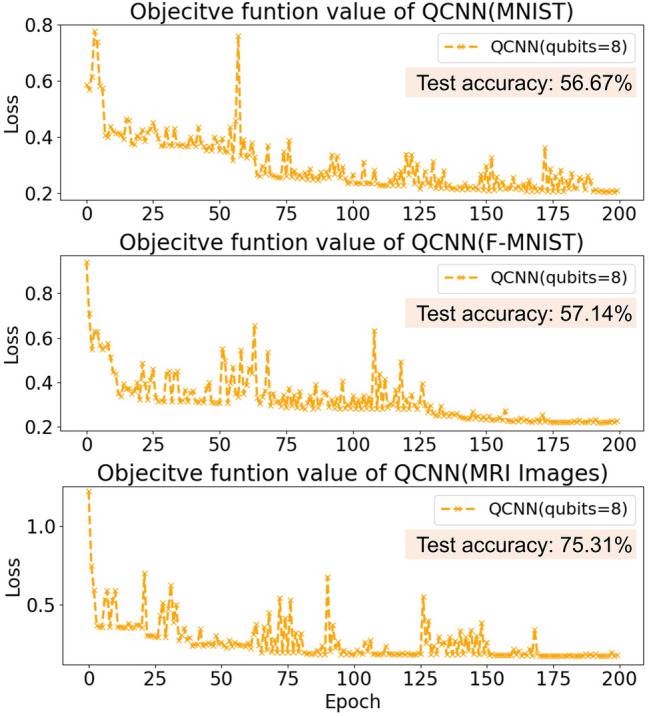
Training loss curves over 200 epochs for different datasets with QCNN.

Hybrid quantum-classical convolutional neural networks (QCCNNs)

To overcome the scalability issues, training instability, and hardware constraints observed in fully QCNNs, hybrid quantum-classical convolutional neural networks (QCCNNs) have been proposed as an extended framework. Unlike QCNNs, which rely entirely on quantum operations for both feature extraction and pooling, QCCNNs replace part of the quantum processing pipeline with classical convolutional layers, while retaining VQCs as local quantum filters. This hybrid approach reduces quantum resource requirements, improves training stability, and enhances compatibility with NISQ devices. In this architecture, quantum convolutional layers apply parametrized quantum gates to locally encoded input data, and classical pooling and fully connected layers follow to complete the learning pipeline. The QCCNN design has been explored in several studies, including the pioneering work of Henderson et al.²², which introduces an encoding-decoding scheme to align quantum outputs with classical operations. More recently, Liu et al.²⁴ further formalized the framework by using VQCs composed of alternating single-qubit rotations and two-qubit entangling gates, including controlled-Z or CNOT, to capture local correlations within data patches. In the quantum convolutional layer, each local region of the input data , such as an image patch, is first mapped into a quantum state through a chosen encoding scheme. Several encoding strategies can be adopted, including angle encoding and threshold encoding, where classical values are mapped onto the parameters of quantum gates. The encoding process can be formally represented as:

6

where denotes the encoding operation and is the initial quantum state of n qubits. Following the encoding, a parametrized quantum circuit acts as the quantum filter:

7

For QCCNNs, we denote the fixed quantum parameters as , which are randomly initialized and remain unchanged during training. This non-trainable design reduces optimization overhead but limits model adaptability and quantum expressiveness. The proposed circuit architecture enables local feature extraction by exploiting quantum entanglement. The output features are obtained by measuring observables on the resulting quantum state, for a measurement operator at location i is defined as:

8

where is selected as the Pauli-Z observable (measured after the circuit), this choice ensures consistency with the based rotations used in the quantum convolutional filter and provides an efficient measurement scheme for feature extraction. Compared with conventional CNN layers, which aggregate features by spatially summing activations across neighboring positions, QCCNNs apply quantum measurements directly to select qubits following local quantum operations. These measurement outcomes capture localized feature information without explicit summation operations. The extracted quantum feature maps are subsequently fed into classical pooling layers for dimensionality reduction and then into fully connected layers to complete the final classification task. While QCCNNs similarly do not yet demonstrate exponential computational advantages, they offer a more hardware adaptive design by leveraging shallow quantum circuits alongside classical processing modules. This hybrid formulation enables more stable training and reduced quantum resource consumption, making it a practical candidate for near-term quantum applications where fully quantum architectures remain infeasible. While prior studies have explored trainable quantum filters, we opt to fix the filter structure following the original Quanvolutional approach. This decision aims to isolate the contribution of the variational quantum classifier, reduce optimization overhead, and ensure reproducibility. Exploring trainable quantum filters remains a promising direction for future work.

Hybrid quantum-classical-quantum convolutional neural network (QCQ-CNN)

While QCCNNs alleviate some of the limitations of fully quantum convolutional neural networks by combining quantum feature extraction with classical layers, their performance remains restricted by the expressiveness of shallow variational circuits and the scalability of quantum encoding schemes. Motivated by recent insights into quantum neural networks, we extend the QCCNN architecture to further exploit the strength of quantum modeling. Zhang et al.³⁰ investigated the trainability of QNNs and demonstrated that step-controlled ansatze can avoid barren plateaus and deliver better convergence and accuracy for binary classification. Beer et al.¹⁶ demonstrate that QNNs exhibit remarkable generalization performance and robustness against noisy training data, reinforcing their suitability for complex learning tasks under realistic conditions. In addition, Abbas et al.¹⁵ show that QNNs can achieve higher expressive capacity than classical neural networks, particularly when designed with structure parameterizations. These observations suggest that QNNs, when carefully constructed, can serve as powerful classifiers.

Inspired by recent advances, we propose a Quantum-Classical-Quantum Convolutional Neural Network (QCQ-CNN). As shown in Fig. 3, the architecture comprises three sequential components: a quantum filter for initial feature extraction, a classical convolutional network for intermediate representation learning, and a quantum neural network (QNN) as the final classification module.

Fig. 3.

The hybrid quantum-classical-quantum convolutional neural network (QCQ-CNN) model. It consists of a quantum filter for patchwise feature extraction, a classical CNN module for learning, and a QNN classifier that uses a ZZFeatureMap and RealAmplitudes ansatz. This hybrid design combines quantum and classical strengths to improve classification. The example shown processes MNIST digit images.

The overall QCQ-CNN pipeline extends the QCCNN framework by adding a downstream quantum neural network classifier and follows a quantum–classical–quantum structure. The front-end quantum filter adopts the quanvolutional layer design proposed by Henderson et al.²², which is functionally similar to the quantum convolutional layer introduced by Liu et al.²⁴. Each image patch is encoded into a quantum state and processed via a shallow variational circuit. Expectation values of Pauli-Z measurements are extracted as nonlinear quantum features, this approach avoids the need for classical nonlinearities such as ReLU. Therefore, the extracted quantum feature maps are subsequently passed to a shallow classical CNN consisting of convolutional, pooling, and fully connected layers. These classical components are computationally efficient, stable, and contribute additional nonlinearities to the hybrid system. The compact representation after flattening and projection, and re-encoded into a quantum state and input into a QNN classifier composed of structured ansatze, including ZZFeatureMap (Fig. 1) and RealAmplitudes (Fig. 4). Since the QNN operates on low-dimensional features, only a small number of qubits are required, significantly reducing resource costs. This design is particularly well suited for current NISQ devices, where limitations in qubit count and coherence time constrain model complexity. Furthermore, the parameterized gates in the RealAmplitudes layer serve as learnable weights, allowing the QNN to perform forward propagation analogous to classical networks via quantum evolution and observable-based measurements. In addition, the depth of the RealAmplitudes ansatz can be systematically increased by repeating its building blocks (e.g., RY–CNOT), enabling us to investigate how the number of quantum parameters affects training dynamics and model expressiveness. Such depth-controlled studies are essential for understanding trade-offs between quantum circuit complexity and performance, especially in the context of barren plateaus and NISQ constraints^32,44.

Fig. 4.

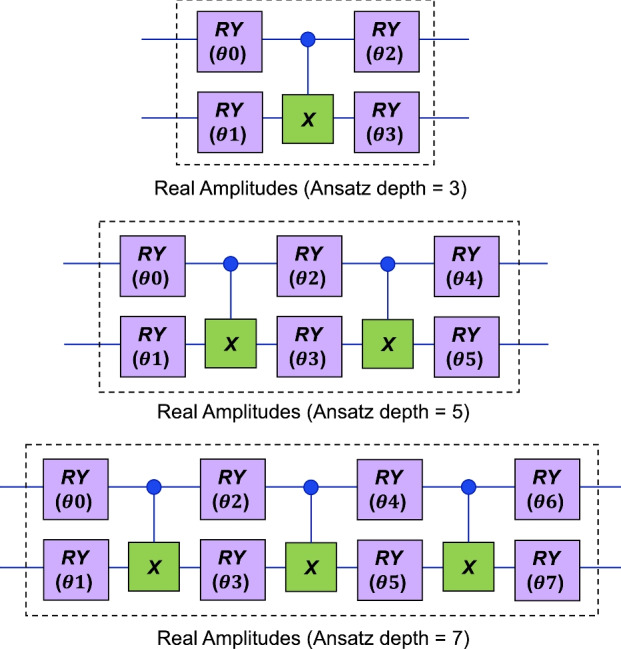
Quantum circuits for real amplitudes with 3, 5, 7 circuit depths, corresponding to 4, 6, and 8 trainable RY parameters, respectively.

Quantum filter feature extraction

To enhance compatibility with noisy intermediate-scale quantum devices, quantum convolutional filters operate on low-dimensional quantum states derived from classical image data. At each position, a local region is extracted from the input image and reshaped into a classical vector , where N denotes the number of qubits used in the quantum filter. This vector is then mapped to a quantum state using a rotational encoding strategy:

9

where each normalized pixel value is encoded as a rotation angle on the Bloch sphere, covering the subspace. The encoded state is subsequently processed by a variational quantum circuit , which consists of L layers of parameterized single-qubit RZ and RY rotations, along with nearest-neighbor CNOT entangling operations:

10

where and are randomly initialized fixed angles and remain unchanged during training. The resulting quantum state becomes:

11

Pauli-Z expectation values are then measured on each qubit to generate classical feature outputs:

12

where values are aggregated to form a multi-channel quantum feature map. For a single-layer 4-qubit circuit, this results in four channels per image, visualized as stacked feature maps in Fig. 3. Notably, in our implementation, the parameters of the quantum filter are randomly initialized and remain fixed during training. This design decouples the expressive yet noisy quantum encoding from the learning stage, reducing training overhead and improving robustness on NISQ devices. Such a fixed-filter strategy allows the quantum module to serve as a non-trainable feature extractor, offering structured quantum representations without incurring the cost or instability of end-to-end quantum optimization.

This choice is motivated by both practical considerations and alignment with established conventions. Specifically, we follow the original QNN architecture²², which employs randomly initialized yet fixed quantum filters. Adopting the same configuration ensures a fair comparison with QCCNN and allows us to isolate the contribution of the downstream variational quantum classifier (VQC). Furthermore, recent studies⁴⁵ have observed that quantum filter parameters tend to exhibit negligible updates during gradient-based training, implying limited benefit from making them trainable. Fixing the quantum filter thus simplifies the optimization landscape, improves convergence stability, and facilitates reproducibility across different simulation platforms.

Classical convolutional processing

These quantum values are stacked across the image to form multi-channel feature maps, which are then passed to a classical CNN module for spatial representation learning:

13

where denotes the trainable weights and biases of the CNN block. As illustrated in Fig. 3, this classical module consists of two convolutional layers (Conv1, Conv2), each followed by a max-pooling operation (Pool1, Pool2) to reduce spatial dimensions and increase feature robustness. The functional composition of this pipeline can be written explicitly as:

14

where each function denotes a specific transformation layer applied to the quantum input in sequence. This convolution–pooling pipeline enables the model to hierarchically abstract mid-level spatial features from the quantum inputs. After the final pooling layer, the resulting tensor is flattened and passed through a fully connected layer, producing a compact latent vector , which serves as the input to the downstream QNN classifier. Beyond providing spatial abstraction, the CNN block substantially contributes to the performance of the hybrid architecture. It introduces a rich set of classical trainable parameters, enabling gradient-based optimization to propagate effectively across the network. Prior works^1,5 have highlighted that embedding classical components between quantum modules improves model stability and convergence in NISQ settings. By absorbing low to mid-level variability, the classical CNN also mitigates the risk of barren plateaus in the variational QNN classifier, allowing quantum resources to focus on learning high-level, expressive decision boundaries.

Quantum neural network classifier

After classical convolutional processing, the compact latent vector obtained by flattening and dense projection is re-encoded into a quantum state and fed into a quantum neural network classifier. Similar to classical neural networks, the QNN performs forward propagation through parameterized quantum evolution and observable measurements. Specifically, a two-qubit quantum feature map inspired by the ZZFeatureMap applies:

15

where denotes an encoding operation composed of local phase rotations and entangling interactions:

16

which embeds both individual features and pairwise correlations directly into the quantum phase. This encoded state is then processed by a variational quantum circuit , constructed using the RealAmplitudes ansatz:

17

where is the circuit depth, and represents all trainable parameters. The and denote the trainable rotation angles applied to the i-th qubit in the l-th ansatz block via RY and RZ gates, respectively. This ansatz alternates parameterized single-qubit rotation layers with fixed entangling CNOT layers and is repeated times to control the expressive capacity of the variational quantum circuit (VQC). In quantum computing, the circuit depth refers to the number of gate layers applied sequentially on the quantum register, the number of time steps required, assuming gates acting on disjoint sets of qubits can be executed in parallel. For variational circuits, the depth corresponds to the number of repeated entangle rotation blocks. Each block contains parameterized gates on every qubit followed by a CNOT entangling layer. For a two-qubit circuit, each repetition introduces two trainable parameters (one per qubit per RY gate), and the entangling layer introduces logical connectivity via . Thus, circuit depths correspond to variational circuits with 4, 6, and 8 trainable parameters in the RY gates respectively. As shown in Fig. 4, each depth level includes repeated blocks of single-qubit rotations followed by entangling CNOT layers (denoted by the green symbols). The number of trainable parameters scales linearly with depth, while entangling layers remain fixed to preserve interpretability and control circuit complexity.

Deeper circuits increase expressive power by enabling more complex unitary transformations. At the same time, they exacerbate the barren plateau phenomenon, characterized by regions of exponentially vanishing gradients in the loss landscape, which significantly impedes optimization³². In our implementation, a depth of achieves an optimal balance between expressivity and trainability, yielding stable convergence and strong performance across datasets. The output quantum state becomes:

18

We extract the final scalar prediction by measuring the expectation value of a Hermitian observable , typically chosen as the Pauli-Z operator acting on the first qubit:

19

and convert this continuous value into a binary prediction via thresholding with a trainable bias term :

20

where is updated during training. This final quantum module allows expressive nonlinear decision boundaries to be modeled at reduced qubit cost, making it well-suited for NISQ-era deployment. The complete training procedure of the proposed QCQ-CNN framework is summarized in Fig. 5.

Fig. 5.

Pseudocode for the training procedure of the QCQ-CNN framework.

Positioning the QNN classifier after the CNN confers three major advantages essential for practical deployment in the NISQ era: (i) The classical convolutional backbone effectively performs dimensionality reduction and spatial abstraction, reducing the number of qubits required in the quantum stage while mitigating cumulative quantum noise. (ii) The expressive capacity of the quantum model is concentrated at the decision boundary, which enhances nonlinear separability without burdening the quantum encoder with low-level feature extraction. (iii) The hybrid architecture benefits from classical optimization stability and quantum nonlinearity, promoting efficient gradient propagation and reducing the risk of barren plateaus. These design choices are theoretically grounded in prior studies^5,38, which demonstrate that shallow qubit variational classifiers can match or outperform classical models when operating on structured, low-dimensional features. Building on this principle, our QCQ-CNN architecture employs the QNN not as a feature generator but as a binary quantum decision module, yielding improvements in both predictive performance and robustness. To substantiate these benefits, we conduct extensive simulations on MNIST, Fashion-MNIST, and an MRI brain tumor dataset. Ablation studies on circuit depth show that increasing the number of ansatz layers enhances model expressiveness, but may introduce convergence instability and noise sensitivity. Empirically, a moderate depth (e.g., a 5-layer RealAmplitudes circuit with 6 trainable RY gates) achieves the best trade-off between accuracy and training stability across datasets. Furthermore, the output from the QNN is derived from the expectation value of a Hermitian observable (e.g., Pauli-Z). This provides a physically grounded and interpretable decision score, offering a distinctive advantage over purely classical classifiers⁴⁶. This observable-based prediction mechanism facilitates model introspection and aligns with recent efforts in explainable quantum learning. In addition, the QCQ-CNN architecture exhibits superior generalization, particularly in limited data or noisy regimes, highlighting its robustness and suitability for practical quantum-classical applications. The following section provides a detailed quantitative evaluation to support these findings.

Numerical simulations and results

To validate the effectiveness and generalizability of our proposed QCQ-CNN architecture, we conduct extensive numerical simulations on a variety of image classification tasks. Our evaluation consists of two main parts: (i) a comparative study across five different models to assess the benefit of quantum components under equal capacity constraints, and (ii) an ablation analysis of the QNN classifier to examine how the ansatz circuit depth influences performance.

Dataset and preprocessing

To evaluate the generalization ability and learning behavior of the proposed QCQ-CNN model, we perform binary classification on three datasets: MNIST, Fashion-MNIST (F-MNIST), and a brain MRI tumor dataset. For MNIST, three binary tasks are constructed using digit pairs (3 vs. 5). F-MNIST is similarly used to construct a binary classification task (T-shirt vs. Trouser). The MRI dataset contains pre-labeled images for brain tumors and nontumor cases. The MNIST and Fashion-MNIST datasets are obtained from the standard TensorFlow/Keras library and used to construct binary classification tasks by selecting specific class pairs. In the revised experimental setup, each task uses a total of 7250 images, consisting of 5000 for training, 1250 for validation, and 1000 for testing. Specifically, for both MNIST and Fashion-MNIST, the training set contains 3125 images from each class, from which 20% are held out to form a balanced validation set. The test set includes 500 images per class. This configuration ensures a more statistically robust evaluation while enabling early stopping and fair comparisons across models. To evaluate the adaptability of the model to practical data scenarios, we additionally include a brain MRI tumor classification task using a publicly available dataset from Kaggle⁴⁷. The original MRI dataset consists of four categories: glioma, meningioma, pituitary tumors, and no tumor. For consistency with binary classification tasks, we group the samples into two classes: benign tumors (790 images) and malignant tumors (2745 images). The dataset is then split into 2089 training images, 653 validation images, and 523 test images.

Comparative model design

We evaluate five different models to analyze the contribution of quantum components at different stages of the hybrid architecture:

• MLP (flatten +dense layer): A purely classical baseline with no quantum components. It directly flattens the grayscale image and applies a fully connected layer with 10 softmax outputs. This model serves as the simplest baseline to highlight the effect of quantum feature learning.

• Quantum filter + MLP (Quanvo + MLP): This model applies the quantum filter, and uses a flatten and dense output layer (MLP) for classification. The quantum feature map generated by the quantum filter is directly flattened and fed into the MLP. It represents a minimal hybrid model with quantum feature extraction only.

• Classical CNN: To ensure a fair comparison, we design a shallow classical CNN with two convolutional layers using 16 and 32 filters ( kernel size), each followed by max-pooling and a final dense output layer. The number of trainable parameters is deliberately limited to maintain parity with the quantum-enhanced models, allowing us to assess whether quantum modules provide benefits under constrained model capacity.

• QCCNN: This hybrid quantum-classical model integrates a fixed quantum filter for feature extraction, followed by a classical CNN and a fully connected output layer for classification. Compared to the classical CNN baseline, it introduces quantum-enhanced input features; compared to QCQ-CNN, it uses a classical rather than quantum classifier. As a strong and well-performing recent model, it serves as a competitive baseline to isolate the effect of adding a QNN classifier, by comparing with CNN and QCQ-CNN.

• QCQ-CNN (proposed): Our full hybrid model combining quantum convolutional feature extraction and a QNN classifier. The first stage applies a quantum filter with stride 2, implemented using PennyLane’s RandomLayers⁴⁸, producing a quantum feature map. This is followed by a shallow CNN backbone and a two-qubit variational quantum circuit (VQC) classifier built using Qiskit⁴⁹ with a ZZFeatureMap and RealAmplitudes ansatz. The quantum circuit is connected to PyTorch⁵⁰ via TorchConnector, enabling end-to-end hybrid optimization.

All models receive inputs resized to , and the output shape of the quantum convolutional layer is fixed at to ensure consistency across models. This unified design enables a controlled and interpretable comparison. Specifically, the model variants are carefully chosen to isolate the contribution of each architectural element. By comparing models MLP and quantum filter + MLP, we evaluate the effectiveness of quantum feature extraction in capturing high-dimensional, non-linear representations. Similarly, comparing models with and without a QNN classifier allows us to assess whether quantum decision modules offer advantages over classical alternatives in terms of expressiveness and interpretability. The inclusion of a classical CNN baseline further grounds the evaluation, demonstrating whether quantum enhancements provide tangible benefits under equivalent model capacity constraints. These comparisons are critical for validating the contribution of quantum modules under realistic NISQ conditions.

Training details

All models are trained for 100 iterations (epochs) using the Adam optimizer with a learning rate of , and the batch size is set to 4 for classical and QCCNN models. To reduce the simulation overhead in quantum layers, QCQ-CNN uses a batch size of 1 for fine-grained gradient updates in hybrid quantum-classical optimization. To ensure consistency, all models are optimized using the cross-entropy loss, detailed as follows:

21

where represents the output vector of the QCQ-CNN, and r denotes the set of all trainable parameters in the model. is the total number of samples in the dataset, and is a binary indicator of whether the class c is the correct label for the sample i. Where is the predicted probability of the sample i belonging to C , according to the output of the model. And we utilized the Adam optimizer for training our model. For the quantum filter block, the quantum feature extractor is non-trainable, while only the CNN weights and QNN variational parameters are optimized, above models are implemented in Python, using TensorFlow and PennyLane^48,51 for quantum feature generation, and PyTorch⁵⁰ with Qiskit and Tensoflow^49,51 for QNN classification, to ensure reliability, each simulation is repeated on multiple datasets and classification tasks.

Model comparison and analysis

To evaluate the classification performance of our proposed QCQ-CNN model, we conducted comprehensive experiments on three binary classification tasks using MNIST (digits 3 vs. 5), Fashion-MNIST (T-shirt/top vs. Trouser), and MRI brain tumor datasets. All models were trained for a fixed 100 epochs with early stopping based on validation accuracy. To ensure statistical robustness, each experiment was repeated ten times with different random seeds. The final results are reported as the average accuracy with standard deviation across these runs, as summarized in Table 1.

Table 1.

Classification accuracy (%) on three binary classification tasks with standard deviation over than ten runs. Bold values indicate the best performance.

Model	MNIST (digits 3 vs 5)	FMNIST (T-shirt/trouser)	MRI brain tumor (benign/malignant)
MLP	96.56 ± 0.13	98.48 ± 0.11	86.10 ± 0.40
Quanvo + MLP	96.86 ± 0.14	98.58 ± 0.13	89.24 ± 0.85
CNN	98.79 ± 0.13	99.19 ± 0.19	89.43 ± 1.00
QCCNN	98.81 ± 0.25	99.28 ± 0.12	90.06 ± 1.00
QCQ-CNN	98.85 ± 0.25	99.41 ± 0.14	95.18 ± 0.65

As shown in Fig. 6, the accuracy and loss curves for five models on two binary classification tasks from the MNIST dataset. We compare models on the task of classifying digits 3 and 5, which often have similar local structures and are harder to separate. This task is considered more challenging due to the visual similarity and overlapping local features of the two classes. Among all models, the proposed QCQ-CNN (red) consistently achieves the highest accuracy and lowest loss, exhibiting both faster convergence and superior final performance. The performance margin is especially clear after the initial 20 epochs, where QCQ-CNN surpasses all baselines by a noticeable gap. In contrast, models using only MLP (orange) or quantum filter followed by MLP (purple) converge more slowly and to lower accuracy levels, highlighting the necessity of spatial feature extraction. QCCNN (blue), which incorporates quantum convolutional features but uses a classical CNN classifier, performs better than the purely classical CNN (green), confirming the effectiveness of quantum feature encoding. However, the full hybrid architecture of QCQ-CNN provides further gains, suggesting that the VQC-based quantum classifier plays a complementary role in enhancing decision boundaries.

Fig. 6.

Accuracy and loss curves over 100 training epochs on the MNIST 3-vs-5 binary classification task. The red line represents the proposed QCQ-CNN model, which combines quantum feature extraction with a VQC classifier. The blue line represents the QCCNN model, which incorporates a quantum filter and classical CNN layers. The green line indicates a shallow classical CNN, while the orange line corresponds to a purely classical fully connected network (MLP). The purple line shows results from a minimal hybrid model using quantum filtering followed by fully connected layers (Quanvo + MLP). The left panel presents the accuracy trends, and the right panel displays the corresponding loss curves.

As shown in Fig. 7, we extend the evaluation to the Fashion-MNIST dataset using a binary classification task between two visually distinct classes: T-shirt/top and Trouser. Overall trends are similar, with QCQ-CNN again achieving the best performance in both accuracy and loss metrics. While other models converge relatively quickly due to the visual separability of the classes, QCQ-CNN still exhibits more stable optimization and achieves a higher final accuracy plateau. The advantage of QCCNN over the classical CNN remains consistent, indicating that quantum filters are effective in encoding discriminative features even in real-world object recognition tasks. Additionally, the performance difference between QCCNN and QCQ-CNN persists, underscoring the added value of the quantum classifier component. This result demonstrates that the quantum filter effectively extracts discriminative features in the high-dimensional Hilbert space and improves the nonlinear representational capacity of the overall model. As shown in Fig. 8, we further evaluate the models on a practical medical imaging task: classifying MRI brain scans into benign and malignant tumors. This scenario involves complex texture patterns and substantial intra-class variation, making the classification problem more realistic and challenging. In Table 1, the QCQ-CNN model again shows clear superiority, reaching a peak accuracy of with a substantial margin of over QCCNN and $5.75% over the classical CNN. As shown in the Table 1, the proposed QCQ-CNN consistently outperforms the baseline models, including purely classical (MLP, CNN) and hybrid quantum-classical (Quanvo + MLP, QCCNN) architectures. The Simulation results on practical datasets indicate that the integration of quantum features and trainable quantum classifiers enhances performance. In particular, performance gains on the more complex F-MNIST and MRI brain tumor classification tasks indicate that the QNN classifier plays a central role in surpassing QCCNN. This improvement reflects the ability of parameterized quantum decision boundaries to capture nonlinear separability and resolve ambiguity near class boundaries. These findings further support the robustness and practical applicability of QCQ-CNN in practical learning scenarios beyond idealized benchmarks.

Fig. 7.

Accuracy and loss curves over 100 training epochs on the Fashion-MNIST binary classification task (T-shirt/top vs Trouser). The red line represents the proposed QCQ-CNN model, which integrates quantum convolutional filtering and a trainable VQC classifier. The blue line indicates the QCCNN model that combines quantum filtering with a classical CNN. The green line denotes a purely classical CNN baseline. The orange line corresponds to a fully connected (MLP-only) model, and the purple line shows the performance of a minimal hybrid model (Quanvo + MLP), which uses quantum filtering followed by dense layers. The left panel presents the accuracy trends, while the right panel displays the corresponding loss curves over training epochs.

Fig. 8.

Accuracy and loss curves over 100 training epochs on the brain MRI classification task (benign vs malignant tumors). The red line represents the proposed QCQ-CNN model, which integrates quantum convolutional filtering and a variational quantum classifier (VQC). The blue line corresponds to the QCCNN model that combines quantum filtering with a classical CNN. The green line denotes a purely classical CNN baseline, while the orange and purple lines indicate models using only fully connected layers (MLP) and quantum filtering followed by MLP, respectively. The left panel shows model accuracy evolution, and the right panel illustrates the loss convergence behavior. QCQ-CNN demonstrates faster convergence and higher final accuracy, highlighting the benefit of combining quantum feature extraction with trainable quantum classification in complex datasets.

Noise-aware evaluation of QCQ-CNN performance

To assess the robustness and practical feasibility of the proposed QCQ-CNN model under realistic quantum conditions, we conduct a series of noise-aware simulations. These experiments specifically target the inference stage of the QCQ-CNN, which uniquely involves a trainable quantum classifier subject to runtime quantum operations. As a testbed, we choose the MNIST binary classification task distinguishing digits 3 and 5. This subset is widely used in quantum machine learning due to its moderate complexity and well-characterized difficulty, making it ideal for controlled robustness analysis. In these experiments, we simulate the effects of quantum noise and measurement uncertainty using two key approaches:

• To provide a reference point, we include an idealized setting where the model is evaluated using noiseless statevector simulation and infinite-shot measurements. This curve represents the upper bound of achievable performance in the absence of quantum noise and sampling variability.

• Finite sampling shots: Instead of using idealized expectation values, we simulate measurements with 128 and 1024 sampling shots to reflect realistic execution on near-term quantum devices.

• Depolarizing noise models: Noise is applied to all quantum gates in the variational quantum circuit. Specifically, single-qubit gates (e.g., RX, RY, RZ) are modeled with depolarizing error rates of , while two-qubit CNOT gates are perturbed with error rates of . These values are consistent with current estimates of gate fidelity on NISQ hardware.

Simulations are executed using the qiskit.AerSimulator in density matrix mode to accurately capture noise propagation and decoherence. For comparison, an ideal (noise-free and infinite-shot) simulation is also included to establish an upper bound on performance.

As shown in Fig. 9, under 128-shot conditions, the presence of depolarizing noise leads to moderate but controlled degradation in training accuracy during early epochs. The intermediate noise level (γ = 0.01, δ = 0.02) shows less fluctuation and faster stabilization, while the clean 128-shot run closely tracks the ideal performance after initial epochs. The impact is noticeable for the highest noise setting (γ = 0.02, δ = 0.03), where the initial convergence is slower. However, the model still converges stably toward high accuracy, with differences across noise levels narrowing after approximately 5 epochs. Increasing the shot count to 1024, as shown in Fig. 10, significantly improves stability and reduces performance variance, with noisy results approaching the ideal case. Even with the highest noise setting (, ), the model maintains strong classification accuracy above 95% after convergence. These results suggest that QCQ-CNN maintains a reasonable level of robustness under certain realistic noise settings. While these simulations do not fully capture the complexity of actual NISQ hardware, such as crosstalk, calibration drift, and measurement errors, they provide an initial indication that the model may tolerate typical noise levels to some extent. These findings represent a preliminary step toward more comprehensive validation using real quantum devices and support the continued investigation of quantum-enhanced inference strategies in practical scenarios.

Fig. 9.

Effect of sampling shots and depolarizing noise on QCQCNN training accuracy (shots = 128).

Fig. 10.

Effect of sampling shots and depolarizing noise on QCQCNN training accuracy (shots = 1024).

Effect of ansatz depth in QNN classifier

To evaluate how quantum circuit depth affects classification performance and training dynamics, we conduct a series of experiments on small-scale datasets. For the MNIST and Fashion-MNIST tasks, only 100 training images (50 per class) are used. This setting reflects a resource-constrained regime and is intentionally chosen to mitigate the high computational cost of deep quantum circuit simulations, especially when the quantum classifier is repeated multiple times. For example, with a repetition setting of res = 3, the variational quantum circuit reaches a depth of 7, significantly increasing simulation time. Despite the limited data, these tasks are sufficient to observe trends in convergence behavior and depth sensitivity. To validate the model’s generalization ability under realistic conditions, the entire MRI brain tumor dataset (containing 3,265 images) is used for training. By including this large and heterogeneous dataset, we enhance the credibility and practical relevance of the evaluation, particularly in assessing QCQ-CNN’s performance in more complex and clinically meaningful scenarios. To evaluate how quantum circuit depth affects classification performance and training dynamics, we investigate the influence of ansatz layer repetitions in the QNN classifier of QCQ-CNN. Specifically, we vary the depth of the RealAmplitudes ansatz, which directly controls the number of trainable parameters and the expressive capacity of the quantum circuit. These numerical evaluations provide preliminary insights into the effects of circuit depth on convergence, generalization, and computational cost within NISQ-relevant settings. As shown in Fig. 11, we analyze the performance of QCQ-CNN with different ansatz depths on three binary classification tasks: (a) MNIST digits 3 vs. 5, (b) Fashion-MNIST categories T-shirt/top vs. Trouser, and (c) brain MRI images of benign and malignant tumors. The models adopt ansatz depths of 3 (black), 5 (purple), and 7 (blue), corresponding to 4, 6, and 8 trainable parameters respectively, as defined in Fig. 4. In the MNIST task shown in Fig. 11a, the model with ansatz depth 3 converges rapidly in early epochs but shows a premature plateau with suboptimal accuracy. The depth 5 model achieves the highest final accuracy with stable convergence, while the depth 7 model exhibits increased fluctuations after around 40 epochs, likely due to overparameterization, which can amplify gradient instability and sensitivity to quantum noise. This behavior reflects a potential trade-off between expressivity and trainability, with the depth 5 model offering the best balance. In the Fashion-MNIST task (Fig. 11b), all models eventually attain high accuracy, but training dynamics diverge. The depth 3 model converges quickly but exhibits a plateau and slight underfitting. The depth 7 model achieves low loss but suffers from accuracy instability, similar to MNIST. In contrast, the depth 5 model maintains stable convergence and outperforms the others in final classification accuracy, again demonstrating its robustness. In the MRI brain tumor classification task (Fig. 11c), the performance differences among depths are less pronounced. While the depth 3 model shows a slight delay during early training, it eventually reaches comparable performance to the deeper circuits. This suggests that with sufficient training, shallow quantum circuits may still generalize well, even in complex medical imaging tasks.

Fig. 11.

Accuracy and loss curves of QCQ-CNN with different ansatz depths on three binary classification tasks: (a) MNIST digits 3 and 5, (b) Fashion-MNIST categories T-shirt/top and Trouser, and (c) MRI brain tumor images of benign and malignant tumors. In all subfigures, the dotted black line represents QCQ-CNN with ansatz depth 3 (number of trainable parameters = 4), the dotted purple line shows depth 5 (number of trainable parameters = 6), and the dotted blue line corresponds to depth 7 (number of trainable parameters = 8). Insets provide zoomed-in views of convergence dynamics; original axis scales are preserved.

In addition, circuit depth introduces non-negligible computational overhead. On the MNIST 3 vs. 5 task, total training time increases from 364.47 seconds at depth 3 to 438.70 seconds at depth 5 (a  20.4% increase), and further to 525.83 seconds at depth 7 (an approximate 44% increase over depth 3). Despite this increased cost, deeper circuits do not translate into improved convergence or generalization, revealing diminishing returns in quantum expressivity beyond a moderate threshold. Although depths 5 and 7 exhibit similar convergence trends and final accuracy across both datasets, their training efficiency differs significantly. On larger or more complex datasets such as F-MNIST and MRI brain tumor, even a modest increase in circuit depth results in a proportional rise in training time and quantum resource consumption. This is due to the deeper ansatz introducing more layers of parameterized rotation and entanglement gates, which increases circuit evaluation cost and amplifies noise sensitivity under NISQ constraints. Considering the trade-off between performance, convergence stability, and resource overhead, we identify ansatz depth (i.e., ansatz repetition parameter reps=2) as the optimal configuration for the QNN classifier across our image classification benchmarks. These results collectively indicate that while deeper ansatz circuits may reduce training loss, they do not necessarily yield better predictive accuracy. The depth 5 configuration consistently provides optimal performance across both easy and hard tasks, and is therefore adopted as the default setting in subsequent numerical simulations.

Conclusion

In summary, we proposed and evaluated a hybrid quantum-classical-quantum convolutional neural network (QCQ-CNN), which integrates quantum convolutional filters, classical CNN layers, and a trainable quantum neural network (QNN) classifier. By introducing trainable quantum parameters at the output stage, QCQ-CNN aims to enhance the expressiveness of decision boundaries in image classification tasks. This design builds upon previous hybrid architectures such as QCCNN, addressing their limitations by enabling end-to-end learning and improved representational capacity through variational quantum circuits. Our numerical simulation across three datasets, MNIST, Fashion-MNIST, and MRI brain tumor classification, demonstrates that QCQ-CNN achieves competitive performance in terms of accuracy and convergence behavior when compared to both classical and hybrid baselines. We conducted a systematic investigation of the impact of quantum ansatz depth and found that circuits of moderate depth provide a favorable trade-off between model expressivity and training stability. In contrast, deeper circuits tend to exhibit instability and signs of barren plateau effects, which hinder optimization. We also conducted noise-aware simulations incorporating depolarizing noise and finite-shot measurements to assess robustness under realistic quantum execution conditions. Results suggest that QCQ-CNN retains its performance advantage and convergence behavior even in the presence of such quantum noise, providing preliminary evidence for its practical viability on near-term quantum hardware. Nonetheless, this work has several limitations. Our evaluations are still constrained to simulated environments and relatively small-scale circuits, which may not directly generalize to large-scale, high-dimensional tasks. In addition, the computational overhead of hybrid models and the current limitations of quantum simulators restrict our ability to explore more complex architectures or larger datasets. Further research is needed to validate these findings on real quantum hardware, extend the model to multi-class or sequential data, and optimize quantum circuit design under resource constraints.

Overall, QCQ-CNN offers a modular and adaptable framework for integrating quantum learning components into classical deep learning pipelines. While our findings are preliminary, they highlight the potential of trainable quantum circuits in enhancing hybrid models and motivate continued exploration of hybrid quantum-classical learning in the NISQ era.

Author contributions

C.L. conceived and designed this study. T.S., Y.F., and X.Y. provided suggestions for improving the manuscript. C.L. and M.H. analyzed the data and refined the experimental design. C.L., X.Y., and M.H. drafted the manuscript. All authors reviewed the manuscript.

Funding

This work was supported in part by the JSPS KAKENHI Grant Number JP23H03411 and JP22K12144, the JST Grant Number JPMJPF2017.

Data availability

The datasets generated during the current study are available from the corresponding authors on reasonable request. The dataset used for the simulation is available at https://www.kaggle.com/datasets/masoudnickparvar/brain-tumor-mri-dataset.

Code availability

The code used to develop, train, and evaluate the hybrid quantum-classical convolutional neural network (QCQ-CNN) is publicly available at the following GitHub repository: https://github.com/ChrisRyu2101/hybrid_quantum-classical-quantum_cnn/tree/main.

Competing interests

The authors declare no competing interests.

References

- 1.Biamonte, J. et al. Quantum machine learning. Nature549, 195–202 (2017). [DOI] [PubMed] [Google Scholar]
- 2.Huang, H.-Y. et al. Power of data in quantum machine learning. Nat. Commun.12, 2631 (2021). [DOI] [PMC free article] [PubMed] [Google Scholar]
- 3.Bouland, A., Fefferman, B., Nirkhe, C. & Vazirani, U. On the complexity and verification of quantum random circuit sampling. Nat. Phys.15, 159–163 (2019). [Google Scholar]
- 4.Cazorla, C. & Boronat, J. Simulation and understanding of atomic and molecular quantum crystals. Rev. Mod. Phys.89, 035003 (2017). [Google Scholar]
- 5.Benedetti, M., Lloyd, E., Sack, S. & Fiorentini, M. Parameterized quantum circuits as machine learning models. Quantum Sci. Technol.4, 043001 (2019). [Google Scholar]
- 6.Kandala, A. et al. Hardware-efficient variational quantum eigensolver for small molecules and quantum magnets. Nature549, 242–246 (2017). [DOI] [PubMed] [Google Scholar]
- 7.Guerreschi, G. G. & Matsuura, A. Y. Qaoa for max-cut requires hundreds of qubits for quantum speed-up. Sci. Rep.9, 6903 (2019). [DOI] [PMC free article] [PubMed] [Google Scholar]
- 8.Long, C., Futamura, Y., Ye, X. & Sakurai, T. Quantum algorithm for regularized spectral clustering. In Proceedings of the 2023 15th International Conference on Machine Learning and Computing 5–11 (2023).
- 9.Lloyd, S. & Weedbrook, C. Quantum generative adversarial learning. Phys. Rev. Lett.121, 040502 (2018). [DOI] [PubMed] [Google Scholar]
- 10.Chen, S.Y.-C. et al. Variational quantum circuits for deep reinforcement learning. IEEE Access8, 141007–141024 (2020). [Google Scholar]
- 11.O’shea, K. & Nash, R. An introduction to convolutional neural networks. arXiv preprintarXiv:1511.08458 (2015).
- 12.Gu, J. et al. Recent advances in convolutional neural networks. Pattern Recognit.77, 354–377 (2018). [Google Scholar]
- 13.Yamashita, R., Nishio, M., Do, R. K. G. & Togashi, K. Convolutional neural networks: an overview and application in radiology. Insights Imaging9, 611–629 (2018). [DOI] [PMC free article] [PubMed] [Google Scholar]
- 14.Li, Z., Liu, F., Yang, W., Peng, S. & Zhou, J. A survey of convolutional neural networks: analysis, applications, and prospects. IEEE Trans. Neural Netw. Learn. Syst.33, 6999–7019 (2021). [DOI] [PubMed] [Google Scholar]
- 15.Abbas, A. et al. The power of quantum neural networks. Nat. Comput. Sci.1, 403–409 (2021). [DOI] [PubMed] [Google Scholar]
- 16.Beer, K. et al. Training deep quantum neural networks. Nat. Commun.11, 808 (2020). [DOI] [PMC free article] [PubMed] [Google Scholar]
- 17.Cong, I., Choi, S. & Lukin, M. D. Quantum convolutional neural networks. Nat. Phys.15, 1273–1278 (2019). [Google Scholar]
- 18.Vidal, G. Class of quantum many-body states that can be efficiently simulated. Phys. Rev. Lett.101, 110501 (2008). [DOI] [PubMed] [Google Scholar]
- 19.Li, G., Ding, Y. & Xie, Y. Tackling the qubit mapping problem for nisq-era quantum devices. In Proceedings of the Twenty-Fourth International Conference on Architectural Support for Programming Languages and Operating Systems 1001–1014 (2019).
- 20.March, N. H., Young, W. H. & Sampanthar, S. The Many-Body Problem in Quantum Mechanics (Courier Corporation, 1995).
- 21.Wei, S., Chen, Y., Zhou, Z. & Long, G. A quantum convolutional neural network on nisq devices. AAPPS Bull.32, 1–11 (2022). [Google Scholar]
- 22.Henderson, M., Shakya, S., Pradhan, S. & Cook, T. Quanvolutional neural networks: powering image recognition with quantum circuits. Quantum Mach. Intell.2, 2 (2020). [Google Scholar]
- 23.Brandao, F. G., Harrow, A. W. & Horodecki, M. Local random quantum circuits are approximate polynomial-designs. Commun. Math. Phys.346, 397–434 (2016). [Google Scholar]
- 24.Liu, J. et al. Hybrid quantum-classical convolutional neural networks. Sci. China Phys. Mech. Astron.64, 290311 (2021). [Google Scholar]
- 25.Fan, F., Shi, Y., Guggemos, T. & Zhu, X. X. Hybrid quantum-classical convolutional neural network model for image classification. IEEE Trans. Neural Netw. Learn. Syst., 1–15. 10.1109/TNNLS.2023.3312170 (2023). [DOI] [PubMed]
- 26.Hur, T., Kim, L. & Park, D. K. Quantum convolutional neural network for classical data classification. Quantum Mach. Intell.4, 3 (2022). [Google Scholar]
- 27.Gottesman, D. An introduction to quantum error correction and fault-tolerant quantum computation. In Quantum Information Science and Its Contributions to Mathematics, Proceedings of Symposia in Applied Mathematics, Vol. 68, 13–58 (2010).
- 28.Cross, A. W., Bishop, L. S., Sheldon, S., Nation, P. D. & Gambetta, J. M. Validating quantum computers using randomized model circuits. Phys. Rev. A100, 032328 (2019). [Google Scholar]
- 29.Zaman, F. et al. Comparative analysis of hybrid quantum-classical models for image classification. Mathematics11, 328. 10.3390/math11020328 (2023). [Google Scholar]
- 30.Zhang, K., Hsieh, M.-H., Liu, L. & Tao, D. Toward trainability of quantum neural networks. arXiv preprintarXiv:2011.06258 (2020).
- 31.Sim, S., Johnson, P. D. & Aspuru-Guzik, A. Expressibility and entangling capability of parameterized quantum circuits for hybrid quantum-classical algorithms. Adv. Quantum Technol.2, 1900070. 10.1002/qute.201900070 (2019). [Google Scholar]
- 32.McClean, J. R., Boixo, S., Smelyanskiy, V. N., Babbush, R. & Neven, H. Barren plateaus in quantum neural network training landscapes. Nat. Commun.9, 4812. 10.1038/s41467-018-07090-4 (2018). [DOI] [PMC free article] [PubMed] [Google Scholar]
- 33.Ramezani, S. B., Sommers, A., Manchukonda, H. K., Rahimi, S. & Amirlatifi, A. Machine learning algorithms in quantum computing: A survey. In 2020 International joint conference on neural networks (IJCNN), 1–8 (IEEE, 2020).
- 34.Nielsen, M. A. & Chuang, I. L. Quantum Computation and Quantum Information (Cambridge University Press, 2010).
- 35.Dallaire-Demers, P.-L., Romero, J., Veis, L., Sim, S. & Aspuru-Guzik, A. Low-depth circuit ansatz for preparing correlated fermionic states on a quantum computer. Quantum Sci. Technol.4, 045005 (2019). [Google Scholar]
- 36.Zhou, Z., Du, Y., Tian, X. & Tao, D. Qaoa-in-qaoa: Solving large-scale maxcut problems on small quantum machines. Phys. Rev. Appl.19, 024027 (2023). [Google Scholar]
- 37.Kao, P.-Y. et al. Exploring the advantages of quantum generative adversarial networks in generative chemistry. J. Chem. Inf. Model.63, 3307–3318 (2023). [DOI] [PMC free article] [PubMed] [Google Scholar]
- 38.Schuld, M., Bocharov, A., Svore, K. M. & Wiebe, N. Circuit-centric quantum classifiers. Phys. Rev. A101, 032308. 10.1103/PhysRevA.101.032308 (2020). [Google Scholar]
- 39.Mari, A., Bromley, T. R., Izaac, J., Schuld, M. & Killoran, N. Transfer learning in hybrid classical-quantum neural networks. Quantum4, 340 (2020). [Google Scholar]
- 40.Schuld, M., Bocharov, A., Svore, K. M. & Wiebe, N. Effect of data encoding on the expressive power of variational quantum-machine-learning models. PRX Quantum2, 040348 (2021). [Google Scholar]
- 41.Voulodimos, A., Doulamis, N., Doulamis, A. & Protopapadakis, E. Deep learning for computer vision: A brief review. Comput. Intell. Neurosci.2018 (2018). [DOI] [PMC free article] [PubMed]
- 42.Yarotsky, D. Error bounds for approximations with deep relu networks. Neural Netw.94, 103–114 (2017). [DOI] [PubMed] [Google Scholar]
- 43.Ruby, U. & Yendapalli, V. Binary cross entropy with deep learning technique for image classification. Int. J. Adv. Trends Comput. Sci. Eng.9 (2020).
- 44.Cerezo, M., Sone, A., Volkoff, T., Cincio, L. & Coles, P. J. Cost function dependent barren plateaus in shallow parametrized quantum circuits. Nat. Commun.12, 1791. 10.1038/s41467-021-21728-w (2021). [DOI] [PMC free article] [PubMed] [Google Scholar]
- 45.Ceschini, A. et al. On hybrid quanvolutional neural networks optimization. Quantum Mach. Intell.7, 18. 10.1007/s42484-025-00241-z (2025). [Google Scholar]
- 46.Schuld, M. & Petruccione, F. Machine Learning with Quantum Computers (Springer, 2021).
- 47.Nickparvar, M. Brain tumor mri dataset (2020). https://www.kaggle.com/datasets/masoudnickparvar/brain-tumor-mri-dataset. Accessed: 2024-05-01.
- 48.Bergholm, V. et al. Pennylane: Automatic differentiation of hybrid quantum-classical computations. arXiv preprintarXiv:1811.04968 (2018).
- 49.Cross, A. The ibm q experience and qiskit open-source quantum computing software. In APS March Meeting Abstracts, Vol. 2018, L58-003 (2018). [Google Scholar]
- 50.Paszke, A. et al. Automatic differentiation in pytorch. Placeholder J. (2017).
- 51.Pang, B., Nijkamp, E. & Wu, Y. N. Deep learning with tensorflow: A review. J. Educ. Behav. Stat.45, 227–248 (2020). [Google Scholar]
Associated Data
This section collects any data citations, data availability statements, or supplementary materials included in this article.
Data Availability Statement