AI-driven multi-omics modeling of myalgic encephalomyelitis/chronic fatigue syndrome

Abstract

Myalgic encephalomyelitis/chronic fatigue syndrome (ME/CFS) is a chronic illness with a multifactorial etiology and heterogeneous symptomatology, posing major challenges for diagnosis and treatment. Here we present BioMapAI, a supervised deep neural network trained on a 4-year, longitudinal, multi-omics dataset from 249 participants, which integrates gut metagenomics, plasma metabolomics, immune cell profiling, blood laboratory data and detailed clinical symptoms. By simultaneously modeling these diverse data types to predict clinical severity, BioMapAI identifies disease- and symptom-specific biomarkers and classifies ME/CFS in both held-out and independent external cohorts. Using an explainable AI approach, we construct a unique connectivity map spanning the microbiome, immune system and plasma metabolome in health and ME/CFS adjusted for age, gender and additional clinical factors. This map uncovers altered associations between microbial metabolism (for example, short-chain fatty acids, branched-chain amino acids, tryptophan, benzoate), plasma lipids and bile acids, and heightened inflammatory responses in mucosal and inflammatory T cell subsets (MAIT, γδT) secreting IFN-γ and GzA. Overall, BioMapAI provides unprecedented systems-level insights into ME/CFS, refining existing hypotheses and hypothesizing unique mechanisms—specifically, how multi-omics dynamics are associated to the disease’s heterogeneous symptoms.

Myalgic encephalomyelitis/chronic fatigue syndrome (ME/CFS) is a debilitating, multisystem illness that often persists for years or even decades and presents with substantial heterogeneity in clinical manifestations. Affecting more than 10 million individuals worldwide, ME/CFS is characterized by persistent fatigue, post-exertional malaise, multi-site pain, sleep disturbances, orthostatic intolerance, cognitive impairment, gastrointestinal symptoms and other issues. This complexity not only hinders timely diagnosis but also poses notable challenges for effective treatment. The pathogenesis of ME/CFS is not well understood, with some triggers believed to include viral infections such as Epstein-Barr virus (EBV)¹, enteroviruses² and SARS coronavirus³, in addition to bacterial infections and other causes⁴. As a chronic disease, ME/CFS can persist for years or often a lifetime, with each patient developing distinct illness patterns⁵. Hence, a single standardized approach to clinical care and symptom management is unlikely to suffice; instead, personalized, symptom-specific strategies may be necessary to effectively address the multifaceted nature of ME/CFS.

For ME/CFS and other chronic diseases such as cancer, diabetes, rheumatoid arthritis (RA) and long COVID, this heterogeneity has been problematic to accommodate in research studies, leaving substantial knowledge and technical gaps⁶. The approach of most cohort studies is to focus on identifying one or two key disease indicators, such as HbA1C levels for diabetes or survival rates for cancer, even with the advent of multi-omics. This approach has difficulty accommodating the highly multifactorial etiology and progression of most chronic diseases, with different patients exhibiting varying symptoms and disease markers⁷. To address this challenge, methods must link a more complex matrix of disease-associated outcomes with a range of omics data types to enable precise targeting of biomarkers tailored to each patient’s specific symptoms.

In this study, we generated and assembled a longitudinal, multi-omics dataset from 153 patients with ME/CFS and 96 age- and gender-matched healthy controls, encompassing gut metagenomics, plasma metabolomics, immune cell profiling (including activation and cytokine measures), blood labs, detailed clinical symptoms and lifestyle surveys. To integrate these diverse data types with ME/CFS symptomatology, we developed BioMapAI, an explainable supervised deep neural network (DNN) that maps multi-omics profiles to a matrix of clinical symptoms. We aimed to identify disease biomarkers for ME/CFS, including those specifically tied to its heterogeneous symptomatology, and map interactions among the microbiome, immune system and metabolome rather than focusing on single or pairwise data types.

Using BioMapAI, we identified both disease- and symptom-specific biomarkers, reconstructed key clinical symptoms and classified ME/CFS disease in held-out and external cohorts. We then constructed a comprehensive multi-omics connectivity map that refines existing hypotheses and proposes unique ones regarding microbial, metabolomic and immune factors in ME/CFS. Critically, we accounted for confounders such as age and gender to contextualize the interplay among data types in health versus disease. For example, we observed that depletion of microbial short-chain fatty acids (for example, butyrate) and branched-chain amino acids (BCAAs) in ME/CFS is linked to abnormal activation of mucosal and inflammatory immune cells (MAIT and γδT), which produce IFN-γ and GzA—an altered dynamic correlated with worse perceived health and reduced social activity. Furthermore, microbial metabolites such as tryptophan and benzoate displayed fewer connections with plasma lipids in patients, an association that in turn tracked with fatigue, emotional dysregulation and sleep disturbances.

This dataset is among the most comprehensive multi-omics resources assembled for ME/CFS (including other complex chronic diseases). We further introduce an innovative AI approach that begins to address the multifaceted nature of this chronic disease, generating unique hypotheses for host–microbiome interactions in both health and ME/CFS. Given the recognized parallels in both etiology and clinical presentation between ME/CFS and long COVID^8,9, studying ME/CFS can offer broader insights into the pathophysiology of postviral syndromes. More generally, our AI-driven framework may prove valuable for other complex conditions where symptom variability cannot be fully captured by a single data type.

Results

Cohort overview

We tracked 249 participants over 3 to 4 years, including 153 patients with ME/CFS (75 ‘short-term’ with disease symptoms <4 years and 78 ‘long-term’ with disease symptoms >10 years) and 96 healthy controls (Fig. 1a and Supplementary Table 1). The cohort is 68% female and 32% male, aligning with the epidemiological data showing that women are three to four times more likely to develop ME/CFS^10,11. Participants ranged in age from 19 to 68 y, with body mass indexes (BMIs) from 16 to 43 kg/m². Throughout the study, we collected detailed clinical metadata, blood samples and fecal samples. In total, 1471 biological samples were collected across all participants at 515 time points (Methods, Extended Data Fig. 1a and Supplementary Table 1).

Fig. 1 ∣. Cohort summary and heterogeneity of ME/CFS.

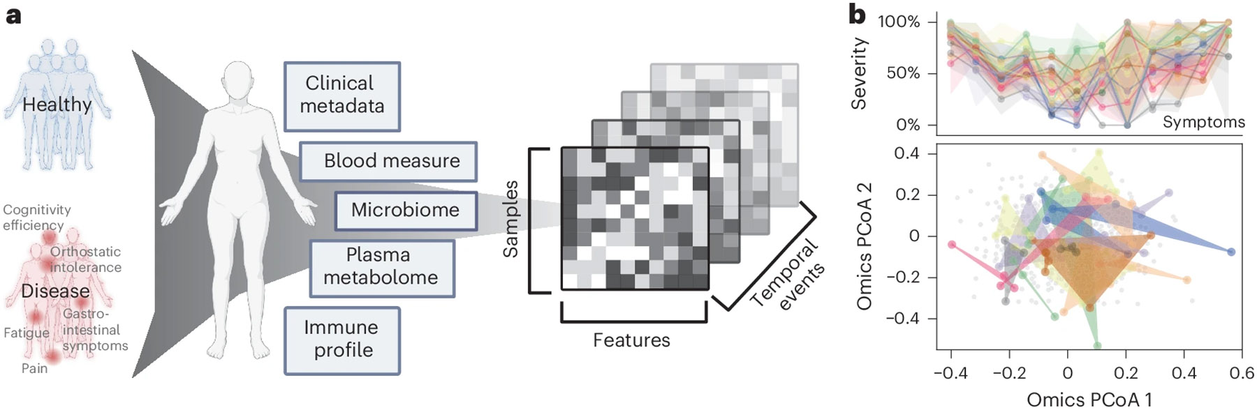
a, Cohort design and omics profiling. 96 healthy donors and 153 patients with ME/CFS were followed over 3 to 4 years with yearly sampling. Clinical metadata including lifestyle and dietary surveys, blood clinical laboratory measures ($n=503$), gut microbiome ($n=479$), plasma metabolome ($n=414$) and immune profiles ($n=489$) were collected (Supplementary Table 1 and Extended Data Fig. 1a). Created in BioRender. Xiong, R. (2025) https://BioRender.com/adqusn8. b, Heterogeneity and nonlinear progression of ME/CFS in symptom severity and omics profiles. This section highlights variability in symptom severity (top) and omics profiles (bottom) for 20 representative patients with ME/CFS over three to four time points. Top: symptom severity is shown for 12 major clinical symptoms ($x$ axis, with each column representing one symptom) against severity scores (scaled from 0% (no symptom) to 100% (most severe), $y$ axis) for each patient (each represented by a distinct color). Lines indicate average severity, and shaded areas represent the severity range across time points (controls shown in Extended Data Fig. 1b). For ME/CFS symptomatology, b (top) highlights substantial heterogeneity over time, as shown by the widespread shaded areas. Extended Data Fig. 1f,g further confirms the absence of consistent temporal patterns, with symptom severity fluctuating considerably over time. Notably, among the 12 symptoms, trends differed: fatigue (symptom 1) remains consistently severe over years, whereas emotional dysregulation (symptom 8) exhibits notable variability and instability over time (Extended Data Fig. 1g). Bottom: PCoA of integrated omics data. The background gray dots represent the entire cohort, defining the overall range of variation in the PCoA space. Colored dots highlight omics-level heterogeneity, with each set of same-colored dots corresponding to an individual’s different time points. The spread and overlap of the colored space reflect the diversity in omics signatures of patients versus the more consistent pattern typical of controls (Extended Data Fig. 1c).

Blood samples were sent for clinical testing at Quest Laboratory (48 features measured, $n=503$ samples) and fractionated into peripheral blood mononuclear cells (PBMCs) (which were examined via flow cytometry, yielding data on 443 immune cells and cytokines ($n=489$), plasma and serum (for untargeted liquid chromatography with tandem mass spectrometry, identifying 958 metabolites ($n=414$)). Detailed demographic documentation and questionnaires covering medication use, medical history and key ME/CFS symptoms were collected (Methods). Finally, whole-genome shotgun metagenomic sequencing of stool samples ($n=479$) produced an average of 12,302,079 high-quality, classifiable reads per sample, detailing gut microbiome composition (1,293 species detected) and KEGG gene function (9,993 genes reconstructed).

Heterogeneity and nonlinear progression of ME/CFS

First, we demonstrated the phenotypic complexity and heterogeneity of ME/CFS. Collaborating with clinical experts, we consolidated detailed questionnaires and clinical metadata foundational to diagnosing ME/CFS into 12 essential clinical scores (Methods). These scores covered core symptoms including physical and mental health, fatigue, pain levels, cognitive efficiency, sleep disturbances, orthostatic intolerance and gastrointestinal issues (Supplementary Table 1).

Although healthy individuals consistently presented low symptom scores (Extended Data Fig. 1d,f), patients with ME/CFS exhibited significant variability in symptom severity, with each individual showing different predominant symptoms (Fig. 1b and Extended Data Fig. 1c,g). Principal coordinates analysis (PCoA) of the omics matrices highlighted the difficulty in distinguishing patients from controls, emphasizing the complex symptomatology of ME/CFS and the challenges in developing predictive models (Extended Data Fig. 1e). Additionally, over time, in contrast to the stable patterns typical of healthy individuals (Extended Data Fig. 1b), patients with ME/CFS demonstrated distinctly varied patterns each year, as evidenced by the diversity in symptom severity and noticeable separation on the omics PCoA (Fig. 1b and Extended Data Fig. 1c). Despite using multiple longitudinal models (Methods), we found no consistent temporal signals, confirming the nonlinear progression of ME/CFS.

This individualized, multifaceted and dynamic nature of ME/CFS that intensifies with disease progression necessitates unique approaches that extend beyond simple disease versus control comparisons. Here, we created and implemented an AI-driven model that integrates the multi-omics profiles to learn host phenotypes. This allowed us not only to develop a disease classifier but also, more importantly, to identify specific biomarker sets for each clinical symptom as well as unique interaction networks that differed between patients and controls.

BioMapAI, a neural network connects omic to multi-outcomes

ME/CFS research is hindered by the complexity of its clinical phenotypes and biological measurements, which are highly individualized. To associate multi-omics data with clinical symptoms, a model must accommodate the learning of multiple different outcomes within a single framework. However, traditional machine learning models are generally designed to predict a single categorical outcome or continuous variable^12-14. This simplified disease classification and conventional biomarker identification typically fails to encapsulate the heterogeneity of complex diseases^15,16. Our goal was to integrate multi-omics data with clinical symptoms into a single model, which would enable a direct comparison of the predictive value of different omics datasets and the identification of symptom-specific biomarkers within a unified framework.

We developed an AI-powered multi-omics framework, BioMapAI, a fully connected DNN that inputs omics matrices ($X$), and outputs a mixed-type outcome matrix ($Y$), thereby mapping multiple omics features to multiple clinical indicators (Fig. 2a). By assigning tailored loss functions for each output to each output based on its data type (Methods), BioMapAI aims to comprehensively learn every $y$ (that is, each of the 12 continuous or categorical clinical scores in this study), using the omics data inputs. Between the input layer $X$ and the output layer $Y=[y_1,y_2,\dots ,y_n]$, the model consists of two shared hidden layers ($Z^1$ with 64 nodes, and $Z^2$ with 32 nodes) for general pattern learning, followed by a parallel hidden layer ($Z^3=[z_1^3,z_2^3,\dots ,z_n^3]$), with sublayers ($z_n^3$, each with 8 nodes) tailored for each outcome ($y_n$), to capture outcome-specific patterns (Fig. 2a). This unique architecture (two shared and one specific hidden layer) allows the model to capture both general and output-specific patterns. This model is made explainable by incorporating a SHAP (SHapley Additive exPlanations) explainer, which quantifies the feature importance of each predictions, providing both local (symptom-level) and global (disease-level) interpretability, and flexible by automatically finding appropriate learning goals and loss functions for each type of outcomes (without need of format refinement), facilitating BioMapAI’s potential adaptability to broader research applications.

Fig. 2 ∣. BioMapAI’s model structure and performance.

a, BioMapAI’s structure. BioMapAI is a fully connected DNN composed of an input layer ($X$), a normalization layer, three sequential hidden layers ($Z^1$, $Z^2$, $Z^3$), and one output layer ($Y$). Hidden layer $Z^1$ (64 nodes) and hidden layer $Z^2$ (32 nodes) feature a dropout ratio of 50% to prevent overfitting. Hidden layer 3 has 12 parallel sublayers, each with 8 nodes ($Z^3=[z_1^3,z_2^3,\dots ,z_{12}^3]$) to learn 12 objects in the output layer ($Y=[y^1,y^2,\dots ,y^{12}]$) representing key clinical symptoms of ME/CFS. In total, we used six inputs ($X$): five individual omics and one merged omics integrating the most important features. Created in BioRender. Xiong, R. (2025) https://BioRender.com/v9fnv0r. b, True versus predicted clinical scores highlight BioMapAI’s accuracy. Three example density maps (full set, Extended Data Fig. 2a) compare the true score, $y$ (Column 1) against BioMapAI’s predictions generated from different omics. $y$ axis represents the diversity along the $x$ axis for each omics. Color gradient from blue (lower density) to red (higher density) illustrates the occurrence frequency, with dashed lines indicating key statistical percentiles. c, Omics’ strengths in symptom prediction. Each of the 12 axes represents a clinical score output ($Y=[y_1,y_2,\dots ,y_{12}]$), with five colors denoting the omics datasets used for model training. The spread of each color along an axis reflects the 1 – normalized mean square error (MSE) (Supplementary Table 2) between the actual, $y$, and the predicted, $\widehat{y}$, outputs, illustrating the predictive strength or weakness of each omics for specific clinical scores. The radial scale ranges from 0.8 (center) to 1.0 (outer circle), where values closer to the outer edge correspond to lower MSE and better predictions. d, BioMapAI’s performance in healthy versus disease classification (10-fold cross-validation and held-out data). ROC curves show BioMapAI’s performance in disease classification using each omics dataset separately or combined (‘Omics’), with the AUC in parentheses showing prediction accuracy (full report in Supplementary Table 3). The dashed line represents a baseline for comparison. e, Validation of BioMapAI with external cohorts. External cohorts with microbiome data (Guo¹⁷, Raijmakers¹⁸) and metabolome data (Germain¹⁹, Che²⁰) were used to test BioMapAI’s model, underscoring its prediction accuracy (detailed classification matrix, Supplementary Table 3).

BioMapAI, reconstructing symptoms and classifying disease

BioMapAI is a supervised DL AI framework that connects a biological omics matrix to multiple phenotypic outputs. Here, we trained and validated it on our ME/CFS dataset, using a tenfold cross-validation. Additionally, 10% of the data was held out as an independent validation set, separate from the cross-validation process, to assess the model’s prediction accuracy (Methods and Supplementary Tables 3 and 6). We trained and reported one model per omics dataset (GitHub), collectively named DeepMECFS for the ME/CFS community—for example, DeepMECFS-Immune for the immune matrix and DeepMECFS-Metabolome for the metabolome matrix. Furthermore, we integrated the most predictive features from each omics model into a comprehensive profile of 154 features (Methods), and named the model DeepMECFS-Omics. Those trained models were represented the structure of diverse clinical symptom score types and as anticipated given patient symptomatology, discriminated between healthy individuals and patients (Fig. 2, Extended Data Fig. 2 and Supplementary Tables 2 and 3), for example in physical health and pain scores. Though compressing some inherent variance, BioMapAI reconstructed key statistical measures such as the mean and interquartile range (IQR) (25%–75%), and highlighted the distinctions between healthy and disease (Fig. 2b, Extended Data Fig. 2a,b and Supplementary Table 2).

To determine the accuracy of BioMapAI’s reconstructed clinical scores, we compared their ability to discriminate patients with ME/CFS from controls with the original clinical scores. We used one additional fully connected layer to regress the 12 predicted clinical scores $\widehat{\mathrm{Y}}$ (12, ) into a binary outcome of patient vs. control $\widehat{\mathrm{y}}$(1,). Because the diagnosis of ME/CFS relies on clinical interpretation of key symptoms (that is, the original clinical scores), the original clinical scores have near-perfect accuracy in classification, as expected (area under the curve (AUC) >99%; Extended Data Fig. 2c). BioMapAI’s predicted scores achieved a 91% AUC in distinguishing disease from healthy controls as evaluated through 10-fold cross-validation (Fig. 2d). We also compared it with four machine learning models (a generalized linear model with elastic net regularization (Glmnet), Glmnet with interaction terms, support vector machine (SVM), and gradient boosting) and a deep learning model (DNN) with two fully connected layers but without the third spread-out hidden layer (Supplementary Table 3). In terms of the 10-fold cross-validation for disease classification, BioMapAI, DNN and Glmnet performed comparably overall. BioMapAI showed slightly better performance with the full omics dataset (AUC = 91.5%), immune data (81.8%) and species data (74.5%), whereas Glmnet had a higher AUC in metabolome (79.0%) and blood laboratory (Quest) data (72.5%).

We tested BioMapAI’s ability to classify disease with unseen data, including held-out cohort datasets (Fig. 2d and Supplementary Table 3) and independent, previously published ME/CFS cohorts (Fig. 2e and Supplementary Table 3). In the held-out datasets, BioMapAI had higher AUC in omics (AUC = 82.3%), immune (78.5%), KEGG (69.1%), species (71.5%), and metabolome (76.4%), whereas Glmnet excelled in blood laboratory (Quest) data (74.8%). Public datasets included two microbiome cohorts (Guo et al. (United States)¹⁷ and Raijmakers et al. (Netherlands)¹⁸) and two metabolome cohorts (Germain et al. (United States)¹⁹ and Che et al. (United States)²⁰). Bio-MapAI had a higher AUC than other models in five out of six external comparisons: Guo (species, AUC = 71.9%; KEGG, 59.1%), Raijmakers (KEGG, 60.6%), Germain (metabolome, 68.1%) and Che (metabolome, 61.3%). The DNN model had the highest AUC in Raijmakers, species (77.3%) (Fig. 2e, Supplementary Table 3). BioMapAI’s accuracy using these external datasets was lower reflecting cohort differences and the absence of some input features (for example, metabolomic features only overlapped by 79% and 19% for the two studies, respectively). Despite the challenges of validating traditional microbiome and metabolite ML models using external cohorts (often having technical and clinical differences^21,22), BioMapAI still has better performance at five out of six comparisons. This highlights the value of incorporating clinical symptoms into a classification model, demonstrating that connecting omics features to clinical symptoms improves disease classification.

Omics strengths varied in symptom prediction

One innovation of BioMapAI is its ability to leverage different omics data to predict individual clinical scores in addition to disease vs. healthy classification. We evaluated the predictive accuracy by calculating the mean squared error (MSE) between actual ($y$) and predicted ($\widehat{y}$) scores and observed that the different omics showed varying strengths in predicting clinical scores (Fig. 2c), likely due in part to the wide differences in dimensionality specific to each data type. Immune profiling consistently had the highest ability to forecast a wide range of symptoms, including pain, fatigue, orthostatic intolerance and general health perception, underscoring the immune system’s crucial role in health regulation. In contrast, blood measurements demonstrated limited predictive ability, except for cognitive efficiency, likely owing to their limited focus on 48 specific blood bioactives. Plasma metabolomics, which encompasses nearly a thousand measurements, performed significantly better with notable correlations with facets of physical health and social activity. These findings corroborate published metabolites and mortality^23,24, longevity^25,26, cognitive function²⁷ and social interactions^28-30. Microbiome profiles surpassed other omics in predicting gastrointestinal abnormalities (as anticipated^31,32), emotional well-being and sleep disturbances, supporting recently established links in gut–brain health^33-35.

BioMapAI identified disease- and symptom-specific biomarkers

Deep learning (DL) models are often referred to as ‘black box’, with limited ability to identify and evaluate specific features that influence the model’s predictions. BioMapAI is made explainable by incorporating SHAP values, which quantify how each feature influenced the model’s predictions. BioMapAI’s architecture (two shared layers ($Z^1$ and $Z^2$) for general disease pattern learning and one parallel layer for each clinical score; $Z^3=[z_1^3,z_{2,}^3,\dots ,z_{12}^3]$) allowed us to identify both disease-specific biomarkers, which are shared across symptoms and models (Extended Data Fig. 3 and Supplementary Table 4), and symptom-specific biomarkers, which are tailored to each clinical symptom (Fig. 3, Extended Data Figs. 4 and 5 and Supplementary Table 5).

Fig. 3 ∣. BioMapAI identifies both disease- and symptom-specific biomarkers.

a,b, For symptom-specific biomarkers, circularized diagram of species model (a) with zoomed segment for pain (b). Each circular panel illustrates how the model predicts 12 symptom-specific biomarkers derived from one omics (all data in Extended Data Fig. 4); $x$ axis represents individuals. The reported biomarkers were not validated on held-out data. From top to bottom: 1. variance explained by biomarker categories (gradients of dark green (100%) to white (0%) show variance explained by the model); 2. aggregated SHAP values quantify the contribution of each feature to the model’s predictions (disease-specific biomarkers in gray and symptom-specific in purple); 3. demography and cohort classification (cohort (controls, white versus patients, black); age <50 years (white) versus >50 (black); sex (male, white vs. female, black)); 4. true versus predicted scores show BioMapAI’s predictive performance at the individual sample level (true in blue and model-predicted scores in orange); 5. examples of symptom-specific biomarkers (line graphs show the contribution of select symptom-specific biomarkers to the model across individuals). Peaks above 0 (middle line) indicate positive and below 0 for negative. c, Different correlation patterns of biomarkers to symptoms. For pain (see also Extended Data Fig. 5), correlation analysis of raw abundance ($x$ axis) with pain score ($y$ axis) show monotonic (for example, CD4 memory and DC CD1c⁺ markers), biphasic (microbial and metabolomic markers) or sparse (KEGG genes) contributions. Dots represent an individual color-coded to SHAP value, where the color spectrum indicates negative (blue) to neutral (gray) to positive (red) contributions to pain prediction. Superimposed trend lines with shaded error bands represents the predicted correlation trends. Adjacent bar plots represent the data distribution. P value by two-sided Spearman correlation, FDR adjusted (detailed statistics in Supplementary Table 5). d,e, Examples of pain-specific species (d) and immune (e) biomarkers’ contributions. SHAP waterfall plots illustrate the contribution of individual features to predictive output. The top 10 features are shown here, illustrating the species and the immune model (additional examples in Extended Data Fig. 4a). The contribution of each feature is shown as a step, and the cumulative effect of all the steps provides the final prediction value, $E[f(X)]$.

Disease-specific biomarkers are important features across symptoms and models (Methods and Extended Data Fig. 3). Increased B cells (CD19⁺ CD3⁻), CCR6⁺ CD8 memory T cells (mCD8⁺ CCR6⁺ CXCR3⁻) and CD4 naive T cells (nCD4⁺ FOXP3⁺) in patients were associated with most symptoms, suggesting a potentially broad dysregulation of the adaptive immune response. The species model highlighted the correlation of Dysosmobacteria welbionis, a gut microbe previously reported in obesity and diabetes, with bile acid and butyrate metabolism^36,37. The metabolome model categorized increased levels of glycodeoxycholate 3-sulfate, a bile acid, and decreased vanillylmandelate, a catecholamine breakdown product³⁸. These features shared for all symptoms were consistently validated across ML and DL models, demonstrating the efficacy of BioMapAI (Supplementary Table 4).

More uniquely, BioMapAI linked omics profiles to clinical symptoms to identify symptom-specific biomarkers (Fig. 3a). Certain omics data, like species-gastrointestinal and immune-pain associations, had a higher ability to predict specific clinical phenotypes (Fig. 2c). Using SHAP with training dataset, BioMapAI identified biomarkers for each symptom (Supplementary Table 5 and Extended Data Fig. 5). We found that although disease-specific biomarkers accounted for a substantial portion of the variance, symptom-specific biomarkers refined the predictions and aligned predicted scores (consistently across age and gender) more closely with actual values (Fig. 3a,b, Extended Data Fig. 4b-d). For example, for pain, CD4 memory and CD1c⁺ dendritic cells (DC) were more contributory features, and Faecalibacterium prausnitzii was also uniquely associated, with varying impact across individuals (Fig. 3b).

In addition, we observed a spectrum of interaction types (linear, biphasic, and dispersed) extending beyond conventional linear interactions, underscoring the heterogeneity inherent in ME/CFS (Fig. 3c and Extended Data Fig. 5). For example, a monotonic (linear) relationship was observed with many immune cell features; CD4 M cells were positively associated and CD1c⁺ DCs negatively associated with pain intensity (Fig. 3c,e). Many microbial biomarkers, particularly higher abundance ones, demonstrated linear contributions to symptoms (that is, numerous negative peaks indicating a positive association in symptom severity, Fig. 3a). For example, Dysosmobacteria welbionis was associated with more severe sleeping and gastrointestinal scores (Extended Data Fig. 3), whereas Clostridium sp. and Alistipes communis were associated with less severe scores (Fig. 3a and Extended Data Fig. 5b).

A biphasic relationship was observed in the association of Faecalibacterium prausnitzii with pain, whose saddle curve (Fig. 3c) had a mixture of positive and negative contribution peaks (Fig. 3b), meaning that either abnormally low and high relative abundances could be associated with pain severity. That is, in disease, F. prausnitzii was associated with higher pain scores, whereas in healthy individuals, it was associated with lower pain scores (Fig. 3d). Notably, F. prausnitzii was identified as a biomarker in several ME/CFS cohorts^1,18, but also has anti-inflammatory associations^39,40. Here, BioMapAI identified a similar duality in its association with symptom severity. Other biphasic relationships were observed for plasma metabolomics biomarkers, glucuronide and glutamine, in relation to pain (Fig. 3c). Finally, distinct from other omics features, KEGG genes exhibited sparse and dispersed contributions (Fig. 3c and Extended Data Fig. 4c). The vast feature matrix of KEGG models complicated the identification of a universal biomarker for any single symptom, as individuals possessed distinct symptom-specific KEGG biomarkers.

Taken together, BioMapAI made associations between symptomspecific biomarkers and clinical phenotypes, which has been inaccessible to single models to date. Although we note that the clinical relevance of these associations remain unknown, our models unveil a nuanced correlation between omics features and disease symptomology, likely mirroring ME/CFS’s complex etiology.

Healthy cross-omics networks are dysbiotic in ME/CFS

BioMapAI elucidated that each omics layer provided distinct associations with disease symptoms, suggesting a dynamic and complex interaction with host phenotypes. To examine crosstalk between omics layers, we modeled co-expression modules for each omics using weighted gene co-expression network analysis (WGCNA; Methods and Supplemental Table 7). Observing significant associations of these modules with disease classification (microbial modules), age, and gender (immune and metabolome modules) (Extended Data Fig. 6a; false discovery rate (FDR) adjusted P values in Supplementary Table 7), we first established baseline networks of inter-omics interactions by calculating Spearman correlation coefficients (Methods) among the module eigengenes of each omics cluster. An adjacency matrix (Supplementary Table 7) was constructed using a cutoff of 0.3 to identify meaningful correlations, focusing on healthy individuals and incorporating clinical covariates such as age, weight and gender (Fig. 4a). We then examined how these correlations were altered in patient populations (Fig. 4b and Extended Data Fig. 6b,c).

Fig. 4 ∣. Microbiome-immune-metabolome crosstalk is dysbiotic in ME/CFS.

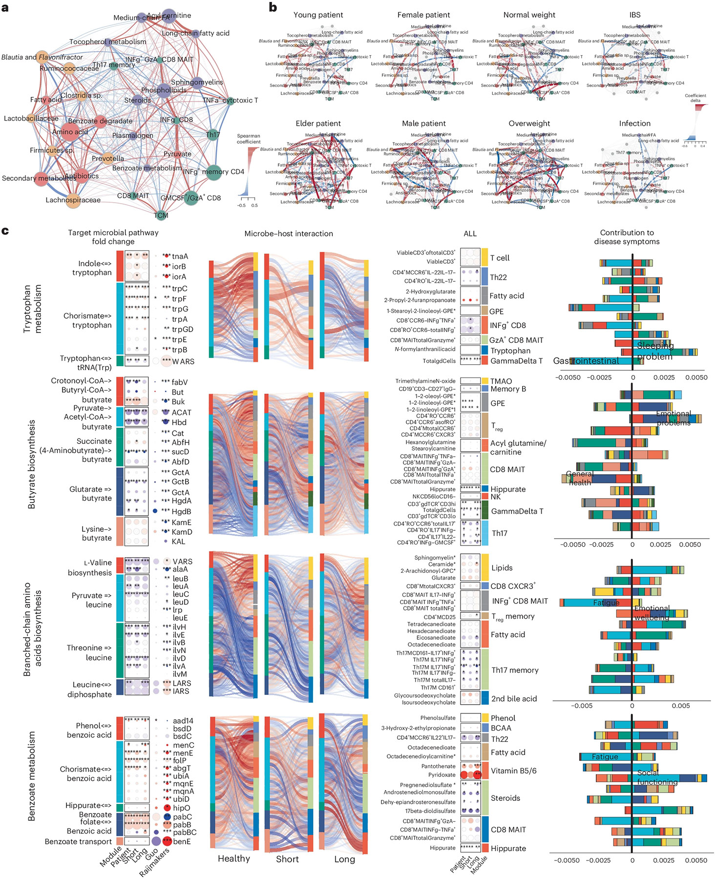
a,b, Microbiome-immune-metabolome network in healthy (a) and patient (b) subgroups. A baseline network was established with 200+ healthy control samples (a), bifurcating into two segments: the gut microbiome (species in yellow, genetic modules in orange) and blood elements (immune modules in green, metabolome modules in purple). Nodes: modules; size: number of members; colors: omics type; edges: interactions between modules, with Spearman coefficient (adjusted) represented by thickness, transparency and color—positive (red) and negative (blue). Here, key microbial pathways (pyruvate, amino acid and benzoate) interact with immune and metabolome modules in healthy individuals. Specifically, these correlations were disrupted in patient subgroups (b), as a function of gender, age (young <26 years versus older >50 years), BMI (normal <26 versus overweight >26) and health status (individuals with IBS or infections). Correlations significantly shifted from healthy counterparts (Extended Data Fig. 6c) are highlighted with colored nodes and edges indicating increased (red) or decreased (blue) interactions. c, Targeted microbial pathways and host interactions. Four microbial metabolic mechanisms were analyzed to compare control, short- and long-term patients with ME/CFS, and external cohorts for validation (Guo¹⁷ and Raijmakers¹⁸) along with their associated host immune/metabolome modules. 1. Microbial pathway fold change: key genes were grouped and annotated in subpathways. Circle size: fold change over control; color: increase (red) or decrease (blue), P values (patient versus control, P value by two-sided Wilcoxon, FDR adjusted; detailed statistics in Supplementary Table 8) marked. 2. Microbiome–host interactions: Sankey diagrams visualize interactions between microbial pathways and host immune cells/metabolites. Line thickness and transparency: Spearman coefficient (adjusted); color: red (positive), blue (negative). 3. Immune and metabolites fold change: pathway-correlated immune cells and metabolites are grouped by category. 4. Contribution to disease symptoms: stacked bar plots show accumulated SHAP values (contributions to symptom severity) for each disease symptom (1–12, as in Supplementary Table 1). Colors: microbial subpathways and immune/metabolome categories match module color in fold change maps. $x$ axis: accumulated SHAP values (contributions) from negative to positive, with the most contributed symptoms highlighted. P values: *P < 0.05, **P < 0.01, ***P < 0.001.

Healthy control-derived interactions, such as the microbial pyruvate module associating with multiple immune modules, and connections between commensal gut microbes (Prevotella, Clostridia sp., Ruminococcaceae) with Th17 memory cells, plasma steroids, phospholipids and tocopherol (vitamin E) (Fig. 4a), were disrupted in patients with ME/CFS. Increased correlations between gut microbiome and mucosal/inflammatory immune modules, including CD8⁺ MAIT and IFN-γ⁺ CD4 memory cells, suggested an increased association with microbiome and inflammatory elements in ME/CFS (Extended Data Fig. 6d). Notably, these interactions could differ by age, gender and weight (Fig. 4b).

Further examining several microbial modules whose networks were dysbiotic in patients, we mapped the correlations of their metabolic subpathways to plasma metabolites and immune cells and detailed the collective associations with host phenotypes (Fig. 4c and Supplementary Table 8). We further validated these findings with two independent cohorts (Guo et al.¹⁷ and Raijmakers et al.¹⁸). For example, increased tryptophan metabolism, associated with gastrointestinal issues, lost its negative association with Th22 cells, and gained correlations with γδ T cells and the secretion of IFN-γ and GzA from CD8 and CD8⁺ MAIT cells. Several networks associated with emotional dysregulation and fatigue differed significantly in patients versus controls: decreased butyrate production and BCAA biosynthesis, which had opposite correlations with Th17 and regulatory T cells (T_reg cells); plasma lipids had more correlations with γδ T and CD8⁺ MAIT cells in patients; and microbial benzoate, which is synthesized by Clostridia sp.⁴¹ and then converted to hippurate in the liver⁴², was positively correlated with plasma hippurate in long-term patients with ME/CFS. These disrupted pathways also had modified associations with a variety of plasma metabolites including steroids, phenols, BCAAs, fatty acids and vitamins B5 and B6. Notably, short-term patients with ME/CFS presented a transitional profile, resembling an intermediate between controls and long-term ME/CFS.

Based on BioMapAI’s predictions and subsequent network analyses, we propose that some of the disease-specific changes in ME/CFS arise from disrupted associations between the gut microbiome, immune system, and metabolome (Fig. 5). Reduced relative abundances of key microbes—such as Faecalibacterium prausnitzii—and corresponding disturbances in microbial metabolic pathways (for example, butyrate, tryptophan and BCAA production) correlated with pain and gastrointestinal abnormalities in ME/CFS. In healthy controls, these microbial metabolites are associated with activity of mucosal immune cells, including Th17, Th22 and T_reg cells. In ME/CFS, however, these regulatory networks break down, with heightened proinflammatory responses mediated by γδ T cells and CD8 MAIT cells producing IFN-γ and GzA, which in turn were associated with subjective health perception and social functioning.

Fig. 5 ∣. Overview of dysbiotic host–microbiome interactions in ME/CFS.

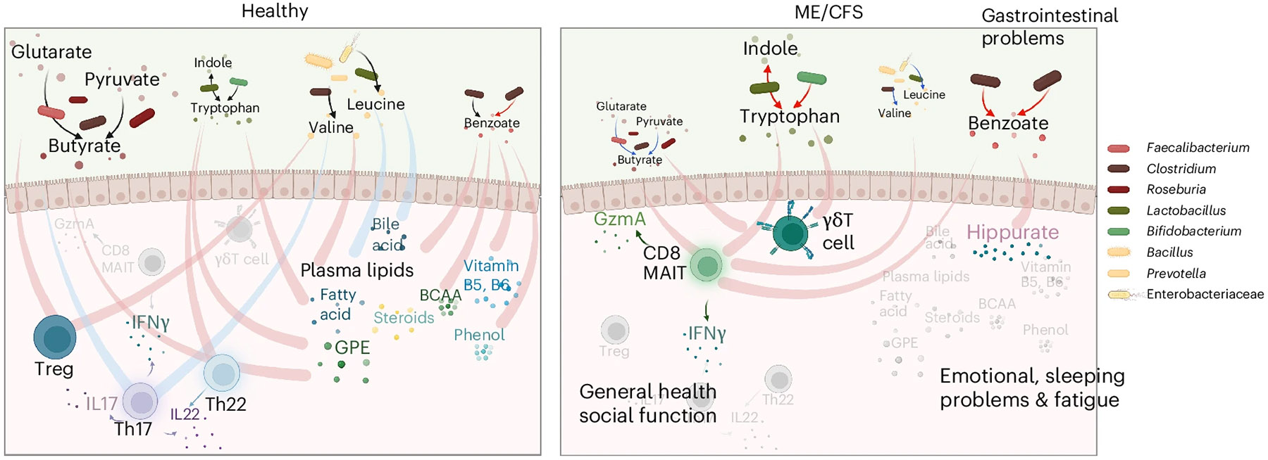
This conceptual diagram visualizes the host–microbiome interactions in healthy conditions (left) and its disruption and transition into the disease state in ME/CFS (right). The base icons of the figure remain consistent, whereas gradients and changes in color and size visually represent the progression of the disease. Process of production and processing is represented by lines with arrows, where the color indicates an increase (red) or decrease (blue) in the pathway in disease; lines without arrows indicate correlations, with red representing positive and blue representing negative correlations. In healthy conditions, microbial metabolites support immune regulation, maintaining mucosal integrity and healthy inflammatory responses by positively regulating T_reg and Th22 cell activity, and controlling Th17 activities, including the secretion of IL-17 (purple cells), IL-22 (blue) and IFN-γ. These microbial metabolites also maintain many positive interactions with plasma metabolites like lipids, bile acids, vitamins and phenols. In ME/CFS, there is a significant decrease in beneficial microbes and a disruption in metabolic pathways, marked by a decrease in the butyrate (brown-red dots) and BCAA (yellow) pathways and an increase in tryptophan (green) and benzoate (red) pathways. These changes are linked to gastrointestinal issues. In ME/CFS, the regulatory capacity of the immune system diminishes, leading to the loss of health-associated interactions with Th17, Th22 and T_reg cells, and an increase in inflammatory immune activity. Pathogenic immune cells, including CD8 MAIT and γδT cells, show increased activity, along with the secretion of inflammatory cytokines such as IFN-γ and GzmA, contributing to worsened general health and social functioning. Healthy interactions between gut microbial metabolites and plasma metabolites weaken or even reverse in the disease state. A notable strong connection increased in ME/CFS is benzoate transformation to hippurate, associated with emotional disturbances, sleep issues, and fatigue. Created in BioRender. Xiong, R. (2025) https://BioRender.com/cje1xlx.

Additional health-associated interactions between microbial benzoate metabolism and various plasma metabolites (for example, lipids, glycerophosphoethanolamine, fatty acids, and bile acids) we hypothesized are also diminished or reversed in ME/CFS. This breakdown in host–microbiome metabolic networks correlates with more severe fatigue, emotional disturbances, and sleep problems, aligning with emerging evidence that microbially derived metabolites may affect the gut–brain axis^43-45.

Discussion

Democratization of AI technologies and large-scale multi-omics has the promise of revolutionizing precision medicine⁴⁶. This study generated among the most extensive paired multi-omics dataset for ME/CFS to date^17-20,47, bringing unique technical and biological insights. Technically, BioMapAI marks a unique supervised DL model trained to accommodate these complex, multisystem ME/CFS symptoms. The rationale behind BioMapAI is that understanding long-term, post-infection syndromes like ME/CFS is not necessarily solved by pinpointing an exact diagnosis or tracing disease origins⁴⁸, but rather by addressing the chronic, multifaceted symptoms that substantially impacts patients’ quality of life⁴⁹. Biologically, our study introduces a highly nuanced approach to link physiological changes in gut microbiome, plasma metabolome, and immune status, with host symptoms, moving beyond the initial causes of the disease^50,51. Importantly, we validated key biomarkers in external cohorts^17-20, despite significant demographic and methodological differences between the studies.

This study represents a substantial technical and biological advance over our previous work and other investigations of ME/CFS to date. First, we developed BioMapAI, a supervised DNN architecture that accommodates the full complexity of our multi-omics data-sets—encompassing gut microbiome, plasma metabolome, immune profiling, blood labs, and extensive clinical surveys—beyond what traditional ML models can handle. By jointly modeling these diverse data types, BioMapAI explains the phenotypic heterogeneity of ME/CFS more effectively than single-outcome methods and simultaneously identifies symptom-specific biomarkers. Furthermore, our dataset’s unprecedented size, in both participant numbers and the depth of data types, allowed us to build an AI model validated on both held-out data and external cohorts. As a sanity check, we confirmed key biomarkers—such as altered Faecalibacterium prausnitzii and butyrate producers (reported by Guo et al.) as well as sphingolipid pathway changes (described by Raijmakers et al., Germain et al. and Che et al.)—using independent datasets, which other studies have not performed. Nonetheless, we acknowledge a caveat of our model is that distinguishing ME/CFS from healthy controls may be less challenging than differentiating ME/CFS from other conditions with overlapping symptoms, such as fibromyalgia. Future studies with comparative disease datasets are needed to assess this.

Second, we added a unique, detailed blood immune-profiling dataset, which provided the most biologically explanatory features for both disease classification and symptom severity. Leveraging these data, we were able to construct unique microbiome–metabolome–immune networks in both health and ME/CFS—an advance over earlier investigations that generally focused on only one omics layer (for example, stool microbiome in Guo et al.; plasma metabolomics in Germain et al. and Che et al.). Although Raijmakers et al. examined 92 inflammatory circulating markers, plasma metabolites and gut microbiome in a smaller study ($n=50\text{ME}∕\text{CFS}$, $n=72$ healthy control for metagenomics, and $n=22$ for metabolomics), their analyses were relatively limited in that they used ML models to differentiate ME/CFS from controls and only examined fatigue as a clinical variate, not adjusting for other clinical variables that could affect omics associations such as age, gender, or BMI. Moreover, their approach only assessed pairwise associations among data types. In contrast, our multi-omics strategy explicitly accounts for demographic and clinical covariates like age, gender and BMI, revealing that these factors can markedly reshape immune–microbiome–metabolome interaction networks, just as comorbid conditions such as obesity or advanced age can further individualize disease phenotypes.

Taken together, our dataset uncovers an array of correlations that although not causal, can further our understanding of ME/CFS in several ways. First, our analyses underscore the importance of considering clinical symptom heterogeneity and cohort-level covariates because interactions among the microbiome, metabolome, and immune system vary substantially depending on these factors. Although it has long been assumed that confounders play a major role, previous studies have seldom controlled for them in a comprehensive manner, potentially explaining some of the inconsistencies reported in single-omics analyses. Second, although our findings are correlative rather than causal, they generate numerous hypotheses about both specific and more extensive pathways that may be disrupted in ME/CFS.

For example, our previous analysis, and work by Guo et al., suggest that diminished butyrate-producing microbes in ME/CFS lower the availability of short-chain fatty acids (SCFAs) in the stool (Guo) and plasma (Xiong). Here, we refine that hypothesis by pinpointing potential immunological or metabolic mediators of this change. In healthy controls, multiple butyrate biosynthesis routes are inversely associated with Th17 cells, whereas the glutarate→butyrate pathway aligns with T_reg cells. These patterns become largely reversed in long-term disease, with succinate→butyrate showing unique negative correlations to T_reg cells and positive links with CD8⁺ MAIT cells. ME/CFS also substantially alters metabolite associations with Th17 cells. On the metabolomic side, there is currently no direct biochemical link reported between glutarate→butyrate and glycerophosphoethanolamine—though in healthy controls, they exhibited a strong positive correlation that was altered in ME/CFS. One can then hypothesize an indirect link with phospholipid metabolism and its effect on neurotransmission.

In addition to refining established hypotheses, our results propose unique links among tryptophan metabolism, BCAAs and benzoate metabolism in shaping immune function and symptomatology in ME/CFS. Although no direct biochemical connection between tryptophan metabolism and 2-hydroxyglutarate is currently known, both pathways likely influence immune regulation and metabolic reprogramming, indicating a more complex regulatory landscape. In healthy controls, tryptophan metabolism is closely tied to various T cell subsets, including Th22 cells, whereas these relationships are disrupted in ME/CFS. Furthermore, we observed significant alterations in benzoate metabolism modules and their associations with plasma steroids, hippurate, and fatty acids. These pathways, linked to both steroid biosynthesis and neurotransmitter production (for example, serotonin or cortisol), highlight a potential gut–brain axis component in ME/CFS pathophysiology.

Although some of these findings may seem granular or only indirectly testable (such as potential sex differences in the interaction network), our detailed, multi-omics perspective is valuable for unraveling the disease’s heterogeneity. As experimental models attempt to validate these hypotheses, one must keep in mind that many interactions may be context or model specific rather than universally turned on or off in disease states. This context dependency underscores the need for nuanced, carefully controlled mechanistic studies that incorporate patient heterogeneity and environmental factors when investigating ME/CFS.

Additional limitations of our study include that that our study population comprised more females and older individuals, most of whom were white (though this is consistent with the epidemiology of ME/CFS¹⁰), and was from a single geographic location (Bateman Horne Center), which may limit our findings to certain populations. In addition, previous RNA sequencing studies have suggested mitochondrial dysfunction and altered energy metabolism in ME/CFS^52,53; thus, incorporating host PBMC RNA or ATAC sequencing in future research could provide deeper insights into regulatory changes. The typical decades-long disease progression of ME/CFS makes it challenging for our 4-year longitudinal design to capture stable temporal signals (although separating our short-term (<4 years) and longterm (>10 years) provided valuable insights); ideally, tracking the same patients over a longer period would likely yield more accurate trends⁵⁴. Long disease history also increases the likelihood of exposure to various diets and medications⁵⁵, which could influence biomarker identification, particularly in metabolomics. Finally, model-wise, Bio-MapAI was trained on <500 samples with tenfold cross-validation, which is relatively small given the complexity of the outcome matrix; expanding the training dataset and incorporating more independent validation sets could potentially enhance its performance and prediction accuracy⁵⁶. Currently, the model treated all 12 studied symptoms with equal importance due to the unclear symptom prioritization in ME/CFS⁵⁷. We computed modules to assign different weights to symptoms to enhance diagnostic accuracy. Although this approach was not particularly effective for ME/CFS, it may be more promising for diseases with more clearly defined symptom hierarchies⁵⁸. In such cases, adjusting the weights of symptoms in the model’s final layer could improve performance and help pinpoint which symptoms more strongly contributing.

Although our findings are still preliminary for direct therapeutic application, the nuanced insights and deconstructed approach described here offer numerous hypotheses for dysbiotic microbiome–metabolome–immune connections in ME/CFS. We hope that the unprecedented systems-level resolution of our dataset, algorithm, and analyses will contribute to filling out heretofore unknown links between these factors thus explaining some of the disease heterogeneity in this important disease.

Methods

Study design

This was 4-year prospective study. All participants had a physical examination at the baseline visit that included evaluation of vital signs, BMI, orthostatic vital signs, skin, lymphatic system, HEENT, pulmonary, cardiac, abdomen, musculoskeletal, nervous system and fibromyalgia tender points. We enrolled a total of 153 patients with ME/CFS (of which 75 had been diagnosed with ME/CFS < 4 years before recruitment and 78 had been diagnosed with ME/CFS > 10 years before recruitment) and 96 healthy controls. Among them, 110 patients and 58 healthy controls were followed 1 year after the recruitment as timepoint 2; 81 patients and 13 healthy controls were followed 2 years after the recruitment as timepoint 3; and 4 patients were followed 4 years after the recruitment as timepoint 4. Subject characteristics are shown in Supplementary Table 1 and Extended Data Fig. 1a.

Medical history and concomitant medications were documented. Blood samples were obtained before orthostatic and cognitive testing. The 10-min NASA Lean Test and cognitive testing were conducted after the physical examination and blood draw⁵⁹. Cognitive efficiency was tested with the DANA Brain Vital, measuring three reaction time and information processing measurements⁶⁰. The orthostatic challenge was assessed with the 10-min NASA Lean Test. Participants rested supine for 10 min, and baseline blood pressure and heart rate were measured twice during the last 2 min of rest⁶¹.

Participants were provided with an at-home stool collection kit at the end of each in-person visit. The following questionnaires were completed at baseline: DePaul Symptom Questionnaire (DSQ), Post-Exertional Fatigue Questionnaire, RAND-36, Fibromyalgia Impact Questionnaire-R, ACR 2010 Fibromyalgia Criteria Symptom Questionnaire, Pittsburgh Sleep Quality Index, Stanford Brief Activity Survey, Orthostatic Intolerance Daily Activity Scale, Orthostatic Intolerance Symptom Assessment, Brief Wellness Survey, Hours of Upright Activity (HUA) and medical history and family history. All but medical history and family history were administered again when participants came for their annual visit.

Approval was received before enrolling any subjects in the study (The Jackson Laboratory Institutional Review Board, 17-JGM-13). All participants were educated about the study before enrollment and signed all appropriate informed consent documents. Research staff followed Good Clinical Practices (GCP) guidelines to ensure subject safety and privacy.

ME/CFS cohort

Beginning in January 2018, we enrolled patients with ME/CFS who had been sick for <4 years or sick for >10 years. No patients with ME/CFS with duration ≥4 years and ≤10 years were enrolled to have clear distinctions between short and long duration of illness with ME/CFS. All participants were 18 to 65 years old at the time of enrollment. ME/CFS diagnosis according to the Institute of Medicine clinical diagnostic criteria and disease duration of <4 years were confirmed during clinical differential diagnosis and thorough medical work up⁶². Additional inclusion criteria required 1) a substantial reduction or impairment in the ability to engage in pre-illness levels of occupational, educational, social or personal activities that persists for more than 6 months and less than 4 years and is accompanied by fatigue, which is often profound, is of new or definite onset (not lifelong), is not the result of ongoing excessive exertion, and is not substantially alleviated by rest, and 2) post-exertional malaise. Exclusionary criteria for the <4 years ME/CFS cohort were 1) morbid obesity BMI > 40; 2) other active and untreated disease processes that explain most of the major symptoms of fatigue, sleep disturbance, pain, and cognitive dysfunction; 3) untreated primary sleep disorders; 4) rheumatological disorders; 5) immune disorders; 6) neurological disorders; 7) infectious diseases; 8) psychiatric disorders that alter perception of reality or ability to communicate clearly or impair physical health and function; 9) laboratory testing or imaging are available that support an alternate exclusionary diagnosis; and 10) treatment with short-term (less than 2 weeks) antiviral or antibiotic medication within the past 30 days.

For the >10 years ME/CFS cohort, disease duration of >10 years and clinical criteria were confirmed to meet the Institute of Medicine criteria for ME/CFS during clinical evaluation and medical history review⁶². Other than disease duration, inclusion and exclusion criteria were the same as for <4 years ME/CFS cohort.

Healthy control cohort

Healthy control participants were also between 18 to 65 years and in general good health. Enrollment began in 2018 and subjects were selected to match the <4 years ME/CFS cohort by age (within 5 years), race, and sex (~2:1 female to male ratio). Exclusion criteria for healthy controls included, 1) a diagnosis or history of ME/CFS, 2) morbid obesity BMI > 40, 3) treatment with short-term (less than 2 weeks) antiviral or antibiotic medication within the past 30 days, or 4) treatment long-term (longer than 2 weeks) antiviral medication or immunomodulatory medications within the past 6 months.

Clinical metadata and scores

Clinical symptoms and baseline health status were assessed on the day of physical examination and biological sample collection for both case and control subjects. For each participant, we collected demographic information (including age, gender, diet, race, BMI, family, work, and education), medical histories, clinical tests and questionnaires. From questionnaires and test as described above, we summarized 12 clinical scores to cover major symptoms of ME/CFS: Scores 1–8 were derived from the RAND-36, following standardized rules⁶³ and summarized into eight categories: Physical Functioning (also referred to as Daily Activity in the main contents), Role Limitations due to Physical Health (Physical Limitations), Role Limitations due to Emotional Problems (Emotional Problems), Energy/Fatigue, Emotional Well-being (Mental Health), Social Functioning (Social Activity), Pain, and General Health (Health Perception). Cognitive Efficiency was summarized from the DANA Brain Vital test, Orthostatic Intolerance from the NASA Lean Test, Sleeping Problem Score from the Pittsburgh Sleep Quality Index questionnaire and Gastrointestinal Problems Score from the Gastrointestinal Symptom Rating Scale questionnaire. Each score was transformed into a 0–1 scale to facilitate combination and comparison, where a score of 1 indicates maximum disability or severity and a score of 0 indicates no disability or disturbance.

Plasma sample collection and preparation

Healthy and patient blood samples were obtained from Bateman Horne Center and approved by JAX IRB. One 4 ml lavender top tube (K2EDTA) was collected, and tube slowly inverted 8–10 times immediately after collection. Blood was centrifuged within 30 min of collection at 1,000g with low brake for 10 min. Then, 250 μl plasma was transferred into three 1 ml cryovial tubes, and tubes were frozen upright at −80 °C. Frozen plasma samples were batch shipped overnight on dry ice to The Jackson Laboratory and stored at −80 °C. Heparinized blood samples were shipped overnight at room temperature. PBMCs were isolated using Ficoll-paque plus (GE Healthcare) and cryopreserved in liquid nitrogen.

Plasma untargeted metabolome by UPLC-MS/MS

Plasma samples were sent to Metabolon platform and processed by Ultrahigh performance liquid chromatography-tandem mass spectroscopy (UPLC-MS/MS) following the CFS cohort pipeline. In brief, samples were prepared using the automated MicroLab STAR system from Hamilton Company. The extract was divided into five fractions: two for analysis by two separate reverse phases (RP)/UPLC-MS/MS methods with positive ion mode electrospray ionization (ESI), one for analysis by RP/UPLC-MS/MS with negative ion mode ESI, one for analysis by HILIC/UPLC-MS/MS with negative ion mode ESI and one sample was reserved for backup. Quality assurance/quality control were analyzed with several types of controls were analyzed including a pooled matrix sample generated by taking a small volume of each experimental sample (or alternatively, use of a pool of well-characterized human plasma), extracted water samples, and a cocktail of quality control standards that were carefully chosen not to interfere with the measurement of endogenous compounds were spiked into every analyzed sample, allowed instrument performance monitoring, and aided chromatographic alignment. Compounds were identified by comparison to Metabolon library entries of purified standards or recurrent unknown entities. The output raw data included the annotations and the value of peaks quantified using area under-the curve for metabolites.

Immune profiling flow cytometry analysis

Frozen PBMC aliquots were thawed, counted, and divided into two parts: one part for day 0 surface staining, and the other cultured in complete RPMI 1640 medium (RPMI plus 10% FBS and 1% penicillin/streptomycin (Corning Cellgro)) supplemented with IL-2 + IL-15 (20 ng ml⁻¹) for T_reg subsets. Day 1 surface and transcription factor staining followed culture with IL-7 (20 ng ml⁻¹) for day 1 and day 6 intracellular cytokine staining, and a combination of cytokines (20 ng ml⁻¹ IL-12, 20 ng ml⁻¹ IL-15 and 40 ng ml⁻¹ IL-18) for day 1 intracellular cytokine staining (IL-12 from R&D, IL-7 and IL-15 from BioLegend).

Surface staining was performed in PBS + 2% FBS for 30 min at 4 °C. When staining chemokine receptors, incubation was done at room temperature. Antibodies used in surface staining (all obtained from BioLegend) were used at a working stock concentration of approximately 0.5 mg ml⁻¹: 2B4, CD1c, CD14, CD16, CD19, CD25, CD27, CD31, CD3, CD303, CD38, CD4, CD45RO, CD56, CD8, CD95, CD161, CCR4, CCR6, CCR7, CX3CR1, CXCR3, CXCR5, γδ TCR (biotin-conjugated), HLA-DR, IgG, IgM, LAG3, PD1, TIM3, Va7.2 and Va24Ja18.

For intracellular cytokine staining, cells were stimulated with PMA (40 ng ml⁻¹ for overnight cultured cells and 20 ng ml⁻¹ for 6-day cultured cells) and Ionomycin (500 ng ml⁻¹) (both from Sigma-Aldrich) in the presence of GolgiStop (BD Biosciences) for 4 h at 37 °C. For cytokine secretion after stimulation with IL-12 + IL-15 + IL-18, GolgiStop was added to the culture on day 1 for 4 h. Following surface staining with markers (CD3, CD4, CD8, CD161, PD1, 2B4, Vα7.2, CD45RO, CCR6, CD27), cells were washed with PBS and stained with fixable viability dye (eBioscience), fixed, and permeabilized using buffers from eBioscience according to manufacturer instructions. Intracellular antibodies from BioLegend were used at working concentrations of approximately 0.2 mg ml⁻¹: FOXP3, Helios, IL-4, IFN-γ, TNF-α, IL-17A, IL-22, Granzyme A, GM-CSF and Perforin.

Flow cytometry was performed using Cytek Aurora (Cytek Biosciences) and analyzed with FlowJo (Tree Star). The gating strategy used involved setting preliminary FSC/SSC gates of the starting cell populations, followed by defining boundaries between ‘positive’ and ‘negative’ staining cell populations. Detailed gating strategies are provided in the Supplementary Fig. 2.

Fecal sample collection and DNA extraction

Stool was self-collected at home by volunteers using a BioCollector fecal collection kit (The BioCollective) according to manufacturer instructions for preservation for sequencing before sending the sample in a provided Styrofoam container with a cold pack. Upon receipt, stool and OMNIgene samples were immediately aliquoted and frozen at −80 °C for storage. Before aliquoting, OMNIgene stool samples were homogenized by vortexing (using the metal bead inside the OMNIgene tube), and then divided into two microfuge tubes, one with 100 μl aliquot and one with 1 ml. DNA was extracted using the Qiagen QIAamp 96 DNA QIAcube HT Kit with the following modifications: enzymatic digestion with 50 μg lysozyme (Sigma) and 5 U each of lysostaphin and mutanolysin (Sigma) for 30 min at 37 °C followed by bead-beating with 50 μg 0.1 mm of zirconium beads for 6 min on the Tissuelyzer II (Qiagen) before loading onto the Qiacube HT. DNA concentration was measured using the Qubit high-sensitivity dsDNA kit (Invitrogen).

Metagenomic shotgun sequencing

Approximately 50 μl thawed OMNIgene preserved stool sample was added to a microfuge tube containing 350 μl Tissue and Cell lysis buffer and 100 μg 0.1 mm zirconia beads. Metagenomic DNA was extracted using the QiaAmp 96 DNA QiaCube HT kit (Qiagen, 5331) with the following modifications: each sample was digested with 5 μL of Lysozyme (10 mg ml⁻¹, Sigma-Aldrich, L6876), 1 μl lysostaphin (5,000 U ml⁻¹, Sigma-Aldrich, L9043) and 1 μl Mutanolysin (5,000 U ml⁻¹, Sigma-Aldrich, M9901) were added to each sample to digest at 37 °C for 30 min before the bead-beating in the in the TissueLyser II (Qiagen) for 2 ×3 min at 30 Hz. Each sample was centrifuged for 1 min at 15,000g before loading 200 μl into an S-block (Qiagen, 19585) Negative (environmental) controls and positive (in-house mock community of 26 unique species) controls were extracted and sequenced with each extraction and library preparation batch to ensure sample integrity. Pooled libraries were sequenced over 13 sequencing runs using both HiSeq ($n=87$) and NovaSeq ($n=392$) platforms. To address potential biases arising from varying read depths, all samples were down-sampled, using seqtk (v1.3-r106), to 5 million reads. This threshold corresponds to the 95th percentile of the read count distribution across the dataset.

Sequencing adapters and low-quality bases were removed from the metagenomic reads using scythe (v0.994) and sickle (v1.33), respectively, with default parameters. Host reads were removed by mapping all sequencing reads to the hg19 human reference genome using Bowtie2 (v2.3.1), under ‘very-sensitive’ mode. Unmapped reads (that is, microbial reads) were used to estimate the relative abundance profiles of the microbial species in the samples using MetaPhlAn4.

Taxonomic profiling (species abundance) and KEGG gene profiling

Taxonomic compositions were profiled using Metaphlan4.0 (ref. 64) and the species whose average relative abundance > 1e-4 were kept for further analysis, giving 384 species. The gene profiling was computed with USEARCH⁶⁵ (v8.0.15) (with parameters: evalue 1e-9, accel 0.5, top_hits_only) to KEGG Orthology (KO) database v54, giving a total of 9,452 annotated KEGG genes. The reads count profile was normalized by DeSeq2 (ref. 66) in R. Genes with a prevalence of over 20%, meaning expressed in more than 20% of samples, were selected for downstream analysis.

Confounder analysis

Confounder analysis was done by R package MaAsLin2. We considered demographic features (including age, gender, BMI, ethnicity and race), diet records, medications (antivirals, antifungals, antibiotics and probiotics) and self-reported irritable bowel syndrome (IBS) scores as potential confounders. The analysis followed the model formula:

$$\begin{gathered} expr\sim \text{age}+\text{gender}+\text{bmi}+\text{ethnic}+\text{race}+\text{IBS}+\text{diet}\_\text{meat} \\ +\text{diet}\_\text{sugar}+\text{diet}\_\text{veg}+\text{diet}\_\text{grains}+\text{diet}\_\text{fruit}+\text{antifungals} \\ +\text{antibiotics}+\text{probiotics}+\text{antivirals}+(1\mid \text{sample}\_\text{id}\_\text{tp1}) \end{gathered}$$

where $expr$ refers to the omics matrix. For each feature in the omics data, we ran this generalized linear model to identify multivariable associations between each omics feature and each metadata feature. Identified confounders were handled differently based on the type of data. For species and KEGG genes, any feature with a significant statistical association with any metadata feature was removed from all subsequent analyses, resulting in the removal of 21 species and 946 microbial genes. For immune profiling and plasma metabolomics, to remove the effects of identified confounders, each feature was adjusted by retaining the residuals⁶⁴, that is, the part of the outcome not explained by the confounding factors, from a general linear model:

$$y^{\prime }=(y\sim \text{predicted confounders})\$\text{residual}$$

Additionally, for network and patient subset analysis (Methods), age, gender, BMI and IBS were not included as confounders, as we analyzed different age groups, gender groups, weight groups and IBS groups separately. However, other identified confounders were still considered in the residual models.

BioMapAI

The rationale behind BioMapAI is we believe that ME/CFS is characterized by significant heterogeneity and individual variability, making traditional approaches such as classifying patients versus controls and reporting single-disease biomarkers insufficient to us. This motivated us to develop a sophisticated model that directly integrates rich biological multi-omics data with clinical phenotypes. The primary learning goal of BioMapAI is to connect high-dimensional biology data, $X$ to mixed-type output matrix, $Y$. Unlike traditional ML or DL classifiers that typically predict a single outcome, $y$, BioMapAI is designed to learn multiple objects, $Y=[y_1,y_2,\dots ,y_n]$, simultaneously within a single model. This approach allows for the simultaneous prediction of diverse clinical outcomes (including binary, categorical and continuous variables) with omics profiles, thus addressing disease heterogeneity by tailoring each patient’s specific symptomology. The uniqueness of BioMapAI is it is a supervised DL model that integrates omics directly with clinical phenotypes in ME/CFS. This design enables simultaneous identification of symptom-specific and disease-general biomarkers, accounting for ME/CFS’s phenotypic heterogeneity.

BioMapAI structure.

BioMapAI is a fully connected DNN framework comprising an input layer $X$, a normalization layer, three sequential hidden layers, $Z^1$, $Z^2$, $Z^3$ and one output layer $Y$.

Input layer ($X$) takes high-dimensional omics data, such as gene expression, species abundance, metabolome matrix, or any customized matrix like immune profiling and blood labs. Normalization layer standardizes the input features to have zero mean and unit variance, defined as

$$X^{\prime }=\frac{X-\mu }{\sigma }$$

where $\mu$ is the mean and $\sigma$ is the standard deviation calculated from training dataset. We used TensorFlow’s standard BatchNormalization function. During training, mean and variance were computed from each mini-batch, and the model maintained a moving average of these values over time. During inference, instead of recalculating statistics from the test data, the model used the moving average of the training mean and variance for normalization to ensure consistent feature scaling between training and inference.

Feature learning module is the core of BioMapAI, responsible for extracting and learning important patterns from input data. Each fully connected layer (hidden layer 1–3) is designed to capture complex interactions between features. Hidden layer 1 ($Z^1$) and hidden layer 2 ($Z^2$) contain 64 and 32 nodes, respectively, both with ReLU activation and a 50% dropout rate, defined as:

$$Z^k=\text{ReLU}(W^k{Z}^{k-1}+b^k),k\in \{1,2\}$$

Hidden layer 3 ($Z^3$) has $n$ parallel sublayers for each object, $y_i$ in $Y$. Every sublayer, $Z_i^3$, contains eight nodes, represented as:

$$Z_i^3=\text{ReLU}(W_i^3{Z}^3+b_i^3),i\in \{1,2,\dots ,n\}$$

All hidden layers used ReLU activation functions, defined as:

$$\text{ReLU}(x)=\max (0,x)$$

Outcome prediction module is responsible for the final prediction of the objects. The output layer ($Y$) has $n$ nodes, each representing a different object:

$$y_i=\{\begin{array}{c}\sigma (W_i^4{Z}_i^3+b_i^4)\text{for binary object}\hfill \\ \mathsf{softmax}(W_i^4{Z}_i^3+b_i^4)\text{for categorical object}\hfill \\ W_i^4{Z}_i^3+b_i^4\text{for continuous object}\hfill \end{array}\phantom{\}}$$

The loss functions are dynamically assigned based on the type of each object:

$$ℒ=\{\begin{array}{cc}\frac{1}{N}{\sum }_{i=1}^N[y_i\log ({\widehat{y}}_i)+(1-y_i)\log (1-{\widehat{y}}_i)\hfill & \text{for binary object}\hfill \\ -\frac{1}{N}{\sum }_{i=1}^N{\sum }_{j=1}^C{y}_{ij}\log ({\widehat{y}}_{ij})\hfill & \text{for categorical object}\hfill \\ \frac{1}{N}{\sum }_{i=1}^N\{\begin{array}{c}0.5{(y_i-{\widehat{y}}_i)}^2,\text{if}\mid y_i-{\widehat{y}}_i\mid \le \delta \hfill \\ \delta [y_i-{\widehat{y}}_i\mid -0.5{\delta }^2,\text{otherwise}\hfill \end{array}\phantom{\}}\hfill & \text{for continuous object}\hfill \end{array}\phantom{\}}$$

During training, the weights are adjusted using the Adam optimizer. The learning rate was set to 0.01, and weights were initialized using the He normal initializer. L2 regularizations were applied to prevent overfitting.

The optional binary classification layer is not used for parameter training. An additional binary classification layer is attached to the output layer $Y$ to evaluate the model’s performance in binary classification tasks. This layer is not used for training BioMapAI but serves as an auxiliary component to assess the accuracy of predicting binary outcomes, for example, disease versus control. This ScoreLayer takes the predicted scores from the output layer and performs binary classification:

$$y_{\text{binary}}=\sigma (W_{\text{binary}}Y+b_{\text{binary}})$$

The initial weights of the 12 scores are derived from the original clinical data, and the weights are adjusted based on the accuracy of BioMapAI’s predictions:

$$w_{\text{new}}=w_{\text{old}}-\eta \nabla {ℒ}_{\text{MSE}}$$

where $\nabla {ℒ}_{\text{MSE}}$ refers to the MSE between the predicted $y^{\prime }$ and true $y$; then the weights are adjusted to optimize the accuracy of the binary classification.

Training and evaluation of BioMapAI for ME/CFS BioMapAI:: DeepMECFS.

BioMapAI is a framework designed to connect highdimensional, sparse biological omics matrix $X$ to multi-output $Y$. Although BioMapAI is not tailored to a specific disease, it is versatile and applicable to a broad range of biomedical topics. In this study, we trained and validated BioMapAI using our ME/CFS datasets. The trained models are available on GitHub, nicknamed DeepMECFS, for the benefit of the ME/CFS research community.

To ensure uniform learning for each output $y$, it is crucial to address sample imbalance before fitting the framework. We recommend using customized sample imbalance handling methods, such as the synthetic minority over-sampling technique (SMOTE), adaptive synthetic (ADASYN) or random undersampling (RUS)⁶⁷. In our ME/CFS dataset, there is a significant imbalance, with the patient data being twice the size of the control data. To effectively manage this class imbalance, we used RUS as a random sampling method for the majority class. Specifically, we randomly sampled the majority class 100 times. For each iteration $i$, a different random subset $S_i^{\text{majority}}$ was used. This subset $S_i^{\text{majority}}$ of the majority class was combined with the entire minority class $S^{\text{minority}}$. For each iteration $i$:

$$\begin{gathered} S_i^{\text{majority}}\subseteq S^{\text{majority}},S^{\text{minority}}=S^{\text{minority}} \\ {S}_i=S_i^{\text{majority}}\cup S^{\text{minority}} \end{gathered}$$

where the combined dataset $S_i$ was used for training at each iteration. This approach allows the model to generalize better and avoid biases towards the majority class, improving overall performance.

Model training, cross-validation and held-out validation.

DeepMECFS is the name of the trained BioMapAI model with ME/CFS datasets. We trained on five preprocessed omics datasets, reporting DeepMECFS-Species for species abundances (feature $n=118$, sample $n=441$), DeepMECFS-KEGG for KEGG gene abundances (feature $n=3,959$, sample $n=441$) from the microbiome, DeepMECFS-Metabolome for plasma metabolome (feature $n=730$, sample $n=376$), DeepMECFS-Immune for immune profiling (feature $n=311$, sample $n=451$) and DeepMECFS-Quest for blood quest lab measurements (feature $n=48$, sample $n=465$). Additionally, an integrated omics profile was created by merging the most predictive features from each omics model related to each clinical score (SHAP, Methods), forming a comprehensive matrix of 154 features, comprising 50 immune features, 32 species, 30 KEGG genes and 42 plasma metabolites. The trained omics model is named DeepMECFS-Omics.

To evaluate the performance of BioMapAI, we used a 10-fold cross-validation alongside a held-out validation approach. Specifically, 10% of the data was excluded from the cross-validation process to serve as an independent validation set. This allowed us to assess both the model’s performance during cross-validation and its prediction accuracy on unseen data. Training was conducted over 500 epochs with a batch size of 64 and a learning rate of 0.0005, optimized through grid search. The Adam optimizer was used to adjust the weights during training, chosen for its ability to handle sparse gradients on noisy data. The initial learning rate was set to 0.0005, with beta1 set to 0.9, beta2 set to 0.999, and epsilon set to 1e-7 to ensure numerical stability. Dropout layers with a 50% dropout rate were used after each hidden layer to prevent overfitting, and L2 regularization ($\lambda =0.008$) was applied to the kernel weights, defined as:

$$L_{\text{reg}}=\frac{\lambda }{2}\sum _{i=1}^N{w}_i^2$$

To evaluate the performance of the models, we used several metrics tailored to both regression and classification tasks. The MSE was used to evaluate the performance of the reconstruction of each object. For each $y_i$, MSE was calculated as:

$${\text{MSE}}_i=\frac{1}{N}\sum _{j=1}^N{\left(y_i^j-{\widehat{y}}_i^j\right)}^2,i=1,2,\dots ,n$$

where $y_i^j$ is the actual values, ${\widehat{y}}_i^j$ is the predicted values, and $N$ is the number of samples, $n$ is the number of objects. For binary classification tasks (ME/CFS versus control), we utilized multiple metrics including accuracy, precision, recall, F1 score, AUC and area under the precision-recall curve to enable a comprehensive evaluation of the model’s performance.

To benchmark the performance of BioMapAI, we compared its binary classification performance with four traditional machine learning models and one DNN model. The traditional machine learning models included logistic regression (C = 0.5, saga solver with Elastic Net regularization); generalized linear modeling with elastic net regularization (Glmnet) (grid search for best alpha/lambda, tuneLength = 10) - R glmnet, caret; Glmnet with interaction terms (Glmnet-int) - R glmnet, caret; SVM with an RBF kernel (C = 2, parameters were selected using grid search with GridSearchCV from scikit-learn) - sklearn.svm.SVC; and gradient-boosting decision trees (learning rate = 0.05, maximum depth = 5, estimators = 1000, parameters were selected using grid search with GridSearchCV from scikit-learn) - sklearn.ensemble. GradientBoostingClassifier. DNN model used the same hyperparameters as BioMapAI, except it did not include the parallel sublayer, $Z_3$; thus it only performed binary classification instead of multi-output predictions. The comparison between BioMapAI and DNN aims to assess the specific contribution of the spread-out layer, designed for discerning object-specific patterns, in binary prediction. For fair comparisons among models, all traditional ML models was trained and evaluated on the exact same training datasets, test datasets and held-out datasets as DeepMECFS. Evaluation metrics are detailed in Supplementary Table 3.

For hyperparameter tuning of BioMapAI, we conducted a systematic hyperparameter tuning procedure to optimize BioMapAI’s performance on 12 symptom-specific clinical outcomes and disease status (ME/CFS versus control) using the training dataset, leaving the held-out dataset remained completely separate. Our goal was to balance predictive accuracy, model complexity, and generalizability across high-dimensional omics datasets. The results of our tuning experiments are illustrated in Supplementary Fig. 1. We began with a base BioMapAI architecture consisting of two shared hidden layers (each with 128 nodes), no dropout, no L2 penalty and training for 1,000 epochs.

We first investigated how varying the number of shared hidden layers (1, 2, 3 or 4) affected both clinical score prediction (MSE) and disease classification (accuracy). As shown in Supplementary Fig. 1a, two shared hidden layers achieved the best predictive performance.

Next, we performed a grid search over learning rates {0.01,0.00 1,0.0005,0.0001,0.00005,0.00001} and batch sizes {32,64,128}. We trained each configuration for 1,000 epochs using the Adam optimizer. Supplementary Fig. 1b (heatmaps) displays the MSE for each of the 12 clinical scores at different combinations of learning rate and batch size. A learning rate of 0.0005 and batch size 64 emerged as the optimal balance, yielding stable training curves and minimal variance across folds. Although we initially trained for 1,000 epochs, we observed that validation metrics consistently stabilized by around 500 epochs. To prevent overfitting and reduce computational burden, we introduced early stopping at 500 epochs in subsequent experiments.

We then tuned the number of neurons in each of the two shared hidden layers. Configurations tested included {256,128,64,32,16,8} for the first and the second layer. As shown in Supplementary Fig. 1c, whereas the 128–64 setting performed similarly to other higher-width combinations, we observed that 64–32 minimized overfitting risk yet retained predictive accuracy. Thus, we selected 64 neurons in the first shared layer and 32 in the second.

To further mitigate overfitting in the hidden layers, we examined dropout rates {0.1,0.2,0.5,0.8}. Supplementary Fig. 1c demonstrates that 0.5 offered the best overall balance. We therefore used a 50% dropout after each shared layer. Lastly, we tested L2 penalty strengths $\lambda \in \{0.1,0.05,0.01,0.005,0.008,0.001,0.0001\}$. A moderate penalty of $\lambda =0.008$ was selected (Supplementary Fig. 1e).

Our final chosen hyperparameters include: Two shared hidden layers with sizes 64 and 32, each followed by a ReLU activation and 50% dropout; Batch size = 64, 500 epochs with early stopping; An Adam optimizer (initial learning rate = 0.0005, $\beta 1=0.9$, $\beta 2=0.999$, $\epsilon =1\times {10}^{-7}$), L2 penalty $\lambda =0.008$. We observed that the model’s overall performance (MSE on symptom scores, accuracy for ME/CFS classification) was not highly sensitive to small deviations in these hyperparameters. Even with the baseline configuration (128 nodes, no dropout, no penalty), the predictive performance was reasonable; however, this final tuned setup led to an improvement of approximately 5–10% and yielded more stable and generalizable outcomes across the five omics datasets.

Sensitivity analyses of BioMapAI.

For sensitivity analysis of BioMapAI, we first re-trained our final BioMapAI configuration ten times with different random initializations. Classification metrics and regression metrics (MSE) for the twelve clinical outcomes were collected. As shown in Supplementary Table 2, the standard deviations were minimal (<5%) across these ten runs, indicating that BioMapAI is robust to changes in random seed initialization. We also evaluated three similarly performing model architectures (chosen based on grid search results) that yield near-identical or slightly different loss values: model 1: 128 nodes in the first shared layer, 32 nodes in the second shared layer, $\lambda =0.008$; model 2: 32 nodes in the first shared layer, 32 nodes in the second shared layer, $\lambda =0.008$; model 3: 64 nodes in the first shared layer, 32 nodes in the second shared layer, $\lambda =0.005$. As shown in Supplementary Table 2, whereas minor fluctuations in classification performance were observed, the results were genernally consistent. This underscores BioMapAI’s stability: adjusting the number of neurons in the shared layers or slightly altering the L2 penalty does not substantially degrade classification or regression outcomes. Collectively, these analyses confirm that BioMapAI’s core design is not overly sensitive to small architectural or regularization variations. Even when trained with alternative hyperparameter settings, the model yields consistent performance on both classification (ME/CFS versus control) and symptom severity score learning.

External validation with independent dataset.

To validate BioMapAI’s abilities in binary classification, we used four external cohorts^17-20 comprising more than 100 samples. For these external cohorts, only binary classification is available. A detailed summary of data collection for these cohorts is provided in Supplementary Table 6. For each external cohort, we processed the raw data (if available) using our in-house pipeline. The features in the external datasets were aligned to match those used in BioMapAI by reindexing the datasets. The overlap between the features in the external dataset and BioMapAI’s feature set was calculated to determine feature coverage. Any missing features were imputed with zeros to maintain consistency across datasets. The input data were then standardized as BioMapAI. We loaded the pre-trained BioMapAI, gradient-boosting decision tree and DNN for comparison. Logistic regression and SVM were excluded because they did not perform well during the in-cohort training process. The performance of the models was evaluated using the same binary classification evaluation metrics. Evaluation metrics detailed in Supplementary Table 3.

BioMapAI decode module SHAP.

BioMapAI is designed to be explainable, ensuring that it not only reconstructs and makes predictions but also is interpretable, which is particularly crucial in the biological domain. To achieve this, we incorporated SHAP into our framework. SHAP offers a consistent measure of feature importance by quantifying the contribution of each input feature to the model’s output⁶⁸.

We applied SHAP to BioMapAI to interpret the results, following these three steps:

1. Model reconstruction.

BioMapAI’s architecture includes two shared hidden layers ($Z^1$, $Z^2$) and one parallel sublayer ($Z_i^3$) for each object $y_i$. To decode the feature contributions for each object $y_i$, we reconstructed sub-models from single comprehensive model:

$${\text{Model}}_i=Z^1+Z^2+Z_i^3,i=1,2,\dots ,n$$

where $n$ is the number of learned objects.

2. SHAP Kernel Explainer.

For each reconstructed model, ${\text{Model}}_i$, we used the SHAP Kernel Explainer to compute the feature contributions. The explainer was initialized with the model’s prediction function and the input data $X$:

$${\text{explainer}}_i=\text{shap.KernelExplainer}({\text{Model}}_i.\text{predict},X),i=1,2,\dots ,n$$

Then, SHAP values were computed to determine the contribution of each feature to $y_i$:

$${\varphi }_i={\text{explainer}}_i(X),i=1,2,\dots ,n$$

The kernel explainer is a model-agnostic approach that approximates SHAP by evaluating the model with and without the feature of interest and then assigning weights to these evaluations to ensure fairness. For each ${\text{Model}}_i$, with each feature $j$:

$$\begin{gathered} {\varphi }_i^j(f,x)=\sum _{S_i\subseteq N_i\backslash \{j\}}\frac{\mid S_i\mid !(m-\mid S_i\mid -1)!}{m!}({\text{Model}}_i(S_i\cup j)-{\text{Model}}_i(S_i)) \\ =\frac{1}{m}\sum _{S_i\subseteq N_i\backslash \{j\}}{\left(\begin{array}{c}\hfill m-1\hfill \\ \hfill m-\mid S_i\mid -1\hfill \end{array}\right)}^{-1}({\text{Model}}_i(S_i\cup j)-{\text{Model}}_i(S_i)),i=1,2,\dots ,n \end{gathered}$$

where $n$ is the number of learned objects, $m$ is the total number of features, ${\varphi }_i^j$ is the Shapley value for feature $j$ in ${\text{Model}}_i$, $N_i$ is the full set of features in ${\text{Model}}_i$, $S_i$ is the subset of features not including feature $j$, ${\text{Model}}_i(S_i)$ is the model prediction for the subset $S_i$. The SHAP value matrix, ${\varphi }_i$, were further reshaped to align with the input data dimensions.

3. Feature vategorization.

Analyzing the SHAP value matrices, [${\varphi }_1,{\varphi }_2,\dots ,{\varphi }_n$] , features can be roughly assigned to two categories: shared features (important to all outputs) or specific features (specifically important to individual outputs). We set the cutoff at 75%, where features consistently identified as top contributors in 75% of the models were classified as shared important features, termed disease-specific biomarkers. Features that were top contributors in only a few models were classified as specific important features, termed symptom-specific biomarkers.

By reconstructing individual models, ${\text{Model}}_i$, for each object, $y_i$, and applying SHAP explainer individually, we effectively decoded the contributions of input features to BioMapAI’s predictions. This method allowed us to categorize features into shared and specific categories—termed as disease-specific and symptom-specific biomarkers—providing unique interpretations of the omics feature contribution to clinical symptoms.

Interaction types of important features included:

Linear (monotonic) relationship. A feature $x$ and a symptom $y$ follow a roughly linear (or strictly monotonic) trend when the change in $y$ can be approximated by a single slope over $x$’s range. Formally, $y\approx \alpha +\beta x$, with $\beta \ne 0$, implying a consistently increasing ($\beta >0$) or decreasing ($\beta <0$) trend. Biologically, as the biomarker goes up, the symptom steadily increases (positive $\beta$) or decreases (negative $\beta$).

A biomarker $x$ relates to a symptom $y$ through a two-phase pattern or biphasic relationship, such as a U-shaped or inverted U-shaped curve. One way to represent this is by including a squared term: $y\approx \alpha +\beta 1x+\beta 2x^2$, with $\beta 2\ne 0$. Biologically, this often reveals that both very low and very high biomarker values are associated with greater symptom severity, whereas moderate values relate to reduced severity (or vice versa).

Dispersed relationship. If there is no single coherent shape (linear or otherwise) that describes the biomarker–symptom relationship across all individuals. Instead, contributions may appear sparse (affecting only a small subset of participants) or highly variable with no dominant pattern. Biologically, this is a typical relationship at KEGG profile in our case, where different individuals can exhibit different directions or magnitudes of effect, leading to scattered or ‘patchy’ patterns.

To the stability of SHAP values under repeated experiments and similar model configurations, we conducted re-ran the same data with the same architecture (different random seeds) as above. We then computed the standard deviation of the SHAP values for each feature. Over 90% of features exhibit less than 3% variation in their SHAP contributions across runs, indicating that the top features remain highly consistent despite random seed variation.

We also computed SHAP values for each of the three alternative model architectures (model 1, model 2, model 3) described above. Despite their slight architectural or regularization differences, the top 50 features identified by SHAP largely overlapped with those from the final BioMapAI. Although some lower-ranked features did differ across models, those changes accounted for less than 5% of the total SHAP variance, suggesting that the core set of important predictors remains stable. Consequently, the minor variations observed are unlikely to affect clinical interpretation or downstream analyses. In summary, both random initializations and small architectural changes do not substantially alter the SHAP-based feature importance patterns in Bio-MapAI. The top features remain consistent, reinforcing the reliability and interpretability of our multi-output DL framework.

Packages and tools.

BioMapAI was constructed by Tensor-flow(v2.12.0) and Keras(v2.12.0). ML models were from scikit-learn(v 1.1.2), Glmnet models were using R package glmnet⁶⁹ (v4.1-4) and caret⁷⁰ (v6.0.93).

Usage of BioMapAI.

We have included our GitHub README.md file and introduced a Jupyter notebook for user instruction. Because there are limited large-scale multi-omics datasets with sufficient matched clinical data for us to test BioMapAI’s prediction accuracy, we have not trained BioMapAI on other disease states. However, BioMapAI’s specialized DNN structured with two shared general layers and one outcome-focused parallel layer should be generalizable and scalable to other cohort studies that aim to utilize omics data for a range of outputs (for example, not just limited to clinical symptoms). For instance, researchers could employ our model to link whole-genome sequencing data with blood or protein measurements. Constructed to automatically adapt to any input matrix and any output matrix, BioMapAI defaults to parallelly align specific layers for each output.

WGCNA and network analysis

To identify co-expressed patterns of each omics, we used WGCNA using the WGCNA⁷¹ package in R. The analysis was performed on preprocessed omics data (Methods): species abundances (feature $n=373$, sample $n=479$) and KEGG gene abundances (feature $n=4,462$, sample $n=479$) from the microbiome, plasma metabolome (feature $n=395$, sample $n=414$), immune profiling (feature $n=311$, sample $n=489$). Network construction and module detection involved choosing soft-thresholding powers tailored to each dataset: 6 for species, 7 for KEGG, 5 for immune, and 6 for metabolomic. The adjacency matrices were transformed into topological overlap matrices to reduce noise and spurious associations. Hierarchical clustering was performed using the topological overlap matrices, and modules were identified using the dynamic tree cut method with a minimum module size of 30 genes. Module eigengenes were calculated, and modules with highly similar eigengenes (correlation >0.75) were merged. Moduletrait relationships were assessed by correlating module eigengenes with clinical traits, and gene significance and module membership were used to identify hub genes within significant modules.

Network analysis was conducted using igraph⁷² in R. Module eigengenes from the WGCNA analysis were extracted for each dataset. A combined network was constructed by calculating Spearman correlation coefficients (corrected, Methods) between the module eigengenes of different datasets, and an adjacency matrix was created based on a threshold of 0.3 (absolute value) to include only significant associations. Network nodes represented module eigengenes and edges represented significant correlations. Degree centrality and betweenness centrality were calculated to identify highly connected and influential nodes. Networks in patient subgroups were displayed as the correlation differences from their healthy counterparts to exclude the influence of covariates. For example, correlations in female patients were compared with female healthy, and correlations in older patients were compared with older healthy.

Statistical analysis

Dimensionality reduction was performed using PCoA, implemented via the sklearn.manifold.MDS function in Python, applied separately to each omics dataset. For integrated analysis across omics layers, PCoA was applied to the combined module eigengenes obtained from WGCNA.

Differential abundance or expression analysis of microbial species, genes, immune cell populations, and metabolites was conducted across patient subgroups (short-term vs. control, long-term vs. control, and all patients vs. control). Group comparisons were carried out using the two-sided Wilcoxon rank-sum test. Resulting p-values were corrected for multiple hypothesis testing using the Benjamini–Hochberg FDR method unless otherwise specified.

Spearman’s rank correlation coefficients were computed using the scipy.stats.spearmanr function in Python. All correlation tests were two-sided, and corresponding P values were adjusted for multiple comparisons using the Holm–Bonferroni method. To estimate uncertainty in correlation estimates, 95% confidence intervals were calculated via bootstrap resampling (1,000 iterations). For each bootstrap iteration, random sampling with replacement was performed, and the Spearman correlation was recomputed; confidence bounds were defined as the 2.5th and 97.5th percentiles of the resulting distribution.

Statistical significance was annotated as follows: **P ≤ 0.001, *P ≤ 0.01, P ≤ 0.05, and n.s. (not significant) for P > 0.05.

Longitudinal analysis

To capture statistically meaningful temporal signals, we employed various statistical and modeling methods, accounting for both linear and nonlinear trends and intraindividual correlations:

1. IQR and intraclass correlation coefficient (ICC). We initially assessed statistics at different time points by computing the IQR and ICC. Data were standardized to a mean of zero and a standard deviation of one to ensure comparability across features with different scales. The IQR quantified variability, whereas the ICC assessed the dependence of repeated measurements⁷³, indicating the similarity of measurements over time. Data showed no statistical dependence and no trend of stable variance across time points.

2. Generalized linear models (GLMs). Generalized linear models⁷⁴ were then used to analyze the effects of time points, considering age, gender and their interactions. Time points were included as predictors to reveal changes in dependent variables over time, with interaction terms exploring variations based on age and gender. Random effects accounted for intraindividual correlations. Although 12 features out of 5,000 showed weak trends over time (slopes < 0.2), they were not deemed sufficient to be potential longitudinal biomarkers, possibly due to individualized patterns.

3. Repeated measures correlation (rmcorr). To better consider individual effects, we employed rmcorr⁷⁵ to assess consistent patterns of association within individuals over time. This method captured stable within-individual associations across different time points. However, only 30 features out of 5,000 showed weak slopes (<0.3), and these were not considered sufficient to conclude the presence of longitudinal signals.

4. Smoothing spline ANOVA (SS-ANOVA). We then considered the longitudinal trends could be nonlinear and more complex. To model complex, nonlinear relationships between response variables and predictors over time, SS-ANOVA⁷⁶ was used. SS-ANOVA uncovered nonlinear trends and interactions in the omics data, but no strong temporal signals were identified.

In conclusion, analysis of the longitudinal data, accounting for both linear and nonlinear trends and intraindividual correlations, revealed the difficulty in extracting strong and statistically meaningful temporal signals. As ME/CFS is a disease that usually lasts for decades with nonlinear progression, the 4-year tracking period with annual measurements is likely insufficient for capturing consistent temporal signals, necessitating longer follow-up periods.

In short, we observed that each patient exhibited independent patterns at each time point in both omics data and clinical symptoms (Fig. 1b and Extended Data Fig. 1). Based on these findings, we included each time point as an independent data point in BioMapAI. We applied this approach to increase the effective sample size, allowing the model to better capture associations between omics data and clinical symptoms.

Extended Data

Extended Data Fig. 1 ∣. Data Pairedness Overview and Heterogeneity in Healthy and Patients.

a, Cohort Composition and Data Collection. Over four years, 515 time points were collected: baseline year from all 249 donors (Healthy N=96, ME/CFS N=153); second year from 168 individuals (Healthy N=58, ME/CFS N=110); third year from 94 individuals (Healthy N=13, ME/CFS N=81); fourth year from N=4 ME/CFS patients. Clinical metadata and blood measures were collected at all 515 points. Immune profiles from PBMCs were recorded at 489 points, microbiome data from stool samples at 479 points, and plasma metabolome data at 414 points. A total of 1,471 biosamples were collected. b-c, Heterogeneity of b, Healthy Controls and c, All Patients in Symptom Severity and omics Profiles. Supplemental information for Fig. 1b, which shows examples from 20 patients. Variability in symptom severity (top) and omics profiles (bottom) for all healthy controls and all patients with 3-4 time points. The top x-axis numbers represent 12 symptoms, arranged in the same order as Extended Data Fig. 1f, g (left to right, top to bottom). d, Distribution of 12 Clinical Symptoms in ME/CFS and Control. Density plots compare the distributions of 12 clinical scores between control (blue) and ME/CFS patients (orange) with the x-axis represents the values of symptom severity (scaled from 0%, no symptom, to 100%, most severe) and the y-axis represents the frequency (count) of data points. e, Principal Coordinates Analysis (PCoA) of each ‘Omics. PCoA based on Bray-Curtis distance. Control samples (blue) and ME/CFS patients (red) show distinct clustering. Here, except for the clinical scores, controls are indistinguishable from patients, highlighting the difficulty of building classification models. f-g, Symptom Progression Over Time in f, Healthy vs. g, ME/CFS Patients. Symptom progression for each individual (represented by different colors) is shown using line plots of symptom severity (y-axis) over time points (years 1–4). Compared to healthy controls, ME/CFS patients exhibit higher severity, greater heterogeneity, and inconsistent or nonlinear progression (indicated by substantial variation over time without a consistent pattern) in clinical symptoms. Related to: Figs. 1-2.

Extended Data Fig. 2 ∣. BioMapAI’s Performance at Clinical Score Reconstruction and Disease Classification.

a, Density map of True vs. Predicted Clinical Scores. Supplemental information for Fig. 2b, which shows three examples. Here, the full set of 12 clinical scores compares the true score, $y$ (Column 1), against BioMapAI’s predictions generated from different omics profiles – ${\widehat{y}}_{immune}$, ${\widehat{y}}_{species}$, ${\widehat{y}}_{KEGG}$, ${\widehat{y}}_{metabolome}$, ${\widehat{y}}_{quest}$, ${\widehat{y}}_{omics}$ (Columns 2–7). b, Scatter Plot of True vs. Predicted Clinical Scores. Scatter plots display the relationship between true clinical scores (x-axis) and predicted clinical scores (y-axis) for six different models: Omics, Immune, Species, KEGG, Metabolome, and Quest Labs. Each plot demonstrates the clinical score prediction accuracy for each model. c, ROC Curve for Disease Classification with Original Clinical Scores. The Receiver Operating Characteristic (ROC) curve evaluates the performance of disease classification using the original 12 clinical scores. The mean Area Under the Curve (AUC) is 0.99, indicating high prediction accuracy, which aligns with the clinical diagnosis of ME/CFS based on key symptoms. d, 3D t-SNE Visualization of Hidden Layers. 3D t-SNE plots show how BioMapAI progressively distinguishes disease from control across hidden layers for five trained ‘omics models: Immune, KEGG, Species, Metabolome, and Quest Labs. Each plot uses the first three principal components to show the spatial distribution of control samples (blue) and ME/CFS patients (red). The progression from the input layer (mixed groups) to Hidden Layer 3 (fully separated groups) illustrates how BioMapAI progressively learns to separate ME/CFS from healthy controls. Related to: Fig. 2.

Extended Data Fig. 3 ∣. Disease-Specific Biomarkers - Top 10 Biomarkers Shared across Clinical Symptoms and Multiple Models.

Through the top 30 high-ranking features for each score, we discovered that the most critical features for all 12 symptoms were largely shared and consistently validated across ML and DL models, particularly the foremost 10. Here, this multi-panel figure presents the top 10 most significant features identified by BioMapAI across five omics profiles, highlighting their importance in predicting clinical symptoms and diagnostic outcomes across BioMapAI, DNN, and GBDT models, along with their data prevalence. Each vertical section represents one omics profile, with columns of biomarkers ordered by average feature importance from right to left. From top to bottom: 1. Heatmap of SHAP Values from BioMapAI. This heatmap shows averaged SHAP values with the 12 scores on the rows and the top 10 features in the columns. Darker colors indicate a stronger impact on the model’s output; Consistency among the top 5 features suggests they are shared disease biomarkers crucial for all clinical symptoms; 2. Swarm Plot of SHAP Values from DNN. This plot represents the distribution of feature contributions from DNN, which is structurally similar to BioMapAI but omits the third hidden layer ($Z^3$). SHAP values are plotted vertically, ranging from negative to positive, showing each feature’s influence on prediction outcomes. Points represent individual samples, with color gradients denoting actual feature values. For instance, Dysosmobacteria welbionis, identified as the most critical species, shows that greater species relative abundance correlates with a higher likelihood of disease prediction; 3. Bar Graphs of Feature Importance in GBDT. GBDT is another machine learning model used for comparison. Each bar’s height indicates a feature’s significance within the GBDT model, providing another perspective on the predictive relevance of each biomarker; 4. Heatmap of Normalized Raw Abundance Data. This heatmap compares biomarker prevalence between healthy and disease states, with colors representing z-scored abundance values, highlighting biomarker differences between groups. Supporting Materials: Extended Data Table 3. Related to: Fig. 3.

Extended Data Fig. 4 ∣. Symptom-Specific Biomarkers - Immune, KEGG and Metabolome Models.

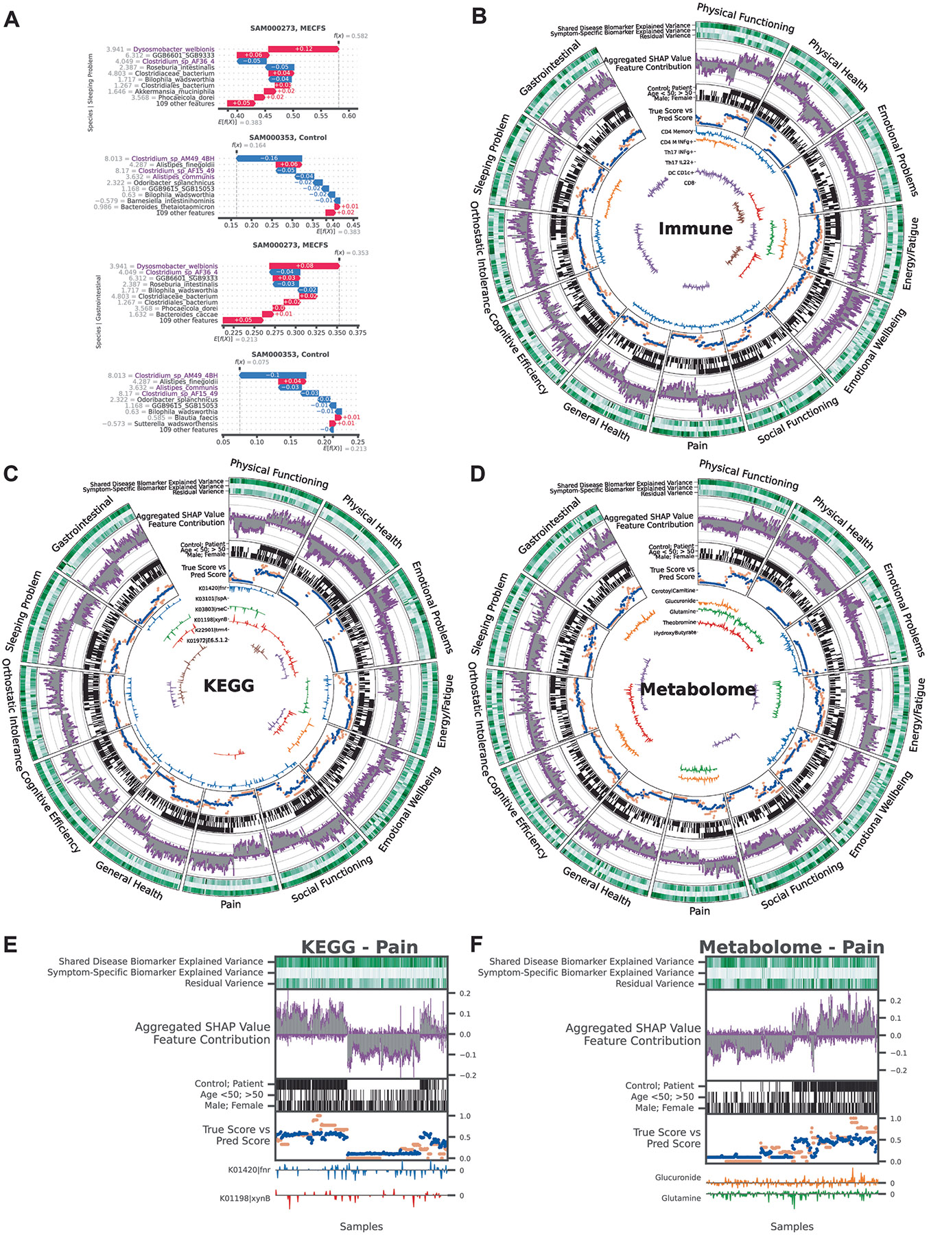
By linking omics profiles to clinical symptoms, BioMapAI identified unique symptom-specific biomarkers in addition to disease-specific biomarkers (Extended Data Fig. 3). Each omics has a circularized diagram (Fig. 3a, Extended Data Fig. 4b-d) to display how BioMapAI use this omics profile to predict 12 clinical symptoms and to discuss the contribution of disease- and symptom-specific biomarkers. Detailed correlation between symptom-specific biomarkers and their corresponding symptoms is in Extended Data Fig. 5. a, Examples of Sleeping Problem-Specific Species’ and Gastrointestinal-Specific Species’ Contributions. Supplemental information for Fig. 3d, which shows the contribution of pain-specific species. b-d, Circularized Diagram for Immune, KEGG and Metabolome Models. Supplemental information for Fig. 3a, which shows the species model. e-f, Zoomed Segment for Pain in KEGG and Metabolome Model. Supplemental information for Fig. 3b, which shows the zoomed segment for pain in the species and immune models. *Note, the reported biomarkers were calculated using the entire dataset and were not validated on held-out data. Abbreviations and Supporting Materials: Extended Data Fig. 5. Related to: Fig. 3.

Extended Data Fig. 5 ∣. Symptom-Specific Biomarkers - Different Correlation Patterns of Biomarkers to Symptom.

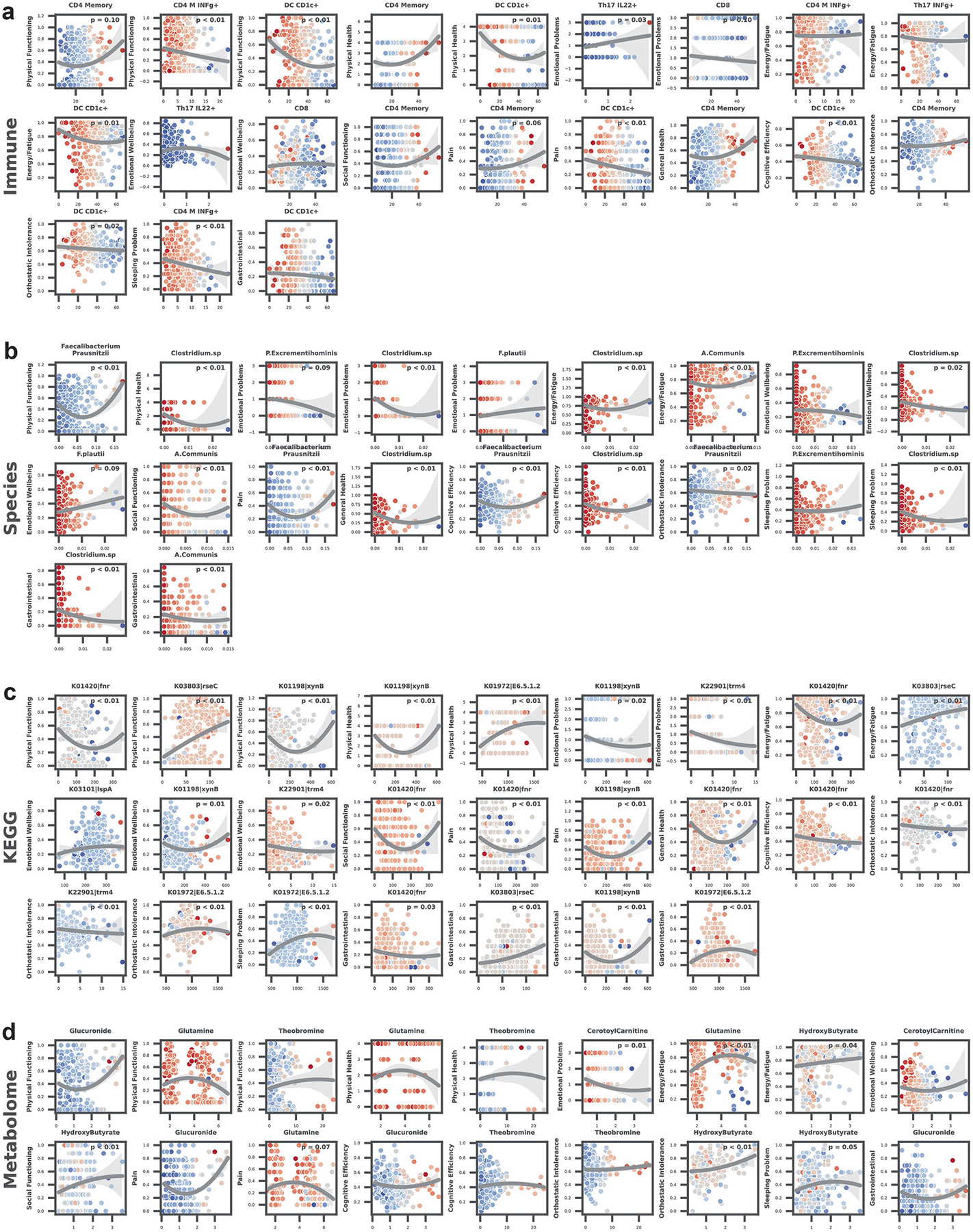
Supplemental information for Fig. 3c, which shows six pain biomarkers from multiple models. Here for each omics (a-d, Immune, Species, KEGG, Metabolome), we plotted the correlation of symptom-specific biomarkers (x-axis) to its related symptom (y-axis), colored by SHAP value (contribution to the symptom). P value by two-sided spearman correlation, FDR adjusted (Detailed statistics in Supplementary Table 5). Abbreviations: CD4, Cluster of Differentiation 4; CD8, Cluster of Differentiation 8; IFNg, Interferon Gamma; DC, Dendritic Cells; MAIT, Mucosal-Associated Invariant T; Th17, T helper 17 cells; CD4+ TCM, CD4+ Central Memory T cells; DC CD1c+ mBtp+, Dendritic Cells expressing CD1c+ and myelin basic protein; DC CD1c+ mHsp, Dendritic Cells expressing CD1c+ and heat shock protein; CD4+ TEM, CD4+ Effector Memory T cells; CD4+ Th17 rfx4+, CD4+ T helper 17 cells expressing RFX4; F. prausnitzii, Faecalibacterium prausnitzii; A. communis, Akkermansia communis; NAD, Nicotinamide Adenine Dinucleotide. Related to: Fig. 3.

Extended Data Fig. 6 ∣. omics WGCNA Modules and Host-Microbiome Network.

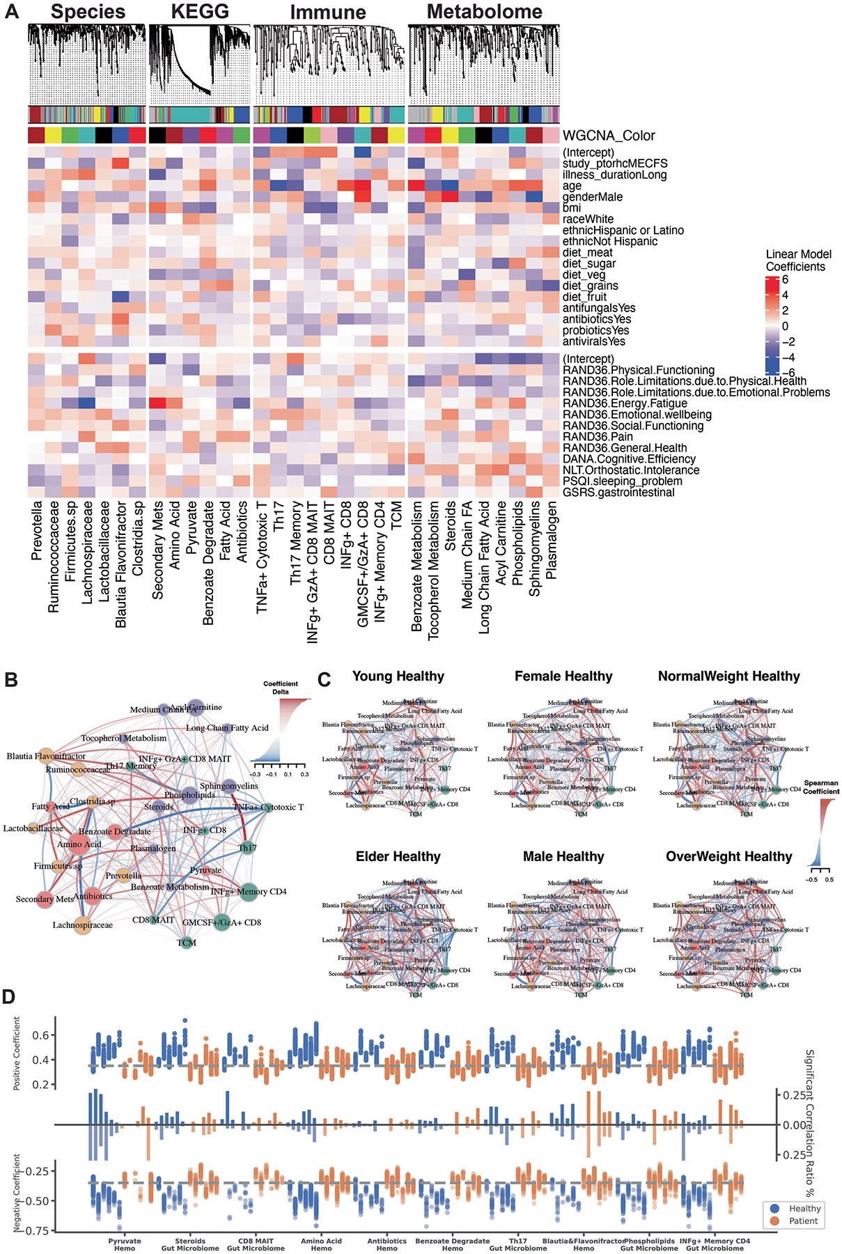
a, Correlation of WGCNA Modules with Clinical Metadata. Weighted Gene Co-expression Network Analysis (WGCNA) was used to identify co-expression modules for each omics layer: species, KEGG, immune, and metabolome. The top dendrograms show hierarchical clustering of ‘omics features, with modules identified. The bottom heatmap shows the relationship of module eigengenes (colored as per dendrogram) with clinical metadata – including demographic information and environmental factors - and 12 clinical scores. General linear models were used to determine the primary clinical drivers for each module, with the color gradient representing the coefficients (red = positive, blue = negative). Microbial modules were influenced by disease presence and energy-fatigue levels, while metabolome and immune modules correlated with age and gender. b-c, Microbiome-Immune-Metabolome Network in b, Patient and c, Healthy Subgroups. Supplemental information for Fig. 4a (Healthy Network) and 4b (Patient Subgroups). Figure 4a is the healthy network; here, Extended Data Fig. 6b presented the shifted correlations in all patients. Figure 4b represented the network in patient subgroups; here, Extended Data Fig. 6c is the corresponding healthy counterpart, for example, female patients were compared with female controls to exclude gender influences. d, Differences in Host-Microbiome Correlations between Healthy and Patient Subgroups. Selected host–microbiome module pairs are grouped on the x-axis (for example, pyruvate to blood modules, steroids to gut microbiome). Significant positive and negative correlations (top and bottom y-axis) of module members pairs are shown as dots for each subgroup (blue = healthy, orange = patient) (Spearman, adjusted p < 0.05), from left to right: Young, Elder, Female, Male, NormalWeight, OverWeight Healthy and Young, Elder, Female, Male, NormalWeight, OverWeight Patient. The middle bars represent the total count of associations. This panel highlights the shifts in host–microbiome networks from health to disease, for example, in patients, the loss of pyruvate to host blood modules correlation and the increase of INFg+ CD4 memory correlation with gut microbiome. Related to: Fig. 4.

Supplementary Material

Supplementary information The online version contains supplementary material available at https://doi.org/10.1038/s41591-025-03788-3.

Data availability

All individual-level data supporting the findings of this study are publicly available. The complete dataset used in this study, including clinical metadata (including demographic information), immune profiles, plasma metabolomics, Quest Diagnostics blood measurements, and processed microbiome data, is available on GitHub: https://github.com/ohlab/BioMapAI/blob/main/data/Omics_Dataset.zip. Raw gut metagenomic sequencing data have been deposited in BioProject: https://www.ncbi.nlm.nih.gov/bioproject/PRJNA1125469.

Code availability

BioMapAI framework and user guide is available at https://github.com/ohlab/BioMapAI. All original code, processed data and trained model of this study has been deposited at Github.

References

- 1.Ruiz-Pablos M, Paiva B, Montero-Mateo R, Garcia N & Zabaleta A. Epstein-Barr virus and the origin of myalgic encephalomyelitis or chronic fatigue syndrome. Front. Immunol 12, 656797 (2021). [DOI] [PMC free article] [PubMed] [Google Scholar]
- 2.Su R. et al. The TLR3/IRF1/type III IFN axis facilitates antiviral responses against enterovirus infections in the intestine. mBio 11, e02540–20 (2020). [DOI] [PMC free article] [PubMed] [Google Scholar]
- 3.Anderson DE et al. Lack of cross-neutralization by SARS patient sera towards SARS-CoV-2. Emerg Microbes Infect. 9, 900–902 (2020). [DOI] [PMC free article] [PubMed] [Google Scholar]
- 4.Cairns R & Hotopf M. A systematic review describing the prognosis of chronic fatigue syndrome. Occup. Med. Oxf. Engl 55, 20–31 (2005). [Google Scholar]
- 5.Cortes Rivera M, Mastronardi C, Silva-Aldana CT, Arcos-Burgos M & Lidbury BA Myalgic encephalomyelitis/chronic fatigue syndrome: a comprehensive review. Diagnostics 9, 91 (2019). [DOI] [PMC free article] [PubMed] [Google Scholar]
- 6.Hare PJ, LaGree TJ, Byrd BA, DeMarco AM & Mok WWK Single-cell technologies to study phenotypic heterogeneity and bacterial persisters. Microorganisms 9, 2277 (2021). [DOI] [PMC free article] [PubMed] [Google Scholar]
- 7.Zeeshan S, Xiong R, Liang BT & Ahmed Z. 100 years of evolving gene–disease complexities and scientific debutants. Brief. Bioinform 21, 885–905 (2020). [DOI] [PubMed] [Google Scholar]
- 8.Poenaru S, Abdallah SJ, Corrales-Medina V & Cowan J. COVID-19 and post-infectious myalgic encephalomyelitis/chronic fatigue syndrome: a narrative review. Ther. Adv. Infect. Dis 8, 20499361211009385 (2021). [DOI] [PMC free article] [PubMed] [Google Scholar]
- 9.Reuken PA et al. Longterm course of neuropsychological symptoms and ME/CFS after SARS-CoV-2-infection: a prospective registry study. Eur. Arch. Psychiatry Clin. Neurosci 274, 1903–1910 (2024). [DOI] [PMC free article] [PubMed] [Google Scholar]
- 10.Bretherick AD et al. Typing myalgic encephalomyelitis by infection at onset: a DecodeME study. NIHR Open Res. 3, 20 (2023). [DOI] [PMC free article] [PubMed] [Google Scholar]
- 11.Bae J & Lin J-MS Healthcare utilization in myalgic encephalomyelitis/chronic fatigue syndrome (ME/CFS): analysis of US ambulatory healthcare data, 2000–2009. Front. Pediatr 7, 185 (2019). [DOI] [PMC free article] [PubMed] [Google Scholar]
- 12.Zheng Y & Zhu Z. Editorial: retrieving meaningful patterns from big biomedical data with machine learning approaches. Front. Genet 14, 1177996 (2023). [DOI] [PMC free article] [PubMed] [Google Scholar]
- 13.Leelatian N. et al. Unsupervised machine learning reveals risk stratifying glioblastoma tumor cells. eLife 9, e56879 (2020). [DOI] [PMC free article] [PubMed] [Google Scholar]
- 14.Su Q. et al. The gut microbiome associates with phenotypic manifestations of post-acute COVID-19 syndrome. Cell Host Microbe 32, 651–660 (2024). [DOI] [PubMed] [Google Scholar]
- 15.Bourgonje AR, van Goor H, Faber KN & Dijkstra G. Clinical value of multiomics-based biomarker signatures in inflammatory bowel diseases: challenges and opportunities. Clin. Transl. Gastroenterol 14, e00579 (2023). [DOI] [PMC free article] [PubMed] [Google Scholar]
- 16.Marcos-Zambrano LJ et al. Applications of machine learning in human microbiome studies: a review on feature selection, biomarker identification, disease prediction and treatment. Front. Microbiol 12, 634511 (2021). [DOI] [PMC free article] [PubMed] [Google Scholar]
- 17.Guo C. et al. Deficient butyrate-producing capacity in the gut microbiome is associated with bacterial network disturbances and fatigue symptoms in ME/CFS. Cell Host Microbe 31, 288–304 (2023). [DOI] [PMC free article] [PubMed] [Google Scholar]
- 18.Raijmakers RPH et al. Multi-omics examination of Q fever fatigue syndrome identifies similarities with chronic fatigue syndrome. J. Transl. Med 18, 448 (2020). [DOI] [PMC free article] [PubMed] [Google Scholar]
- 19.Germain A. et al. Plasma metabolomics reveals disrupted response and recovery following maximal exercise in myalgic encephalomyelitis/chronic fatigue syndrome. JCI Insight 7, e157621 (2023). [Google Scholar]
- 20.Che X. et al. Metabolomic evidence for peroxisomal dysfunction in myalgic encephalomyelitis/chronic fatigue syndrome. Int. J. Mol. Sci 23, 7906 (2022). [DOI] [PMC free article] [PubMed] [Google Scholar]
- 21.Liñares-Blanco J, Fernandez-Lozano C, Seoane JA & López-Campos G. Machine learning based microbiome signature to predict inflammatory bowel disease subtypes. Front. Microbiol 13, 872671 (2022). [DOI] [PMC free article] [PubMed] [Google Scholar]
- 22.He F. et al. Development and external validation of machine learning models for diabetic microvascular complications: cross-sectional study with metabolites. J. Med. Internet Res 26, e41065 (2024). [DOI] [PMC free article] [PubMed] [Google Scholar]
- 23.Mora-Ortiz M, Trichard M, Oregioni A & Claus SP Thanatometabolomics: introducing NMR-based metabolomics to identify metabolic biomarkers of the time of death. Metabolomics 15, 37 (2019). [DOI] [PMC free article] [PubMed] [Google Scholar]
- 24.Balasubramanian R. et al. Metabolomic profiles associated with all-cause mortality in the Women’s Health Initiative. Int. J. Epidemiol 49, 289–300 (2020). [DOI] [PMC free article] [PubMed] [Google Scholar]
- 25.Li H, Ren M & Li Q. 1H NMR-based metabolomics reveals the intrinsic interaction of age, plasma signature metabolites, and nutrient intake in the longevity population in Guangxi, China. Nutrients 14, 2539 (2022). [DOI] [PMC free article] [PubMed] [Google Scholar]
- 26.Kondoh H & Kameda M. Metabolites in aging and aging-relevant diseases: frailty, sarcopenia and cognitive decline. Geriatr. Gerontol. Int 24, 44–48 (2024). [DOI] [PMC free article] [PubMed] [Google Scholar]
- 27.Peng S, Shen Y, Wang M & Zhang J. Serum and CSF metabolites in stroke-free patients are associated with vascular risk factors and cognitive performance. Front. Aging Neurosci 12, 193 (2020). [DOI] [PMC free article] [PubMed] [Google Scholar]
- 28.Duerler P, Vollenweider FX & Preller KH A neurobiological perspective on social influence: serotonin and social adaptation. J. Neurochem 162, 60–79 (2022). [DOI] [PMC free article] [PubMed] [Google Scholar]
- 29.Pomrenze MB, Paliarin F & Maiya R. Friend of the Devil: negative social influences driving substance use disorders. Front. Behav. Neurosci 16, 836996 (2022). [DOI] [PMC free article] [PubMed] [Google Scholar]
- 30.Laslett A-M Empirical and conceptual paradigms for studying secondary impacts of a person’s substance use. Addiction 117, 3148–3149 (2022). [DOI] [PMC free article] [PubMed] [Google Scholar]
- 31.Carco C. et al. Increasing evidence that irritable bowel syndrome and functional gastrointestinal disorders have a microbial pathogenesis. Front. Cell. Infect. Microbiol 10, 468 (2020). [DOI] [PMC free article] [PubMed] [Google Scholar]
- 32.Saffouri GB et al. Small intestinal microbial dysbiosis underlies symptoms associated with functional gastrointestinal disorders. Nat. Commun 10, 2012 (2019). [DOI] [PMC free article] [PubMed] [Google Scholar]
- 33.Liang S, Wu X, Hu X, Wang T & Jin F. Recognizing depression from the microbiota–gut–brain axis. Int. J. Mol. Sci 19, 1592 (2018). [DOI] [PMC free article] [PubMed] [Google Scholar]
- 34.Zhu F, Tu H & Chen T. The microbiota–gut–brain axis in depression: the potential pathophysiological mechanisms and microbiota combined antidepression effect. Nutrients 14, 2081 (2022). [DOI] [PMC free article] [PubMed] [Google Scholar]
- 35.Topan R & Scott SM Sleep: an overlooked lifestyle factor in disorders of gut-brain interaction. Curr. Treat. Options Gastroenterol 21, 435–446 (2023). [Google Scholar]
- 36.Moens de Hase E. et al. Impact of metformin and Dysosmobacter welbionis on diet-induced obesity and diabetes: from clinical observation to preclinical intervention. Diabetologia 67, 333–345 (2024). [DOI] [PMC free article] [PubMed] [Google Scholar]
- 37.Amabebe E, Robert FO, Agbalalah T & Orubu ESF Microbial dysbiosis-induced obesity: role of gut microbiota in homoeostasis of energy metabolism. Br. J. Nutr 123, 1127–1137 (2020). [DOI] [PubMed] [Google Scholar]
- 38.Kavanagh P. et al. Tentative identification of the phase I and II metabolites of two synthetic cathinones, MDPHP and α-PBP, in human urine. Drug Test. Anal 12, 1442–1451 (2020). [DOI] [PubMed] [Google Scholar]
- 39.Lenoir M. et al. Butyrate mediates anti-inflammatory effects of Faecalibacterium prausnitzii in intestinal epithelial cells through Dact3. Gut Microbes 12, 1–16 (2020). [Google Scholar]
- 40.Sokol H. et al. Faecalibacterium prausnitzii is an anti-inflammatory commensal bacterium identified by gut microbiota analysis of Crohn disease patients. Proc. Natl Acad. Sci 105, 16731–16736 (2008). [DOI] [PMC free article] [PubMed] [Google Scholar]
- 41.Monteiro CRAV et al. In vitro antimicrobial activity and probiotic potential of Bifidobacterium and Lactobacillus against species of Clostridium. Nutrients 11, 448 (2019). [DOI] [PMC free article] [PubMed] [Google Scholar]
- 42.Nguyen-Lefebvre AT, Selzner N, Wrana JL & Bhat M. The hippo pathway: a master regulator of liver metabolism, regeneration, and disease. FASEB J. 35, e21570 (2021). [DOI] [PubMed] [Google Scholar]
- 43.Kim C-S Roles of diet-associated gut microbial metabolites on brain health: cell-to-cell interactions between gut bacteria and the central nervous system. Adv. Nutr 15, 100136 (2024). [DOI] [PMC free article] [PubMed] [Google Scholar]
- 44.Rebeaud J, Peter B & Pot C. How microbiota-derived metabolites link the gut to the brain during neuroinflammation. Int. J. Mol. Sci 23, 10128 (2022). [DOI] [PMC free article] [PubMed] [Google Scholar]
- 45.Ahmad S. et al. Gut microbiome-related metabolites in plasma are associated with general cognition. Alzheimers Dement. 17, e056142 (2021). [Google Scholar]
- 46.Ahmed Z, Zeeshan S, Xiong R & Liang BT Debutant iOS app and gene-disease complexities in clinical genomics and precision medicine. Clin. Transl. Med 8, e26 (2019). [Google Scholar]
- 47.Xiong R. et al. Multi-omics of gut microbiome-host interactions in short- and long-term myalgic encephalomyelitis/chronic fatigue syndrome patients. Cell Host Microbe 31, 273–287 (2023). [DOI] [PMC free article] [PubMed] [Google Scholar]
- 48.Sweetman E. et al. Current research provides insight into the biological basis and diagnostic potential for myalgic encephalomyelitis/chronic fatigue syndrome (ME/CFS). Diagnostics 9, 73 (2019). [DOI] [PMC free article] [PubMed] [Google Scholar]
- 49.Hamine S, Gerth-Guyette E, Faulx D, Green BB & Ginsburg AS Impact of health chronic disease management on treatment adherence and patient outcomes: a systematic review. J. Med. Internet Res 17, e3951 (2015). [Google Scholar]
- 50.Derman ID et al. High-throughput bioprinting of the nasal epithelium using patient-derived nasal epithelial cells. Biofabrication 15, 044103 (2023). [Google Scholar]
- 51.Fleming E. et al. Cultivation of common bacterial species and strains from human skin, oral, and gut microbiota. BMC Microbiol. 21, 278 (2021). [DOI] [PMC free article] [PubMed] [Google Scholar]
- 52.Trivedi MS et al. Identification of myalgic encephalomyelitis/chronic fatigue syndrome-associated DNA methylation patterns. PLoS ONE 13, e0201066 (2018). [DOI] [PMC free article] [PubMed] [Google Scholar]
- 53.Bouquet J. et al. Whole blood human transcriptome and virome analysis of ME/CFS patients experiencing post-exertional malaise following cardiopulmonary exercise testing. PLoS ONE 14, e0212193 (2019). [DOI] [PMC free article] [PubMed] [Google Scholar]
- 54.Caruana EJ, Roman M, Hernández-Sánchez J & Solli P. Longitudinal studies. J. Thorac. Dis 7, E537–E540 (2015). [DOI] [PMC free article] [PubMed] [Google Scholar]
- 55.Aurora C, Cecilia A & Adina H. The role of diet in the treatment of chronic diseases case study. ARS Med. Tomitana 27, 153–156 (2021). [Google Scholar]
- 56.Therrien R & Doyle S. Role of training data variability on classifier performance and generalizability. In Medical Imaging 2018: Digital Pathology Vol. 10581, 58–70 (SPIE, 2018). [Google Scholar]
- 57.Krumina A. et al. Clinical profile and aspects of differential diagnosis in patients with ME/CFS from Latvia. Med. (Mex.) 57, 958 (2021). [Google Scholar]
- 58.Zubcevik N. et al. Symptom clusters and functional impairment in individuals treated for Lyme borreliosis. Front. Med 7, 464 (2020). [Google Scholar]
- 59.Lathan C, Spira JL, Bleiberg J, Vice J & Tsao JW Defense automated neurobehavioral assessment (DANA)-psychometric properties of a new field-deployable neurocognitive assessment tool. Mil. Med 178, 365–371 (2013). [DOI] [PubMed] [Google Scholar]
- 60.Resnick HE & Lathan CE From battlefield to home: a mobile platform for assessing brain health. mHealth 2, 30 (2016). [DOI] [PMC free article] [PubMed] [Google Scholar]
- 61.Lee J. et al. Hemodynamics during the 10-minute NASA Lean Test: evidence of circulatory decompensation in a subset of ME/CFS patients. J. Transl. Med 18, 314 (2020). [DOI] [PMC free article] [PubMed] [Google Scholar]
- 62.Committee on the Diagnostic Criteria for Myalgic Encephalomyelitis/ChronicFatigue Syndrome, Board on the Health of Select Populations, & Institute of Medicine. Beyond Myalgic Encephalomyelitis/Chronic Fatigue Syndrome: Redefining an Illness (National Academies Press, 2015). [Google Scholar]
- 63.36-Item Short Form Survey (SF-36) Scoring Instructions. RAND Health Care https://www.rand.org/health-care/surveys_tools/mos/36-item-short-form/scoring.html (1992).
- 64.Blanco-Míguez A. et al. Extending and improving metagenomic taxonomic profiling with uncharacterized species using MetaPhlAn 4. Nat. Biotechnol 41, 1633–1644 (2023). [DOI] [PMC free article] [PubMed] [Google Scholar]
- 65.Edgar RC Search and clustering orders of magnitude faster than BLAST. Bioinformatics 26, 2460–2461 (2010). [DOI] [PubMed] [Google Scholar]
- 66.Love MI, Huber W & Anders S. Moderated estimation of fold change and dispersion for RNA-seq data with DESeq2. Genome Biol. 15, 550 (2014). [DOI] [PMC free article] [PubMed] [Google Scholar]
- 67.Saripuddin M, Suliman A, Syarmila Sameon S & Jorgensen BN Random undersampling on imbalance time series data for anomaly detection. In Proc. 2021 4th International Conference on Machine Learning and Machine Intelligence 151–156 (Association for Computing Machinery, 2022). [Google Scholar]
- 68.Lundberg S & Lee S-I A Unified approach to interpreting model predictions. Preprint at 10.48550/arXiv.1705.07874 (2017). [DOI] [Google Scholar]
- 69.Friedman JH, Hastie T & Tibshirani R. Regularization paths for generalized linear nodels via coordinate descent. J. Stat. Softw 33, 1–22 (2010). [PMC free article] [PubMed] [Google Scholar]
- 70.Kuhn M. Building predictive models in R using the caret package. J. Stat. Softw 28, 1–26 (2008). [DOI] [PMC free article] [PubMed] [Google Scholar]
- 71.Langfelder P & Horvath S. WGCNA: an R package for weighted correlation network analysis. BMC Bioinformatics 9, 559 (2008). [DOI] [PMC free article] [PubMed] [Google Scholar]
- 72.Antonov M, et al. igraph enables fast and robust network analysis across programming languages. Preprint at 10.48550/arXiv.2311.10260 (2023). [DOI] [Google Scholar]
- 73.Koo TK & Li MY A guideline of selecting and reporting intraclass correlation coefficients for reliability research. J. Chiropr. Med 15, 155–163 (2016). [DOI] [PMC free article] [PubMed] [Google Scholar]
- 74.Nelder JA & Wedderburn RWM Generalized linear models. J. R. Stat. Soc. Ser. Gen 135, 370–384 (1972). [Google Scholar]
- 75.Bakdash JZ & Marusich LR Repeated measures correlation. Front. Psychol 8, 456 (2017). [DOI] [PMC free article] [PubMed] [Google Scholar]
- 76.Gu C. Smoothing Spline ANOVA Models: R Package gss (Springer, 2013). [Google Scholar]
Associated Data
This section collects any data citations, data availability statements, or supplementary materials included in this article.
Supplementary Materials
Data Availability Statement