Inverting dynamic force microscopy: From signals to time-resolved interaction forces

Abstract

Transient forces between nanoscale objects on surfaces govern friction, viscous flow, and plastic deformation, occur during manipulation of matter, or mediate the local wetting behavior of thin films. To resolve transient forces on the (sub) microsecond time and nanometer length scale, dynamic atomic force microscopy (AFM) offers largely unexploited potential. Full spectral analysis of the AFM signal completes dynamic AFM. Inverting the signal formation process, we measure the time course of the force effective at the sensing tip. This approach yields rich insight into processes at the tip and dispenses with a priori assumptions about the interaction, as it relies solely on measured data. Force measurements on silicon under ambient conditions demonstrate the distinct signature of the interaction and reveal that peak forces exceeding 200 nN are applied to the sample in a typical imaging situation. These forces are 2 orders of magnitude higher than those in covalent bonds.

Time-dependent forces mediate adsorption, ordering phenomena, and visco-elasticity that are important in rheology and tribology, as well as in biology and catalysis. The importance of dynamic aspects becomes obvious when looking at the viscoelastic properties of polymers (1, 2). Even on the level of a single biomolecule under external stress, velocity dependence can be observed: the stability of the molecule increases with the applied force rate (3). However, dynamic forces occurring during processes at surfaces, in thin and confined lubrication films, or on the level of nanoscopic objects are experimentally not easily accessible.

In this context, atomic force microscopy (AFM) offers a large potential to investigate and manipulate material at the (sub) microsecond time scales and nanometer length scale. AFM (4) and related techniques (5) have gained increasing importance in many fields of research and industrial applications. Raster scanning the sample with a sharp tip attached to the end of the microfabricated cantilever allows not only the visualization of objects in shape and size of single molecules, but also the ability to touch and squeeze, pull and push them (6). In dynamic force microscopy, the motion of the cantilever is externally modulated. In tapping-mode AFM, the most common dynamic mode, the cantilever is excited to oscillate at its fundamental resonant frequency. Once each oscillation cycle, the tip interacts with the surface, and information about the tip-sample interaction is transferred into the time course of the signal. The signal formation process is depicted in Fig. 1, and the inset shows schematically the setup of tapping-mode AFM.

Figure 1.

The flow diagram represents dynamic AFM, the setup is sketched in the Inset. Conceiving the AFM as sensor, it converts the force input f(x, t) into the signal output s(x, x′, t) in a linear manner (upper branch; t time, x position of the acting force, x′ position of measurement). The interaction between tip and sample obeys a nonlinear force-distance relation (lower, back-coupled branch). Physically, the cantilever is externally excited to oscillate and interacts once every cycle with the sample that is mounted on a scan-piezo. The deflection of the cantilever is measured by a laser, reflected from the backside of the cantilever onto a position-sensitive photodiode.

To obtain the acting forces from the dynamics of the oscillating cantilever, there are basically two routes. First, under ultra high vacuum conditions, the change of the resonant frequency of the force-coupled cantilever is used to estimate the interaction potential (7–9). These methods highly depend on the high quality factor of the oscillation under ultra high vacuum. Second, under ambient conditions, the tip-sample interaction is commonly estimated under the assumption of a disturbed harmonic oscillation using contact mechanical models where the choice of the “best model” is crucial (10–15). These approaches are based mostly on forward simulations requiring vast a priori knowledge about the interaction. Approximations are inevitable for systems of complex materials such as polymers, layered material, or biological specimens. Dynamic effects such as viscous flow, capillary formation, or the rearrangement of surface charges provide a further challenge.

Complementary to the forward simulation of the cantilever motion, we present a backward signal analysis approach to determine the force directly from the measured signal. It is exactly the information in anharmonic signal contributions that encodes the duration and the strength of the interaction (16–22): the nonlinear interaction generates higher harmonics of the fundamental oscillation, resonantly enhanced to significant signal contributions by higher eigenmode excitation. To measure the full time course of the interaction force at the sensing tip we decode this information by inverting the signal formation process. Thus, the effective force at the tip during each single tip-sample interaction event is entirely reconstructed from measured data without a priori assumptions concerning acting forces. We present time-resolved and quantitative data on the interaction forces in a typical tapping-mode AFM experiment under ambient conditions.

Theoretical Considerations

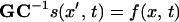
Conceiving the AFM as a sensor, information about the tip-sample interaction is transferred into the deflection signal as sketched in the flow diagram of Fig. 1. The force distribution f(x, t), with position x along the cantilever and time t, acts as input signal into the sensor. This force deflects the cantilever (linear operator G) resulting in the bending shape Ψ(x, t), as described by the equation of motion, GΨ(x, t) = f(x, t). At this point, the flow diagram exhibits two branches as indicated in Fig. 1. The nonlinear circuit (lower part) corresponds to the interaction: Ψ(x, t) determines the tip-sample separation that enters the nonlinear force law of the interaction, and thus couples back on the force distribution f(x, t). In contrast, the measurement of the cantilever motion relies on a second, here linear path, wherein the linear and bijective operator C represents the detection (i.e. the photodiode and the electronics). It converts the bending shape Ψ(x, t) into the signal s(x′, t) according to s(x′, t) = CΨ(x, t). Briefly, the AFM as linear sensor detects nonlinear forces acting at its tip.

For both the operators G and C, linearity¶ is an appropriate assumption in the case of a typical AFM experiment, where cantilever deflections from equilibrium shape remain small, and only waves traveling on the cantilever with wavelengths above 0.1l (with cantilever length l) have to be considered (23). Under these conditions, the linear equation

1

governs signal formation in dynamic AFM. Operator GC⁻¹ maps the time course of the signal into the time course of the force. Especially, one physical value is mapped on exactly one signal value, and vice versa, which is an important requirement for a sensor.

Linearity of the operator GC⁻¹ allows describing dynamic AFM in the framework of linear response theory, e.g., ref. 26. For calculation, an appropriate and complete set of orthogonal functions is chosen to describe both the linear operator GC⁻¹ and the functions. In Fourier space, the complex-valued and dimensionless transfer function T(x, x′, ω) is one representation of the inverse of operator GC⁻¹. Here, the description in Fourier space seems favorable because it is well adapted to the problem and leads to a concise formalism. This choice does not imply that only repetitive processes can be analyzed, and other choices are possible, e.g., the Laplace transform (26, 27). Notably, allowed force distributions at the input include Dirac's delta distribution δ(⋅), defined by g(χ) = ∫δ(χ − χ′)g(χ′)dχ′, where χ takes the role of time t or position x. Indeed, T(x, x′, ω) is defined to be the response of the system to F(ω) = 1 for all ω, which is the Fourier transform of the delta distribution.

Given a certain force distribution as input, the response of the AFM to that force is given by

2

Here, l denotes the length of the cantilever, ω the angular frequency, and capital letters indicate Fourier-transformed quantities (signal S and force F). In the notation of Eq. 2, the transfer function is normalized to the static case, i.e. ∥T(x, x′, ω = 0)∥ = 1, and the scaling coefficient u carries the dimensions.

Usually, the deflection is measured at one fixed position only, i.e. S(ω) = S(x′ = x_laser, ω), and the force acting right at the tip clearly dominates the force distribution,‖ i.e., F(x, ω) ≈ F(x = x_tip, ω) := F(ω). Thus, the reduced transfer function T(ω) = T(x = x_tip, x′ = x_laser, ω) suffices to calculate the force at x_tip from

3

For Eq. 3 to hold, T(ω) must be a single-valued function with ∥T(ω)∥ > 0 for all frequencies: the process of measurement must neither erase information nor render it ambiguous. In the outlined analysis, the signal is subjected to a linear transformation, defined by the transfer function. No information contained in the signal is rejected, and no approximation is applied to the signal. In practice, noise degrades information about the time course of the force, and the analysis has to exclude frequency bands with unreliable information. Critical frequency bands are those with ∥T(ω)∥ ≪ 1 and strongly depend on the type of cantilever used. In these frequency bands, signal contributions can fall below the effective noise level introduced by the detection electronics. A further important issue is the question of negligibility of small signal contributions. In frequency bands with ∥T(ω)∥ ≪ 1, the signal amplitude at a higher harmonic can be small compared to the signal at the fundamental frequency, but the corresponding information content can be important. This becomes clear considering an input F(ω) ≡ 1 for all ω, where the response equals T(ω): Even though this input possesses homogeneous information content over all frequencies, the maximal and minimal signal contributions will differ by several orders of magnitude according to T(ω). Thus, the mere “smallness” of a signal contribution does not justify its neglection.

To reconstruct the time course of the force from the time series of the deflection signal obtained in the experiment, knowledge of the transfer function T(ω) is essential. Inversion of Eq. 3 defines a measurement procedure, where a well-defined force input F̂(ω) containing all frequencies is exerted on the tip of the free cantilever. From the recorded response Ŝ(ω), the transfer function is calculated by T(ω) = Ŝ(ω)/F̂(ω).

Materials and Methods

Experimental Details.

A Nanoscope Multimode IIIa (Veeco/Digital Instruments, Santa Barbara, CA) was used with external amplification of the deflection signal (SR560, Stanford Research, Sunnyvale, CA) that was recorded at 5 M sample/s (NI PCI-6110E, National Instruments, Austin, TX). The spring constant 3.8 ± 0.4 N/m of the v-shaped Si-cantilever (200 μm length; type NSCH 11, Silicon-MDT, Moscow) was determined by standard thermal-noise calibration (28). The two samples investigated were: silicon (100) waver with natural oxide layer (Wacker Chemie, Burghausen, Germany), and polytetrafluoroethylene (PTFE) foil (GM Gummi and Kunststoffe, Munich), glued to a sample mount. Both samples were cleaned with ethanol and ultrapure water before use. The transfer function was calculated on the basis of the average of 87 rupture events, with imaginary and real parts locally smoothed by cubic functions. The reconstruction used a sliding Fourier transform algorithm. In a first step, a subset of 32,768 data points was extracted from the full time series of 448,668 data points by using a windowing function with Gaussian flanks. In the second step, the subset was Fourier-transformed. Contributions ∥S(ω)∥ ≥ ∥3L(ω)∥ were identified as signal, and a steep weight function [5% at 2L(ω)] suppressed frequency ranges with unreliable information content. Here, L(ω) denotes the noise level, estimated from the Fourier spectrum (see Fig. 2B) excluding the harmonics, in which the periodic signal is concentrated. Eq. 3 was applied, and an additional low-pass filter with Gaussian flank limited the bandwidth to 733 kHz accounting for uncertainties in the transfer function. In the third step, the subset was retransformed into the time domain. The resulting curve represents force vs time. To minimize boundary effects, the impact event in the middle of the curve was extracted corresponding to one tapping cycle (i.e., ∼108 data points). For iterating the procedure, the initial windowing function was shifted by one tapping cycle. Finally, the full curve force vs time was composed from the extracted events avoiding overlap. This algorithm ensures that each single impact event is addressed while boundary effects are minimized.

Figure 2.

In the framework of linear response theory, the conversion of input into output is described by the transfer function of the AFM. (A) The transfer function was measured for the used configuration with a bandwidth of 1.2 MHz. Eigenmode resonances of this multimodal resonator are indicated. (B) The depicted amplitude spectrum of the signal (normalized to the free oscillation) was obtained on silicon at an average tip-sample separation corresponding to 44.6% of the free amplitude. The periodic contact of the AFM tip with the silicon sample introduces higher harmonics that couple to the eigenmode resonances. In general, eigenmodes resonances are not harmonics of the fundamental oscillation. Note the noise level.

Single-Degree-of-Freedom Simulation.

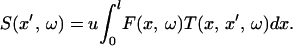
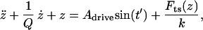
The cantilever is described as an impacting harmonic oscillator, where the tip-sample contact was modeled (R.W.S., unpublished work) in a well-established Derjaguin–Müller–Toporov (DMT) approach, following ref. 15. With the transformation t′ = tω₁, the equation of motion is given by

4

with the DMT tip-sample force

5

where z is the position. All parameters are denoted and their values are listed in Table 1. The simulation was implemented with MATLAB R12 (Mathworks, Natick, MA) using simulink. The simulations were integrated with ode23s, which is an implementation of an explicit Runge–Kutta (2,3) pair of Bogacki and Shampine.

Table 1.

Parameters used for the simulation

Quality factor	Q = 30
Free vibration amplitude	A0 = 45 nm
Resonant frequency	ω0 = 2π 46.2 kHz
Spring constant	k = 3.8 N/m
Tip radius	R = 30 nm
Drive amplitude	Ad = A0/Q
Drive frequency	ωd = ω0
Dimensionless time	t′ = t ω0 × 103
Elastic moduli (Si)	Et = Es = 169 GPa
Poisson number (Si)	νt = νs = 0.28 GPa
Hamaker constant (SiO2)	H = 6.4⋅10−11 nJ
Surface energy (SiO2)	γ = 0.031 J·m−2
Interatomic distance	a0 =

The elastic behavior of tip and sample is modeled by the values for bulk-silicon, whereas the values for SiO₂ are used for the surface energy and the Hamaker constant modeling the natural oxide layer. 

Measuring the Transfer Function

Measuring the transfer function is crucial to describe the actual situation. Otherwise, assumptions are necessary about the specific cantilever, the current adjustment of the deflection readout, and the setting of the electronics, so the reconstructed forces become unreliable. Here, we measured the transfer function in the last step of the whole experiment, avoiding early damage of the tip. To determine the transfer function, quasi-static force curves (no excitation of the cantilever) were performed on double-sided adhesive tape, generating a step function with well-known step height as input on the cantilever. Retracting the cantilever from the surface, the adhesion ruptures, and the tip is released. This rupture event defines the step (330 nN in the case presented). The transfer function derived by this procedure describes the response of the AFM to forces effective right at the tip and the resulting deflection measured at a fixed second position. A background of viscous damping and long-range forces along the cantilever is conceived as internal force of the AFM system and automatically incorporated into the transfer function. Fig. 2A depicts magnitude and phase of the smoothed transfer function of the AFM. Clearly visible are the resonances of the first four eigenmodes of the cantilever at 46.2 kHz, 247 kHz, 581 kHz, and 1,051 kHz. Comparing the transfer function with the signal amplitude spectrum of Fig. 2B, the enhancement of harmonic contributions caused by higher eigenmode excitation becomes evident.

Overview of the Measured Data and Simulation

In our experiment the deflection signal was recorded during tapping mode (i.e., cantilever excitation at its fundamental resonance ω₁ = 2π 46.2 kHz) approach curves on silicon and PTFE under ambient conditions. With the transfer function determined under identical conditions, we finally reconstructed the time course of the force according to Eq. 3.

For the case of silicon, Fig. 3 summarizes important aspects of the approach curve in dependence of the piezo displacement. For orientation, the amplitude A₁ at ω₁ is given in Fig. 3E. It decreases linearly with decreasing mean tip-sample distance. Signal amplitudes at selected frequencies are depicted in Fig. 3A. The fifth harmonic is close to the resonance of the second vertical eigenmode, while the 12th harmonic is associated to eigenmode 3: their appearance proves the excitation of higher eigenmodes upon tip-sample interaction and confirms earlier results (19, 20). Additionally, the amplitude at 0.5 ω₁ marks the regime of period doubling (29). All amplitudes are normalized to the free amplitude (42 nm). Further graphs in Fig. 3 show peak and average forces (f_min, f_max, and 〈f〉, respectively), as well as the average duration of the interaction 〈τ〉 (determined by thresholding at −12 nN) for each tapping cycle. Three distinct regions occur, where peak forces remain almost constant, while transitions become prominent in two further regions, all marked in Fig. 3. Forces are small in the case of the freely oscillating cantilever (up to 41.6 nm piezo displacement). Negative forces mark the onset of attractive interaction. In this regime, the interaction lasts around 7% of the cycle time (22 μs). The onset of contact leads to the appearance of repulsive contributions, and changes in duration and spectral composition of the impact. Above 61 nm piezo displacement, repulsive forces exceed 200 nN and indicate mechanical contact. At the same time, the average force changes to positive values around 2 nN, and the interaction lasts more than 20% of the whole tapping cycle. Period-doubled behavior is embedded in the predominantly repulsive regime.

Figure 3.

Several parameters are shown, characterizing the tapping-mode approach curve on silicon under ambient conditions. (A) Signal amplitudes A₅ and A₁₂ (fifth and 12th harmonic to the fundamental frequency ω₁ = 2π 46.2 kHz, respectively) indicate excitation of vertical eigenmodes 2 and 3, the appearance of contributions at 0.5 ω₁ marks period doubling. (B) Maximal forces f_max reach +200 nN (repulsive force), whereas minimal forces f_min (attractive force) become more pronounced with the onset of mechanical contact (−40 nN to −100 nN). (C) Along with this transition, the force averaged over one cycle 〈f〉 changes sign, but remains within ±2 nN. (D) The average duration of the interaction 〈τ〉 increases from 7% for purely attractive interaction to more than 25% for repulsive dominated interaction. (E) For orientation, the amplitude A₁ at the excitation frequency ω₁ is given. It decreases linearly with decreasing mean tip-sample distance. The distinct regimes and transitions are marked i–v. The arrows point to the positions where the events of Fig. 5A were taken.

To cross-check these results with current models for tapping-mode AFM (11, 12, 30) we performed a single-degree-of-freedom simulation following ref. 15. There, the cantilever is modeled as an impacting harmonic oscillator. Parameters are chosen to match the experimental situation as detailed in Table 1, especially concerning the cantilever used in the experiment. The tip-sample contact is modeled with a Derjaguin–Müller–Toporov approach for a tip of 30 nm radius. The simulated average and maximal forces (Fig. 4) agree reasonably well with the experimental data (Fig. 3). Notably, the simulation reveals peak forces in the range of 200 nN, which occurred also in the measured data.

Figure 4.

Approach curves simulated with a single degree of freedom based on a Derjaguin–Müller–Toporov contact model (with the parameters given in Table 1.) are shown vs. the tip-sample separation. (A) Forces averaged over one cycle reach approximately 2 nN. (B) Maximum and minimum forces (f_max and f_min, respectively) were determined by a peak detection algorithm. While the maximum forces fits reasonable well to the experimental data, the minimum forces (i.e., the attractive forces) deviate remarkably from the experiment: the simulation does not account for the dissipative forces occurring in the experiment. (C) The depicted tapping amplitude A was derived from the peak-to-peak values.

In contrast, the simulated minimum forces (Fig. 4B) differ remarkably from the measurement, because the model completely ignores the influence of dissipative surface forces. Furthermore, the simulation considers only the fundamental mode, and thus cannot account for higher eigenmode excitation. It lacks dynamic surfaces forces and relies on a priori assumptions concerning the set of parameters. Nevertheless, such a model is useful to estimate general aspects of a dynamic AFM experiment.

Time-Resolved Dynamic AFM

Complementary to the simulation, the time-resolved signal analysis outlined before offers detailed insight into the time course of the tip-sample interaction.

Fig. 5A shows force f(t) and signal s(t) of typical impact events; the full time series is available as Movie 1, which is published as supporting information on the PNAS web site, www.pnas.org. Clearly, the impact events reach high peak forces and are strongly concentrated in their time course, leading to small average forces.

Figure 5.

The time course of reconstructed force f(t) and measured signal s(t) (below the force graphs, scale bars indicate the free signal amplitude) are shown for representative impact events, extracted from the positions marked i–v in Fig. 3E. The events are (i) free oscillation, (ii) purely attractive interaction, and (iii) onset of contact. (iv) As the tip enters deeply into the interaction potential, repulsive forces become predominant and exceed +200 nN (note the scale). At the same time, attractive forces increase quite dramatically, and the total duration of the interaction pulse rises to 3.5 μs, confirming earlier results obtained with a different method (19). The impact follows a typical sequence of attractive, repulsive, and again attractive force, just as in the case of a quasi-static force curve. (v) For a certain set of parameters the nonlinearity in the effective external force can result in period doubling, and thus in a characteristic oscillation of the force pattern (note the different time scale). Even in this case, we consider the cantilever itself still a linear sensor. (B) Comparing the impact event obtained on silicon with that on PTFE measured with the identical tip under comparable conditions reveals material dependence (note the different force scales). Whereas a large attractive force precedes the mechanical contact on silicon, the tip touches the PTFE surface almost immediately (see *). This difference in the transient force points to the influence of surface wetting on silicon.

The events depicted in Fig. 5A are taken from the positions marked in Fig. 3E and are representative for the different regimes: (i) free oscillation, (ii) purely attractive interaction, (iii) onset of mechanical contact, (iv) predominantly repulsive interaction, and (v) period doubling. All curves are corrected for the external excitation that resulted in a sinusoidal force with 5 nN amplitude at the tip, as concluded from the case of free oscillation. The limited bandwidth underestimates peak heights and leads to smoothing of fast events. Thus, the reconstructed time course represents a lower limit. Comparing the impact events on silicon and PTFE (excitation reduced to 75% compared to the case of silicon) clearly demonstrates material specificity (Fig. 5B; note the scales). The asymmetry in the case of PTFE is striking (see * in Fig. 5B), and peak forces reach only 25% of those on silicon. This comparison indicates the pronounced influence of surface wetting on silicon by a water film (31–33), leading to attractive forces caused by the formation of a liquid neck between tip and sample during each cycle (34).

The observed signature of the impacts reflects the nonlinear interaction, sampled by the tip in each cycle, similar to quasi-static force curves. Nevertheless, with far more than 100 nN peak force the tip-sample interaction is not gentle, e.g. binding forces in covalent bonds are 2 orders of magnitude smaller (35). Even purely attractive forces reach −40 nN.

To avoid structural breakdown, the impact force has to be distributed over a large number of bonds. For estimation, we assume Hertzian contact mechanics, where the contact area is given by

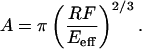6

Here, R denotes the tip radius, F the impact force, and E_eff the effective tip-sample stiffness. The latter parameter describes the material properties of tip and sample. With the respective material parameters (Table 1) the effective tip-sample stiffness is given by

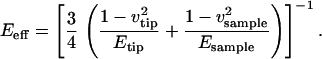7

For a tip of 30 nm radius, an impact force of 200 nN, and with the material parameters given in Table 1, the estimated contact area is 23 nm², i.e., ∼40 unit cells on each side of the contact, and hence ∼640 atoms contribute to the contact.

From this analysis we conclude that the high peak forces occurring in tapping-mode AFM under ambient conditions and in the repulsive force regime limit the resolution in the images. Furthermore, the high forces give evidence for distortion or destruction of sample and tip under typical tapping-mode imaging conditions. This notion was previously inferred indirectly from measured data (destroyed molecules) and single-degree-of-freedom forward calculations (36, 37). On the other hand, the vast number of soft samples successfully imaged under comparable conditions indicates the importance of dynamic aspects such as peak forces and interaction durations.

In the reconstructed force, transient events are clearly visible. On the slow time scale, the continuous decrease of the signal amplitude is reflected in general changes of the reconstructed force. The transitions between the mentioned force regimes as well as the onset of bifurcation occur on the midrange time scale. The onset of mechanical contact especially leads to an abrupt change in the cantilever oscillation (Fig. 3A) and an overshooting average force (Fig. 3C). This overshooting is reproduced in the simulation (Fig. 4A). Notably close to the transitions between the regimes the impact events differ from one to the following, revealing transient events on the fast time scale (Fig. 5A and Movie 1).

The demonstrated spectral analysis introduces dynamic AFM as time-resolving technique and opens the field to locally access transient surface forces. These transient forces are responsible for plastic deformation and are involved in friction and wetting. Using the AFM as nano-manipulator, the analysis presented explains the transition between imaging and cutting thin filaments, such as DNA. The dynamic response of thin polymer films (1, 2), and their wetting behavior on the scales of nanometers and (sub) microseconds becomes accessible. It finds its counterpart in the dynamic stiffness of molecules pulled (3) or squeezed by the AFM tip.

Recent development of fast cantilevers and detection setups will push the accessible resolution of transient forces to nanoseconds and beyond (38). “Pulse shaping” opens a further exciting approach to probe forces on the molecular level: based on the spectral analysis, the dynamic force exerted on the sample can be designed by shaping the probing force pulse through spectrally matched excitation at the cantilever base.

Abbreviations

AFM

atomic force microscopy

PTFE

polytetrafluoroethylene

References

- 1.Ferry J D. Viscoelastic Properties of Polymers. New York: Wiley; 1980. [Google Scholar]
- 2.Wilhelm M. Macromol Mater Eng. 2002;287:83–105. [Google Scholar]
- 3.Evans E, Ritchie K. Biophys J. 1997;72:1541–1555. doi: 10.1016/S0006-3495(97)78802-7. [DOI] [PMC free article] [PubMed] [Google Scholar]
- 4.Binnig G, Quate C F, Gerber C. Phys Rev Lett. 1986;56:930–933. doi: 10.1103/PhysRevLett.56.930. [DOI] [PubMed] [Google Scholar]
- 5.Friedbacher G, Fuchs H. Pure Appl Chem. 1999;71:1337–1357. [Google Scholar]
- 6.Oesterhelt F, Oesterhelt D, Pfeiffer M, Engel A, Gaub H E, Müller D J. Science. 2000;288:143–146. doi: 10.1126/science.288.5463.143. [DOI] [PubMed] [Google Scholar]
- 7.Giessibl F J. Phys Rev B Condens Matter. 1997;56:16010–16015. [Google Scholar]
- 8.Hölscher H, Allers W, Schwarz U D, Schwarz A, Wiesendanger R. Phys Rev Lett. 1999;83:4780–4783. [Google Scholar]
- 9.Lantz M A, Hug H J, Hoffmann R, van Schendel P J A, Kappenberger P, Martin S, Baratoff A, Guntherodt H-J. Science. 2001;291:2580–2583. doi: 10.1126/science.1057824. [DOI] [PubMed] [Google Scholar]
- 10.Sarid D, Ruskell T G, Workman R K, Chen D. J Vacuum Sci Technol B. 1996;14:864–867. [Google Scholar]
- 11.Tamayo J, Garcia R. Langmuir. 1996;12:4430–4435. [Google Scholar]
- 12.Burnham N A, Behrend O P, Oulevey F, Gremaud G, Gallo P-J, Gourdon D, Dupas E, Kulik A J, Pollock H M, Briggs G A D. Nanotechnology. 1997;8:67–75. [Google Scholar]
- 13.Cleveland J P, Anczykowski B, Schmid A E, Elings V B. Appl Phys Lett. 1998;72:2613–2615. [Google Scholar]
- 14.Bielefeldt H, Giessibl F J. Surface Sci Lett. 1999;440:L863–L867. [Google Scholar]
- 15.Garcia R, San Paulo A. Phys Rev B. 2000;61:R13381–R13384. [Google Scholar]
- 16.Franklin W S. Phys Rev. 1894;1:442–450. [Google Scholar]
- 17.Stark R W, Heckl W M. Surface Sci. 2000;457:219–228. [Google Scholar]
- 18.Dürig U. New J. Phys. 2000. http://www.njp.org/2 http://www.njp.org/2, 5.1–5.12. , 5.1–5.12. [Google Scholar]
- 19.Hillenbrand R, Stark M, Guckenberger R. Appl Phys Lett. 2000;76:3478–3480. [Google Scholar]
- 20.Stark M, Stark R W, Heckl W M, Guckenberger R. Appl Phys Lett. 2000;77:3293–3295. [Google Scholar]
- 21.Sahin O, Atalar A. Appl Phys Lett. 2001;79:4455–4457. [Google Scholar]
- 22.Rodriguez T R, Garcia R. Appl Phys Lett. 2002;80:1646–1648. [Google Scholar]
- 23.Clough R W, Penzien J. Dynamics of Structures. New York: McGraw–Hill; 1993. [Google Scholar]
- 24.Turner J A, Hirsekorn S, Rabe U, Arnold W. J Appl Phys. 1997;82:966–979. [Google Scholar]
- 25.Rabe U, Janser K, Arnold W. Rev Sci Instrum. 1996;67:3281–3293. [Google Scholar]
- 26.Carlson G E. Signal and Linear System Analysis. New York: Wiley; 1998. [Google Scholar]
- 27.Unbehauen R. Systemtheorie 1–Allgemeine Grundlagen, Signale und Lineare Systeme im Zeit und Frequenzbereich. Munich: Oldenbourg; 1997. [Google Scholar]
- 28.Stark R W, Drobek T, Heckl W M. Ultramicroscopy. 2001;86:207–215. doi: 10.1016/s0304-3991(00)00077-2. [DOI] [PubMed] [Google Scholar]
- 29.Burnham N A, Kulik A J, Gremaud G, Briggs G A D. Phys Rev Lett. 1995;74:5092–5095. doi: 10.1103/PhysRevLett.74.5092. [DOI] [PubMed] [Google Scholar]
- 30.Hunt J P, Sarid D. Appl Phys Lett. 1998;72:2969–2971. [Google Scholar]
- 31.Israelachvili J N, Pashley R M. Nature (London) 1983;306:249–250. [Google Scholar]
- 32.Raviv U, Laurat P, Klein J. Nature (London) 2001;413:51–54. doi: 10.1038/35092523. [DOI] [PubMed] [Google Scholar]
- 33.Heuberger M, Zäch M, Spencer N D. Science. 2001;292:905–908. doi: 10.1126/science.1058573. [DOI] [PubMed] [Google Scholar]
- 34.Colchero J, Storch A, Luna M, Herrero J G, Baro A M. Langmuir. 1998;14:2230–2234. [Google Scholar]
- 35.Grandbois M, Beyer M, Rief M, Clausen-Schaumann H, Gaub H E. Science. 1999;283:1727–1730. doi: 10.1126/science.283.5408.1727. [DOI] [PubMed] [Google Scholar]
- 36.San Paulo A, García R. Biophys J. 2000;78:1599–1605. doi: 10.1016/S0006-3495(00)76712-9. [DOI] [PMC free article] [PubMed] [Google Scholar]
- 37.Pignataro B, Chi L, Gao S, Anczykowski B, Niemeyer C, Adler M, Fuchs H. Appl Phys A. 2002;74:447–452. [Google Scholar]
- 38.Viani M B, Pietrasanta L I, Thompson J B, Chand A, Gebeshuber I C, Kindt J H, Richter M, Hansma H G, Hansma P K. Nat Struct Biol. 2000;7:644–647. doi: 10.1038/77936. [DOI] [PubMed] [Google Scholar]
Associated Data
This section collects any data citations, data availability statements, or supplementary materials included in this article.