Sub-array normalization subject to differentiation

Abstract

From microarray measurement, we seek differentiation of mRNA expressions among different biological samples. However, each array has a ‘block effect’ due to uncontrolled variation. The statistical treatment of reducing the block effect is usually referred to as normalization. Our perspective is to find a transformation that matches the distributions of hybridization levels of those probes corresponding to undifferentiated genes between arrays. We address two important issues. First, array-specific spatial patterns exist due to uneven hybridization and measurement process. Second, in some cases a substantially large portion of genes are differentially expressed between a target and a reference array. For the purpose of normalization we need to identify a subset that exclude those probes corresponding to differentially expressed genes and abnormal probes due to experimental variation. Least trimmed squares (LTS) is a natural choice to achieve this goal. Substantial differentiation is protected in LTS by setting an appropriate trimming fraction. To take into account any spatial pattern of hybridization, we divide each array into sub-arrays and normalize probe intensities within each sub-array. We illustrate the problem and solution through an Affymetrix spike-in dataset with defined perturbation and a dataset of primate brain expression.

INTRODUCTION

Microarray is a key technique in the study of functional genomics. It measures abundance of mRNAs by hybridization to appropriate probes on a glass chip. The current technique can hold hundreds of thousands of probes on a single chip. This allows us to have snapshots of expression profiles of a living cell. In this article, we mainly consider high-density oligonucleotide arrays. The Affymetrix GeneChip® uses 11–20 probe pairs, which are short oligonucleotides of 25 bp, to represent each gene, and as a whole they are called a probe set (1,2). Each probe pair consist of a perfect match (PM) and a mismatch (MM) probe that differ only in the middle (13th) base. MM probes are designed to remove the effects of non-specific binding, cross-hybridization and electronic noise. Ideally, probes are arranged on a chip in a random fashion. But in customized arrays, this is not always true.

From microarray measurements, we seek differentiation of mRNA expression among different cells. However, each array has a ‘block effect’ due to variation in RNA extraction, labeling, fluorescent detection, etc. Without statistical treatment, this block effect is confounded with real expression differentiation. The statistical treatment of reducing the block effect is defined to be normalization. It is usually done at the probe level. Several normalization methods for oligonucleotide arrays have been proposed and practiced. One approach uses lowess (3) to correct for non-central and nonlinear bias observed in M–A plots (4). Another class of approaches correct for the nonlinear bias seen in Q–Q plots (5–7). As discussed in (6,8), several assumptions must hold in the methods using quantiles. First, most genes are not differentially regulated; second, the number of up-regulated genes roughly equals the number of down-regulated genes; third, the above two assumptions hold across the signal–intensity range. In this article, we consider normalization that is resistant to violation of these assumptions.

Our perspective of normalization is that of blind inversion (9). The basic idea is to find a transformation for the target array so that the joint distribution of hybridization levels of the target and reference array matches a nominal one. Two different ideas exist to achieve this goal. First, quantiles allows us to compare distributions and the Q–Q plot is the standard graphical tool for the purpose. The normalization proposed in (5–7) aims to match the marginal distribution of hybridization levels from the target with that from reference. Although slight and subtle difference exists between the two principles, quantile methods work well for arrays with little differentiation. The second idea is regression, either linear or nonlinear (4,10). We will adopt the regression perspective in this article, for it is easy to deal with the situations in which the assumptions mentioned earlier are violated.

When we compare two arrays in which a substantially large portion of genes are differentially expressed, we need to identify a ‘base’ subset for the purpose of normalization. This subset should exclude those probes corresponding to differentially expressed genes and abnormal probes due to experimental variation. A similar concept ‘invariant set’ is defined in (11–13). We use least trimmed squares (LTS) (14) to identify the base for normalization and to estimate the transformation in a simultaneous fashion. Substantial differentiation is protected in LTS by setting an appropriate trimming fraction. The exact LTS solution is computed by a fast and stable algorithm we developed recently (15).

Array-specific spatial patterns may exist due to uneven hybridization and measurement process. For example, reagent flow during the washing procedure after hybridization may be uneven; scanning may be non-uniform. We have observed different spatial patterns from one array to another. To take this into account, we divide each array into sub-arrays that consist of a few hundred probes and normalize probe intensities within each sub-array. Other spatial normalization, such as that in (6), only considers the spatial effect in background. In comparison, we try to adjust for spatial difference both in background and in scale. We show that match of distribution at the array level can be achieved by normalization at the sub-array level to a great extent. In cDNA arrays, local subgrid normalization has been proposed (16).

MATERIALS AND METHODS

Microarray data

The Affymetrix Spike-in dataset includes 14 arrays obtained from Affymetrix HG-U95 chips. Fourteen genes in these arrays are spiked-in at given concentrations in a cyclic fashion known as a Latin square design. The data are available from http://www.affymetrix.com/support/technical/sample_data/datasets.affx. In this paper, out of the complete dataset we chose eight arrays and split them into two groups. The first group contains four arrays: m99hpp_av06, 1521n99hpp_av06, 1521o99hpp_av06 and 1521p99hpp_av06. The second group contains four arrays: q99hpp_av06, 1521r99hpp_av06, 1521s99hpp_av06 and 1521t99hpp_av06. Later, we will abbreviate these arrays by M, N, O, P, Q, R, S, T. As a result, the concentrations of 13 spiked-in genes in the second group are 2-fold lower. The concentrations of the remaining spike-in genes are respectively 0 and 1024 in the two groups. In addition, two other genes are so controlled that their concentrations are also 2-fold lower in the second group compared with the first one.

From the same Affymetrix webpage, two replicates using yeast array YG-S98 are also available: Yeast-2-121501 and Yeast-2-121502. We use them to study the variation between array replicates.

Expression profiles offer a way to study the difference between humans and their closest evolutionary relatives. We consider the data (17) available from http://email.eva.mpg.de/~khaitovi/supplement1.html. Two brain samples are extracted from each of three humans, three chimpanzee and one orangutan. In what follows we only show results on two human individuals, HUMAN 1 and HUMAN 2, one chimpanzee, CHIMP. 1 and the orangutan, ORANG. The mRNA expression levels are measured by hybridizing them with the Affymetrix human chip HG-U95.

Statistical principle of normalization

Suppose we have two arrays: one reference and one target. Denote the measured fluorescence intensities from the target and reference arrays by {U_j,V_j}. Denote true concentrations of specific binding molecules by (${\stackrel{\sim }{U}}_j$, ${\stackrel{\sim }{V}}_j$). Ideally, we expect that $\left(U_j,V_j\right)=\left({\stackrel{\sim }{U}}_j,{\stackrel{\sim }{V}}_j\right)$. In practice, measurement bias exists due to uncontrolled factors and we need a normalization procedure to adjust measurement. Next, we have another look at normalization. Consider a system with (${\stackrel{\sim }{U}}_j$, ${\stackrel{\sim }{V}}_j$) as input and (U_j, V_j) as output. Let h = (h₁, h₂) be the system function that accounts for all uncontrolled biological and instrumental bias; namely,

$$\{\begin{array}{ccc}{U}_j& =& h_1\left({\stackrel{\sim }{U}}_j\right),\\ V_j& =& h_2\left({\stackrel{\sim }{V}}_j\right).\end{array}$$

The goal is to reconstruct the input variables (${\stackrel{\sim }{U}}_j$, ${\stackrel{\sim }{V}}_j$) based on the output variables (U_j, V_j). It is a blind inversion problem (9), in which both input values and the effective system are unknown. The general idea is to find a transformation that matches the distributions of input and output. This leads us to the question: what is the joint distribution of true concentrations (${\stackrel{\sim }{U}}_j$, ${\stackrel{\sim }{V}}_j$)? First, let us assume that the target and reference array are biologically undifferentiated. Then the differences between the target and reference are purely caused by random variation and uncontrolled factors. In this ideal case, it is reasonable to assume that the random variables $\left\{\right({\stackrel{\sim }{U}}_j,{\stackrel{\sim }{V}}_j), j=1,\cdots \}$) are independent samples from a joint distribution $\stackrel{\sim }{\text{Ψ}}$ whose density centers around the straight line $\stackrel{\sim }{U}=\stackrel{\sim }{V}$, namely, $E\left(\stackrel{\sim }{V}\right|\stackrel{\sim }{U})=\stackrel{\sim }{U}$. The average deviations from the straight line measure the accuracy of the experiment. If the effective measurement system h is not an identity one, then the distribution of the output, denoted by Ψ, could be different from $\stackrel{\sim }{\text{Ψ}}$. An appropriate estimate $\widehat{\text{h}}$ of the transformation should satisfy the following: the distribution ${\widehat{\text{h}}}^{-1}\left(\text{Ψ}\right)$ matches $\stackrel{\sim }{\text{Ψ}}$, which centers around the line $\stackrel{\sim }{V}=\stackrel{\sim }{U}$. In other words, the right transformation straightens out the distribution of Ψ.

Next we consider the estimation problem. Roughly speaking, only the component of h₁ relative to h₂ is estimable. Thus we let $v=h_2\left(\stackrel{\sim }{v}\right)=\stackrel{\sim }{v}$. In addition, we assume that h₁ is a monotone function. Denote the inverse of h₁ by g, then we expect the following is valid.

$$E\left[\stackrel{\sim }{V}\right|\stackrel{\sim }{U}]=\stackrel{\sim }{U},\text{ or }E[V\left|g\right(U\left)\right]=g\left(U\right).$$

Proposition 1.

Suppose the above equation is valid. Then g is the minimizer of min_l E(V − l(U))².

According to the well-known fact of conditional expectation, E[V|g(U)] = g(U) minimizes E[V − l₁(g(U))]² with respect to l₁. Next write l₁(g(U)) = l(U). This fact suggests that we estimate g by minimizing ${\sum }_j{(v_j-g(u_j\left)\right)}^2$. When necessary, we can impose smoothness on g by appropriate parametric or non-parametric forms.

Differentiation fraction and undifferentiated probe set

Next we consider a more complicated situation. Suppose that a proportion λ of all the genes are differentially expressed while other genes are not except for random fluctuations. Consequently, the distribution of the input is a mixture of two components. One component consists of those undifferentiated genes, and its distribution is similar to $\stackrel{\sim }{\text{Ψ}}$. The other component consists of the differentially expressed genes and is denoted by $\stackrel{\sim }{\text{Γ}}$. Although it is difficult to know the form of $\stackrel{\sim }{\text{Γ}}$ as a priori, its contribution to the input is at most λ. The distribution of the input variables (${\stackrel{\sim }{U}}_j$, ${\stackrel{\sim }{V}}_j$) is the mixture $(1-\lambda )\stackrel{\sim }{\text{Ψ}}+\lambda \stackrel{\sim }{\text{Γ}}$. Under the system function h, $\stackrel{\sim }{\text{Ψ}}$ and $\stackrel{\sim }{\text{Γ}}$ are transformed respectively into distributions denoted by Ψ and Γ, i.e. $\text{Ψ}=\text{h}\left(\stackrel{\sim }{\text{Ψ}}\right)$, $\text{Γ}=\text{h}\left(\stackrel{\sim }{\text{Γ}}\right)$. This implies that the distribution of the output (U_j, V_j) is (1 − λ)Ψ + λΓ. If we can separate the two components Ψ and Γ, then the transformation h of some specific form could be estimated from the knowledge of $\stackrel{\sim }{\text{Ψ}}$ and Ψ.

Spatial pattern and sub-arrays

Normalization can be carried out in combination with a stratification strategy. For cDNA arrays, researchers have proposed to group spots according to the layout of array-printing so that data within each group share a more similar bias pattern. And then normalization is applied to each group. This is referred to as within-print-tip-group normalization in (4). On a high-density oligonucleotide array, tens of thousands of probes are laid out on a chip. To take into account any plausible spatial variation in h, we divide each chip into sub-arrays, or small squares, and carry out normalization for probes within each sub-array. To get over any boundary effect, we allow sub-arrays to overlap. A probe in overlapping regions gets multiple adjusted values from sub-arrays it belongs to, and we take their average.

Parameterization

Since each sub-array contains only a few hundred probes, we choose to parameterize the function g by a simple linear function α + βu, in which the background α and scale β represent uncontrolled additive and multiplicative effects, respectively.

Simple least trimmed squares

Our target solution consists of two parts: (i) identify the ‘base’ subset of probes; (ii) estimate the parameters in the linear model. We adopt LTS to solve the problem. Starting with a trimming fraction ρ, set h =[n(1 − ρ)] + 1. For any (α,β), define r(α,β)_i = v_i − (α + βu_i); Let H_(α,β) be a size-h index set that satisfies the following property: |r(α,β)_i|≤|r(α,β)_j|, for any i ∈ H_(α,β) and j ∉ H_(α,β). Then the LTS estimate minimizes

$${\displaystyle \sum _{i\in H_{(\alpha ,\beta )}}}r{(\alpha ,\beta )}_i^2.$$

The solution of LTS can be characterized by either the parameter (α,β) or the size-h index set H. It is this dual form that we find it ideal for our purpose. Statistically, LTS is a robust solution for regression problems. On the one hand, it can achieve any given breakdown value by setting a proper trimming fraction. On the other hand, it has $\sqrt{n}$-consistency and asymptotic normality under some conditions. In addition, the LTS estimator is regression, scale, and affine equivariant (14). Despite its good properties, LTS has not been widely used because no practically good algorithm exists to implement computation. Recently, we developed a fast and stable algorithm to compute the exact LTS solution to simple linear problems (15). On an average desktop PC, it solves LTS for a dataset with several thousand points in 2 s.

An LTS solution naturally associates with a size-h index set. By setting a proper trimming fraction ρ, we expect the corresponding size-h set is a subset of the undifferentiated probes explained earlier. Obviously, the trimming fraction ρ should be larger than the differentiation fraction λ.

Multiple arrays and reference

In the case of multiple arrays, the strategy of normalization hinges on the selection of reference. In some experiments, a master reference can be defined. For example, the time zero array can be set as a reference in a time course experiment. In experiments of comparing tumor and normal tissues, the normal sample can serve as a reference. In other cases, the median array or mean array are options for references. Another strategy is: first, randomly choose two arrays, one reference and one target, for normalization; use the normalized target array from the last normalization as the reference for the next normalization; iterate this procedure until all arrays have been normalized once; and repeat this loop for several runs. Hereafter we adopt the median polishing method in RMA (18) to summarize expression levels from multiple arrays.

The direct result of normalization is the calibration of relative expression levels of an array with respect to a reference. Suppose we have an ideal reference array with known concentrations of binding molecules for all probes. Then in theory, we can measure the absolute expression values of any sample as long as we can normalize its hybridization arrays with the reference.

RESULTS

Implementation and SUB-SUB normalization

We have developed a module to implement the normalization method described above, referred as SUB-SUB normalization. The core code is written in C, and we have interfaces with Bioconductor in R. The input of this program is a set of Affymetrix CEL files and outputs are their CEL files after normalization. Three parameters need to be specified: sub-array size, overlapping size and trimming fraction. The sub-array size specified the size of the sliding window. The overlapping size controls the smoothness of window-sliding. Trimming fraction specifies the breakdown value in LTS. An experiment with an expected higher differentiation fraction should be normalized with a higher trimming fraction.

Parameter selection

We have tried many combinations of the three parameters on several datasets. In some reasonable range, the interaction between the parameters is negligible. In general, the smaller the sub-array size is, the more accurately we can capture spatial bias while the less number of probes are left for estimation. Thus, we need to trade off bias and variation. From our experiments, we recommend 20 × 20 for Affymetrix HG-U95 and HG-U133 chips. The value of overlapping size is the same for both directions, and we found its effect on normalization is the least among the three parameters. Our recommendation is half of the sub-array size. For example, it is 10 if sub-array size is 20 × 20. According to our experience, it can even be set to 0 (no overlapping between adjacent sub-arrays) to speed up computation without obvious change to normalization. The selection of trimming fraction should depend on samples to be compared in the experiments and quality of microarray data. For an experiment with 20% differentiated genes, we should set a trimming fraction >20%. Again we need a trade off between robustness and accuracy in the selection of trimming fraction. On the one hand, to avoid breakdown of LTS, we prefer large trimming fractions. On the other hand, we want to keep as many probes as possible to achieve accurate estimates of α and β. Without any a priori, we can try different trimming fractions and look for a stable solution. Our recommendation for starting value is 50%.

Affymetrix spike-in dataset

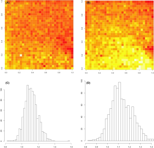
We first investigate the existence of spatial pattern. The HG-U95 chip has 640 × 640 spots on each array. We divided each array into sub-arrays of size 20 × 20. We run simple LTS regression on the target with respect to the reference for each sub-array. This results in an intercept matrix and a slope matrix of size 32 × 32, representing the spatial difference between target and reference in background and scale. We first take Array M as the common reference. The slope matrices of Array P and M are shown in Figure 1A and B, respectively, and their histograms are shown in Figure 1C and D. Two quite different patterns are observed. Similar phenomenon exists in patterns of α. The key observation is that spatial patterns are array-specific and unpredictable to a great extent. This justifies the need of adaptive normalization.

Figure 1.

The slope matrices of two arrays show different spatial patterns in scale. The common reference is Array M. (A) Array P versus M; (B) Array N versus M. (C and D) Their histograms are shown at bottom correspondingly.

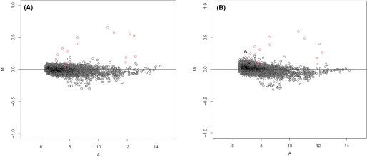
We carry out SUB-SUB normalization to each of the eight arrays using Array M as the reference. We experimented with different sub-array sizes, overlapping sizes and trimming fractions. Figure 2 shows the M–A plots summarized from the eight arrays after normalization, namely, the log-ratios of expressions between the two groups versus the abundance. The sub-array size is 20 × 20, the overlapping size is 10 and the trimming factor are 0.4 and 0 in the subplots Figure 2A and B, respectively. Our result indicates that both the sub-array size (data not shown) and trimming fraction matter substantially for normalization. In other words, stratification by spatial neighborhood and selection of breakdown value in LTS do contribute a great deal to normalization. Overlapping size has a little contribution in this dataset. Our method identifies 14 of the 16 differentially expressed spike-in gene with only a few false positives (Figure 2A).

Figure 2.

M–A plots of spike-in data after SUB-SUB normalization: (A) trimming fraction is 0.4; (B) trimming fraction is 0.

Perturbed spike-in dataset

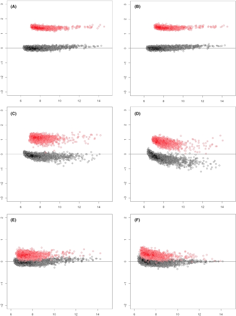
SUB-SUB normalization protects substantial differentiation by selecting an appropriate trimming fraction in LTS. To test this, we generate an artificial dataset with relatively large fraction of differentiation by perturbing the HG-U95 spike-in dataset. Namely, we randomly choose 20% genes and increase their corresponding probe intensities by 2.5-fold in the four arrays in the second group. We then run SUB-SUB normalization on the perturbed dataset with various trimming fractions. The results are shown in Figure 3A, B, C, D for four trimming fractions, 50, 30, 20 and 10%. The normalization is satisfactory when the trimming fraction is >30%, or 10% larger than the nominal differentiation fraction. The extra fraction may account for random variation. In another case, we randomly choose 20% genes and increase their corresponding probe intensities by 1.5-fold. The results corresponding to the trimming fraction 50 and 0% are shown in Figure 3E and F respectively. We note that the black dots are blocked by red ones in these two subplots when they overlap.

Figure 3.

(A–F)M–A plots of perturbed spike-in dataset after SUB-SUB normalization. The x-axis is the average of log-intensities from two arrays. The y-axis is their difference after normalization. In the top four subplots, 20% randomly selected genes have been artificially up-regulated by 2.5-fold in Array Q, R, S and T. The differentiated genes are marked red, and undifferentiated genes are marked black. The trimming fractions in the subplots are: A, 50%; B, 30%; C, 20%; D, 10%. In the two subplots at the bottom, 20% randomly selected genes have been artificially up-regulated by 1.5-fold in Array Q, R, S and T. The trimming fractions are: E, 50%; F, 0%.

Primate brain expression dataset

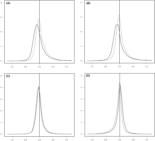
Compared with other primate brains, such as chimpanzee and orangutan, a relatively high percentage of genes are differentially expressed in human brains, and most of them are up-regulated in human brains (19,20). Moreover, the chimpanzee and orangutan samples are hybridized with human HG-U95 chips, so it is reasonable to assume if there were any measurement bias in primate mRNA expressions compared with humans, it would be a downward bias. Figure 4A–D shows the density functions of log-ratios of gene expressions for four cases: HUMAN 1 versus ORANG.; HUMAN 2 versus ORANG.; HUMAN 1 versus CHIMP. 1; HUMAN 1 versus HUMAN 2. The results from SUB-SUB (trimming fraction is 20%) and quantile normalization are plotted in red and blue, respectively. When comparing humans with primates, the distribution resulted from the SUB-SUB method is to the right of that resulted from the quantile method. This is more obvious in the cases of humans versus orangutan, which are more genetically distant from each other than other cases do; see Figure 4E and F. As expected, the distributions skew to the right and the long tails on the right might have a strong influence on the quantile normalization, which aims to match marginal distributions from humans and primates in a global fashion. However, in the cases of HUMAN 1 versus ORANG. and HUMAN 2 versus ORANG., the modes corresponding to the quantile method are in the negative territory while the modes corresponding to SUB-SUB method are closer to zero. The results from SUB-SUB normalization seem to be more reasonable. Furthermore, the difference in the case of HUMAN 1 versus HUMAN 2 is more distinct than that in the case of HUMAN 1 versus CHIMP. 1; see the two subplots at the bottom. The analysis in (17) also indicates that HUMAN 2 differs more from other human samples than the latter differ from the chimpanzee samples. We checked the M–A plot of HUMAN2 versus ORANG after SUB-SUB normalization (figure not shown) and observed that HUMAN 2 has more up-regulated genes than down-regulated genes compared with ORANG.

Figure 4.

The densities of expression log-ratios between: (A) HUMAN 1 versus ORANG.; (B) HUMAN 2 versus ORANG.; (C) HUMAN 1 versus CHIMP. 1; (D) HUMAN 1 versus HUMAN 2. The results from SUB-SUB normalization (trimming fraction is 20%) and quantile normalization are represented by dotted and solid line, respectively.

Variation reduction by sub-array normalization

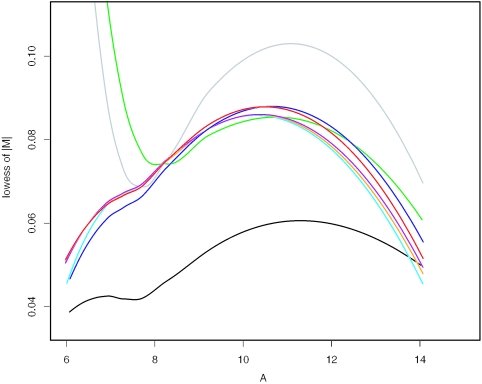
Stratification is a statistical technique to reduce variation. Sub-array normalization can be regarded as a way of stratification. We normalize the yeast array 2-121502 versus 2-121501 by various normalization methods available from Bioconductor. Since the two arrays are replicates, the difference between them is due to experimental variation. In the resulting M–A plots, we fit lowess (3) curves to the absolute values of M, or |M|. These curves measure the variation between the two arrays after normalization (see Figure 5). The sub-array normalization achieves the minimal variation. As variation is reduced, signal-to-noise ratio is enhanced and power of significance tests is increased.

Figure 5.

The lowess curves of |M| versus A values by various normalization methods. Gray: no normalization; black: sub-sub; red: quantiles; green: constant; purple: contrasts; blue: invariant-set; orange: lowess; cyan: qspline.

Other normalization procedures can be applied at the sub-array level as well. For example, if differentiation is not substantial, we can apply quantile, lowess, qspline normalization, etc. We note that different statistical methods, especially those non-parametric ones, may have specific requirements on the sample size. To achieve statistical effectiveness, we need to select the size of sub-array for each normalization method.

DISCUSSION

External controls

In cDNA arrays, some designs use external RNA controls to monitor global messenger RNA changes, (16). In our view, external RNA controls play the role of undifferentiated probe sets. To carry out local normalization, we need quite some number of external controls for each subgrid. In current Affymetrix arrays, this is not available.

Differentiation fraction

In many microarray experiments, our primary goal is the identification of differentially expressed genes. But the degree of differentiation may be quite different from one case to another. Next, we briefly mention some cases in which a large fraction of genes may be differentially expressed between two samples. First, in one study of the life span of yeast, we compare expression profiles of a wild-type strain with another, such as sch9Δ. The metabolism in the knock-out strain is greatly reduced and this leads to life span extension (21). Second, gene chips for some organisms are not available. Cross-species hybridization is a useful strategy for comparative functional genomics. The comparison of brain expressions of humans versus primates discussed earlier is one such example. Third, some customized arrays are so designed that only probes of hundreds of genes relating to a specific biological pathway are included for the consideration of cost. SUB-SUB normalization uses LTS to identify a ‘base’ subset of probes for adjusting difference in background and scale. In theory, the method can be applied to microarray experiments with differentiation fractions as high as 50%. In addition, our method does not assume an equal percentage of up- and down-regulated genes. In the mean time, LTS keeps the statistical efficiency advantage of least squares.

Nonlinear array transformation versus linear sub-array transformation

To eliminate the nonlinear phenomenon seen in M–A plots or Q–Q plots, methods such as lowess, qspline and quantile normalization use nonlinear transformation at the global level (6,7,22). In comparison, we apply a local strategy in SUB-SUB normalization. One array is split into sub-arrays and a simple linear transformation is fitted for each sub-array. With an appropriate sub-array size and trimming fraction, the nonlinear feature observed in M–A plots is effectively removed by linear sub-array transformation to a great extent. We speculate that the nonlinear phenomenon is partially caused by spatial variation. One simulation study also supports this hypothesis, but further investigation is required. Next, we give one remark regarding nonlinearity. In normalization, we adjust the intensities of a target array compared with those of a reference. Even though the dye effect is a nonlinear function of spot intensities, a linear transformation may be a good approximation as long as the majority of probe intensities from the target and reference are in the same range and thus have similar nonlinear effect. Occasionally when the amount of mRNA from two arrays is too different, slight nonlinear pattern is observed even after sub-array normalization. To fix the problem, we can apply global lowess after the sub-array normalization. Alternatively, to protect substantial differentiation, we can apply a global LTS normalization subject to a differentiation fraction once more.

Transformation

The variance stabilization technique was proposed in relation to normalization (23,24). We have tested SUB-SUB normalization on the log-scale of probe intensities, but the result is not as good as that obtained on the original scale. After normalization, a summarization procedure reports expression levels from probe intensities. we have tried the median polishing method (18) on the log-scale. Alternatively, we can do a similar job on the original scale using MBEI (25).

Usage of MM probes

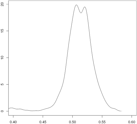
Some studies suggested using PM probes only in Affymetrix chips (26). We checked the contribution of MM probes and PM probes to the subsets associated with LTS regressions from all sub-arrays. Figure 6 shows the distribution of the percentage of MM probes in the subsets identified by LTS. Our result shows that MM probes contribute slightly more than PM probes in LTS regression, mostly in the range 46–56%.

Figure 6.

Histogram of percentages of MM probes in the subsets associated with LTS.

Diagnosis

The detection of bad arrays is a practical problem in the routine data analysis of microarrays. In comparison with the obvious physical damages, such as bubbles and scratches, subtle abnormalities in hybridization, washing and optical noise are more difficult to detect. By checking values of α and β in LTS across sub-arrays, we can detect bad areas in an array and save information from the rest areas. Consequently, we can report partial hybridization result instead of throwing away an entire array.

REFERENCES

- 1.Affymetrix Microarray Suite User Guide, 5th edn. Santa Clara, CA: Affymetrix; 2001. [Google Scholar]
- 2.Lockhart D.J., Dong H., Byrne M.C., Follettie M.T., Gallo M.V., Chee M.S., Mittmann M., Want C., Kobayashi M., Horton H., Brown E.L. DNA expression monitoring by hybridization of high density oligonucleotide arrays. Nat. Biotechnol. 1996;14:1675–1680. doi: 10.1038/nbt1296-1675. [DOI] [PubMed] [Google Scholar]
- 3.Cleveland W.S. Robust locally weighted regression and smoothing scatterplots. J. Am. Stat. Assoc. 1979;74:829–836. [Google Scholar]
- 4.Yang Y.H., Dudoit S., Luu P., Speed T.P. Normalization for cDNA microarray data. In: Bittner M.L., Chen Y., Dorsel A.N., Dougherty E.R., editors. Microarrays: Optical Technologies and Informatics. SPIE Vol. 4266. [Google Scholar]
- 5.Sidorov I.A., Hosack D.A., Gee D., Yang J., Cam M.C., Lempicki R.A., Dimitrov D.S. Oligonucleotide microarray data distribution and normalization. Inform. Sci. 2002;146:67–73. [Google Scholar]
- 6.Workman C., Jensen J., Jarmer H., Berka R., Gautier L., Nielsen B., Saxild H., Nielson C., Brunak S., Knudsen S. A new nonlinear normalization method for reducing variability in DNA microarray experiments. Genome Biol. 2002;3:1–16. doi: 10.1186/gb-2002-3-9-research0048. [DOI] [PMC free article] [PubMed] [Google Scholar]
- 7.Bolstad B., Irizarry R.A., Astrand M., Speed T.P. A comparison of normalization methods for high density oligonucleotide array data based on bias and variance. Bioinformatics. 2003;19:185–193. doi: 10.1093/bioinformatics/19.2.185. [DOI] [PubMed] [Google Scholar]
- 8.Zien A., Aigner T., Zimmer R., Lengauer T. Centralization: a new method for the normalization of gene expression data. Bioinformatics. 2001;17:323–331. doi: 10.1093/bioinformatics/17.suppl_1.s323. [DOI] [PubMed] [Google Scholar]
- 9.Li L.M. Blind inversion needs distribution (BIND): the general notion and case studies. In: Goldstein D., editor. Science and Statistics: A Festschrift for Terry Speed. Vol. 40. Bethesda, MD, USA: Institute of Mathematical Statistics; 2003. pp. 273–293. [Google Scholar]
- 10.Schadt E.E., Li C., Su C., Wong W.H. Analyzing high-density oligonucleotide gene expression array data. J. Cell. Biochem. 2000;80:192–202. [PubMed] [Google Scholar]
- 11.Schadt E.E., Li C., Ellis B., Wong W.H. Feature extraction and normalization algorithms for high-density oligonucleotide gene expression array data. J. Cell. Biochem. Suppl. 2001;37:120–125. doi: 10.1002/jcb.10073. [DOI] [PubMed] [Google Scholar]
- 12.Tseng G.C., Oh M., Rohlin L., Liao J.C., Wong W.H. Issues in cDNA microarray analysis: quality filtering, channel normalization, models of variations and assessment of gene effects. Nucleic Acids Res. 2001;29:2549–2557. doi: 10.1093/nar/29.12.2549. [DOI] [PMC free article] [PubMed] [Google Scholar]
- 13.Kepler T., Crosby L., Morgan K. Normalization and analysis of DNA microarray data by self-consistensy and local regression. Genome Biol. 2002;3:1–12. doi: 10.1186/gb-2002-3-7-research0037. [DOI] [PMC free article] [PubMed] [Google Scholar]
- 14.Rousseeuw P.J., Leroy A.M. Robust Regression and Outlier Detection. New York: Wiley; 1987. [Google Scholar]
- 15.Li L.M. An algorithm for computing exact least trimmed squares estimate of simple linear regression with constraints. Comput. Stat. Data Anal. 2004;48:717–734. [Google Scholar]
- 16.van de Peppel J., Kemmeren P., van Bakel H., Radonjic M., van Leenen D., Holstege F.C.P. Monitoring global messenger RNA changes in externally controlled microarray experiments. EMBO Rep. 2003;4:387–393. doi: 10.1038/sj.embor.embor798. [DOI] [PMC free article] [PubMed] [Google Scholar]
- 17.Enard W., Khaitovich P., Klose J., Zöllner S., Heissig F., Giavalisco P., Nieselt S., Muchmore E., Varki A., Ravid R., et al. Intra- and interspecific varaiation in primate gene expression patterns. Science. 2002;296:340–343. doi: 10.1126/science.1068996. [DOI] [PubMed] [Google Scholar]
- 18.Irizarry R.A., Hobbs B., Collin F., Beazer-Barclay Y.D., Antonellis K.J., Scherf U., Speed T.P. Exploration, normalization, and summaries of high density oligonucleotide array probe level data. Biostatistics. 2003;4:249–264. doi: 10.1093/biostatistics/4.2.249. [DOI] [PubMed] [Google Scholar]
- 19.Caceres M., Lachuer J., Zapala A., Redmond C., Kudo L., Geschwind H., Lockhart J., Preuss M., Barlow C. Elevated gene expression levels distinguish human from non-human primate brains. Proc. Natl Acad. Sci. USA. 2003;100:13030–13035. doi: 10.1073/pnas.2135499100. [DOI] [PMC free article] [PubMed] [Google Scholar]
- 20.Gu J., Gu X. Induced gene expression in human brain after the split from chimpanzee. Trends Genet. 2003;19:63–65. doi: 10.1016/s0168-9525(02)00040-9. [DOI] [PubMed] [Google Scholar]
- 21.Fabrizio P., Pozza F., Pletcher S.D., Gendron C., Longo V.D. Regulation of longevity and stress resistance by sch9 in yeast. Science. 2001;292:288–290. doi: 10.1126/science.1059497. [DOI] [PubMed] [Google Scholar]
- 22.Yang Y.H., Dudoit S., Luu P., Lin D.M., Peng V., Ngai J., Speed T.P. Normalization for cDNA microarray data: a robust composite method addressing single and multiple slide systematic variation. Nucleic Acids Res. 2002;30:e15. doi: 10.1093/nar/30.4.e15. [DOI] [PMC free article] [PubMed] [Google Scholar]
- 23.Durbin B.P., Hardin J.S., Hawkins D.M., Rocke D.M. A variance-stabilizing transformation for gene-expression microarray data. Bioinformatics. 2002;18:S105–S110. doi: 10.1093/bioinformatics/18.suppl_1.s105. [DOI] [PubMed] [Google Scholar]
- 24.Huber W., Heydebreck V., Sültmann H., Poustka A., Vingron M. Variance stabilization applied to microarray data calibration and to the quantification of differential expression. Bioinformatics. 2002;18:S96–S104. doi: 10.1093/bioinformatics/18.suppl_1.s96. [DOI] [PubMed] [Google Scholar]
- 25.Li C., Wong W.H. Model-based analysis of oligonucleotide arrays: model validation, design issues and standard error applications. Genome Biol. 2001;2:1–11. doi: 10.1186/gb-2001-2-8-research0032. [DOI] [PMC free article] [PubMed] [Google Scholar]
- 26.Wu Z., Irizarry R.A. San Diego, CA: 2004. Stochastic models inspired by hybridization theory for short oligonucleotide arrays; pp. 98–106. RECOMB 2004. [DOI] [PubMed] [Google Scholar]