On The Classic And Modern Theories Of Matching

Abstract

Classic matching theory, which is based on Herrnstein's (1961) original matching equation and includes the well-known quantitative law of effect, is almost certainly false. The theory is logically inconsistent with known experimental findings, and experiments have shown that its central constant-k assumption is not tenable. Modern matching theory, which is based on the power function version of the original matching equation, remains tenable, although it has not been discussed or studied extensively. The modern theory is logically consistent with known experimental findings, it predicts the fact and details of the violation of the classic theory's constant-k assumption, and it accurately describes at least some data that are inconsistent with the classic theory.

Thirty-five years ago, Richard J. Herrnstein (Herrnstein, 1970) proposed the theory of matching, according to which all behavior can be conceptualized as choice, governed by the matching equation

In this equation the Rs represent response rates or counts, the rs represent reinforcement rates or counts, and the numerical subscripts refer to the two components of a concurrent schedule (Herrnstein, 1961). The equation asserts that organisms allocate their behavior across concurrently available response alternatives in the same proportion that reinforcements are allocated across those alternatives.

Herrnstein (1970) turned the purely descriptive matching equation into a theory by applying it to single-alternative schedules. He conceptualized these as two-component concurrent schedules consisting of instrumental responding as one alternative, and background or extraneous responding as the other alternative. For this conceptualization of the single-alternative case, the matching equation can be written

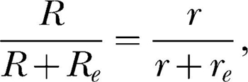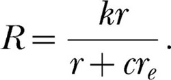
where R and r refer to the instrumental response and reinforcement rates or counts, and R_e and r_e refer to the extraneous response and reinforcement rates or counts. Assuming a constant total amount of behavior to allocate, k, then R + R_e  =  k, and the equation can be written

This is the well-known quantitative law of effect (de Villiers, 1977; de Villiers & Herrnstein, 1976), which has been widely and very successfully applied to single-alternative responding (McDowell, 1988). It follows from Equation 2 that responding in each component of a concurrent schedule must be described by

and

where the constant total amount of behavior, k, is allocated among three response alternatives, including the extraneous alternative. This brings the theory full circle inasmuch as Equations 3 and 4 can be combined to yield Equation 1, thereby establishing the theory's consistent account of single- and multiple-alternative environments.

Equation 1 to 4 constitute the fundamental statement of matching theory in its classic, or strict, formulation. The equations are listed in the left panels of Figure 1 for reference. A great deal of research since 1970 has shown that Equation 1 does not describe concurrent schedule data very well (Baum, 1974), but that, oddly, Equation 2 describes single schedule data quite well (McDowell, 1988). Equations 3 and 4 have not been studied extensively. As will be discussed in more detail later, the general success of Equation 2 is illogical, given the limited success of the equation from which it was derived (Equation 1).

Fig. 1. The equations of classic (left panels) and modern (right panels) matching theory.

The equations are referred to in the text by the numbers that appear in the upper left corner of each panel. The modern equations entail bias parameters and exponents, whereas the classic equations do not. The equations in the first row are the foundational equations of each theory, from which the remaining equations are derived. The modern equations reduce to the classic equations when all bias parameters and exponents equal unity (Equations 5 and 9 both reduce to the ratio form of Equation 1, that is, R₁/R₂  =  r₁/r₂).

The shortcomings of Equation 1 (e.g., Myers & Myers, 1977) quickly gave rise to a new form of descriptive matching in concurrent schedules (Baum, 1974; Staddon, 1968, 1972), namely, the now-familiar power function,

that has been very successful in describing behavior on concurrent schedules. Just as Equation 1 was the starting point of classic matching theory, Equation 5 is the starting point of what might be referred to as modern, or generalized, matching theory. The purpose of this paper is to examine the modern theory of matching, which has neither been discussed nor studied extensively, and to compare it with the classic theory.

THE MODERN THEORY

The modern theory of matching is obtained in the same way that Herrnstein obtained the classic theory, except that the point of departure is Equation 5 rather than Equation 1. The details of the calculations have been presented elsewhere (McDowell, 1986). The first result is a single-alternative equation analogous to Equation 2,

Just as in classic matching theory, this equation is obtained by assuming that a constant amount of behavior, k, is allocated among the available response alternatives, which in the single-alternative case are the instrumental alternative and the aggregate extraneous alternative. Notice that the total amount of behavior, k, and reinforcement for responding on the extraneous alternative, r_e, appear in this equation just as they appear in Equation 2. New to Equation 6 is the exponent, a, and the bias parameter, b, which are inherited, so to speak, from Equation 5 (McDowell, 1986).

Just as single-alternative forms for each component of a concurrent schedule were obtained from Equation 2 in the classic theory, analogous single-alternative forms for each component of a concurrent schedule can be obtained from Equation 6 in the modern theory (McDowell, 1986). These are

and

Each equation expresses response rate in one component of a concurrent schedule as a joint function of the reinforcement rates in both components (r₁ and r₂), just as do the analogous classic Equations 3 and 4. Notice also that k and r_e appear in Equations 7 and 8 just as they do in Equations 3 and 4. New to Equations 7 and 8 are three bias parameters, b₁₂, b_1e, b_2e, and three exponents, a₁₂, a_1e, a_2e. One bias parameter and one exponent apply to each of the three possible pairs of reinforcement rates that are compared as ratios in Equation 7 and 8. The subscripts refer to the response alternatives; 1 and 2 refer to the two components of the concurrent schedule and e refers to the extraneous alternative. Reinforcement rates from the two components of the concurrent schedule, r₁ and r₂, are compared as a ratio in the second term inside the square brackets of both Equation 7 and 8. Notice that the second term inside the square brackets of 8 is the reciprocal of the second term inside the square brackets of Equation 7, and that this term also constitutes the right side of Equation 5 (although the subscripts on the bias parameter and exponent are omitted from Equation 5). Reinforcement rates from the first component of the concurrent schedule and from the extraneous alternative, r₁ and r_e, are compared as a ratio in the first term inside the square brackets of Equation 7. Reinforcement rates from the second component of the concurrent schedule and from the extraneous alternative, r₂ and r_e, are compared as a ratio in the first term inside the square brackets of Equation 8. Each of these ratios is modified by the appropriate bias parameter and exponent.

It is important to recognize that the forms of Equations 6 to 8 are not arbitrary. Their structure is a formal consequence of applying the logic of Herrnstein's matching theory to Equation 5 (McDowell, 1986). Just as Equations 3 and 4 can be combined to obtain Equation 1, the quotient of Equation 7 and 8 produces Equation 5, which brings the modern theory full circle, and demonstrates the consistency of the modern theory's single- and multiple-alternative accounts.

Equations 5 to 8 of the modern theory are analogous to Equation 1 to 4 of the classic theory. Equation 1 and Equations 5 are the foundational descriptive equations for each version of the theory. The remaining equations are derived from the foundational equation via the same logic for both classic and modern theories. McDowell (1986) showed that the modern theory entails a fifth equation, which applies to concurrent schedules. This equation,

is similar to Equations 5, but includes the other two bias parameters and the other two exponents from the set of parameters entailed by the modern theory. McDowell (1986) showed that Equations 9 is a consequence of matching theory's requirement that all behavior be allocated among the available response alternatives, with none left over. Notice that the right side of Equations 9 is the product of two reinforcement rate ratios, each raised to the appropriate exponent and multiplied by the appropriate bias parameter. The first ratio in the equation compares the reinforcement rates from the second component of the concurrent schedule and from the extraneous alternative, r₂ and r_e. This ratio, together with its exponent and bias parameter, is identical to the first term inside the square brackets in Equations 8. The second ratio compares the reinforcement rates from the first component of the concurrent schedule and from the extraneous alternative, r₁ and r_e. This ratio, together with its exponent and bias parameter, is identical to the reciprocal of the first term inside the square brackets in Equations 7. Although Equations 5, 7, 8, and Equations 9 are notationally complicated, their structure is simple. They consist entirely of unity, the parameter k, and the following three quantities and their reciprocals:

The five equations of modern matching theory are listed in the right panels of Figure 1 for reference.

The equations of classic matching theory are special cases of the equations of modern matching theory. The latter reduce to the former when all bias parameters and exponents equal unity. Specifically, Equations 5 and 9 both reduce to the ratio form of Equations 1, Equations 6 reduces to Equations 2, and Equations 7 and 8 reduce to Equations 3 and 4.

THE LOGIC OF MATCHING THEORY

Thirty-five years of research on matching theory have made at least three things clear (,McDowell, 1988, 1989): Equation 5, the foundational equation of the modern theory, accounts for concurrent-schedule data very well; Equations 1, the foundational equation of the classic theory does not; and Equation 2, the single-alternative equation of the classic theory accounts for single-schedule data very well.

Given this empirical information, the first test of matching theory must be logical. Consider the classic theory. Because the foundational equation upon which this theory is built is not generally consistent with data, it seems unlikely that the theory (Equations 2 to 4) is correct. The classic theory does not allow for asymmetries in choice (i.e., a bias parameter not equal to 1), or for undercontrol or overcontrol of response allocation by reinforcer distribution (i.e., an exponent on the ratio of reinforcement rates not equal to 1). These are the reasons the foundational equation of the theory (Equation 1) has limited applicability; it makes sense to suppose that these reasons limit the remainder of the equations as well. For example, how likely is it that a food-deprived animal shows no bias for food reinforcement over extraneous background reinforcement on a single schedule? Similarly, we know that the exponent on power function matching (Equation 5) is typically about 0.8 for behavior on concurrent schedules (Baum, 1974), indicating a degree of undercontrol of response allocation by reinforcer distribution. Why should the same not be true in single schedules? The modern theory of matching permits asymmetries in choice, and undercontrol or overcontrol of response allocation by reinforcer distribution. Moreover, the foundational equation of this theory (Equation 5) is known to provide an excellent description of behavior on concurrent schedules. This does not mean, of course, that the modern theory is necessarily correct; it only means that the theory is not logically inconsistent with experimental findings and is therefore logically tenable.

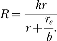
This logical analysis is marred by the curious fact that Equation 2, the classic theory's single-alternative equation, is quite successful in describing data (McDowell, 1988). But how can it be that there is no bias on single schedules, and that there is perfect control of response allocation by reinforcer distribution? Let us look first at bias.Equation 2, and Equation 6 with the exponent, a, set equal to 1 are

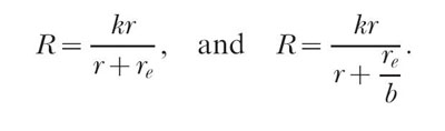Fitting Equation 2 entails estimating k and r_e. Fitting the above version of Equation 6 entails estimating k and r_e/b. Notice that r_e and b cannot be estimated independently; only their ratio can be estimated. Suppose for a moment that Equation 6 is true and that an experimenter fits it to a set of data, obtaining values for k and r_e/b. Now suppose the experimenter increases the bias for the instrumental alternative by increasing the magnitude of the reinforcer, and then obtains a second set of data using the larger magnitude, and a second set of estimates of k and r_e/b. Because the bias parameter has increased, the estimated value of r_e/b will be smaller for the second set of data. A classic theorist who fits Equation 2 to these data will find that r_e has decreased, and will explain this by saying that the units on r_e have changed, that is, r_e is now being measured in the larger units of the new instrumental reinforcer and so the same background level of reinforcement is described by a smaller number. Ignoring for the time being the merits of the classic theorist's point of view, this example shows that the hyperbolic form of Equation 2 will provide an excellent description of single schedule data in the presence of bias that is consistent with the modern theory. In fact, the description provided by Equation 2 (specifically, the percentage of variance accounted for) will be identical to the description provided by the version of Equation 6 given above. According to the modern theory, when bias changes, the value of the parameter in the denominator of either equation will change in the opposite direction. The form of the equation is not affected, and hence the two equations will provide identical fits.

Unlike the bias parameter, the exponent in Equation 6 does change the form of the function, but not by much. Consider Equation 7 without bias (i.e., b  =  1):

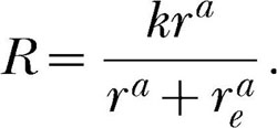Simulated data calculated from this equation with k  =  100, r_e  =  50 and a  =  0.65 are plotted as filled circles in the top left panel of Figure 2. The smooth curve is the best fit of the classic single-alternative form, Equation 2. The proportion of variance accounted for by this equation is 0.98, clearly what would be referred to as a good fit. But, as is evident from the figure, the residuals left by the fit are not random; the data overshoot the curve at low and high reinforcement rates and undershoot it at intermediate reinforcement rates. The plot of the standardized residuals against the predicted response rates in the upper right panel of Figure 2 reveals this systematic pattern in the residuals. It can be shown that the closer the exponent is to unity, the smaller the deviations from the classic Equation 2. Consider an exponent of 0.8, which is about what one would expect on the basis of concurrent schedule research. Simulated data calculated using this exponent, and the same k and r_e as before, with random homoscedastic gaussian error added to the response rates (standard deviation  =  four responses per minute), produces the data points that are plotted as filled circles in the bottom left panel of Figure 2. Again, the smooth curve is the best fit of the classic single-alternative form, Equation 2, which accounts for 97% of the variance of these simulated response rates. Again, this appears to be a good fit. But now, in the presence of error in the response rates, it is difficult to detect a pattern in the residuals. This is because the random error in the response rates masks the small systematic deviations from Equation 2. The plot of the standardized residuals against the predicted response rate in the lower right panel of the figure also fails to show a clear pattern. Additional details about these simulations can be found in the Appendix.

Fig. 2. The filled circles in the left panels are simulated response rates calculated from Equation 6 with k  =  100, r_e  =  50 and a  =  0.65 (top) or 0.80 (bottom).

In the top left panel the response rates are errorless; in the bottom left panel the response rates include random homoscedastic gaussian error with a standard deviation of four responses per minute. The smooth curve in each panel is the best fit of Equation 2; the proportion of variance accounted for (pVAF) by the fit is given in the lower right of each panel. The right panels show the standardized residuals for each fit plotted against the predicted response rates.

It is now evident why Equation 2 describes single schedule data well, even though it may not be the correct account. Bias will not affect the quality of the fit of Equation 2; it will only affect the size of r_e. A value of the exponent, a, that is close to but different from unity will introduce a small but systematic deviation from the fit of Equation 2. But because this deviation is small, Equation 2 still will account for a large proportion of the response rate variance. In addition, the error in measuring response rates may swamp the systematic deviation, thus making it difficult or impossible to detect in the residuals.

These simulations support the logical analysis of the classic and modern theories of matching presented here. Despite the empirical success of Equation 2, the classic theory, because its foundational equation is known to have limited applicability, is not itself likely to be widely applicable.

TESTING MATCHING THEORY USING SINGLE SCHEDULES

Needless to say, logic alone is not sufficient reason to discard a theory. Empirical tests of the theory have focused on its fundamental assumption, namely, that a constant amount of behavior, k, is allocated among available response alternatives (Herrnstein, 1974). Early reviews (de Villiers, 1977; McDowell, 1980; Warren-Boulton, Silberberg, Gray, & Ollom, 1985; Williams, 1988) reported mixed findings, with some experimenters reporting the required constant k, and others reporting a k that varied with reinforcement parameters such as magnitude. In a recent review, Dallery, McDowell, and Soto (2004) reached the following conclusion:

Recent research suggests that k remains constant over a limited range of reinforcer magnitudes (Dallery, McDowell, & Lancaster, 2000; McDowell & Dallery, 1999), and these results are consistent with two prior studies (Heyman & Monaghan, 1987, 1994). However, if the range of magnitudes is extended, then k varies markedly (Dallery et al., 2000; McDowell & Dallery, 1999). (p. 46)

The literature reviewed by Dallery et al. (2004) shows that k varies directly with reinforcer magnitude, and that the variation is small at large magnitudes but becomes larger at small magnitudes. This helps explain the mixed outcomes in the literature and supports the conclusion that the central assumption of the classic theory is false.

The violation of the constant-k requirement of the classic theory is predicted by at least one other theory, namely, linear system theory (McDowell, 1980; McDowell, Bass, & Kessel, 1993; McDowell & Kessel, 1979). Interestingly, it also is predicted by the modern theory of matching. This can be shown by conducting a simulated experiment analogous to experiments that have been conducted to test the constant-k requirement of the classic theory. For this simulated experiment, the modern theory of matching will be assumed to be correct. According to the modern theory, varying reinforcer magnitude corresponds to varying the bias parameter in Equation 6. Larger reinforcer magnitudes generate a larger bias in favor of the instrumental reinforcer; smaller magnitudes generate a smaller bias, and very small magnitudes may even produce bias that favors the background reinforcement. In the simulated experiment, reinforcer magnitude was varied by varying the bias parameter in Equation 6. Fifteen sets of simulated data were calculated from Equation 6 with k  =  100, a  =  0.8, r_e  =  5, 25, or 100, and with a bias parameter of 0.1, 0.4, 1, 1.2, or 1.5. For each set of simulated data, 16 reinforcement rates that ranged from 5 to 400 were used to calculate response rates; error was not added to these rates. The classic single-alternative Equation 2 was fitted to each set of data, which yielded 15 estimates of k. These estimates are plotted in Figure 3 as a function of the bias parameter used to generate the data from which the estimate was obtained.

Fig. 3. Values of k estimated by fitting Equation 2 to data generated by Equation 6 with parameters set equal to the values given in the figure. Changes in the bias parameter along the x-axis correspond to changes in the magnitude of the instrumental reinforcer.

For the top curve in Figure 3, r_e in Equation 6 was set equal to 5. This might correspond to a typical experiment in an operant chamber, where the background reinforcement is relatively infrequent. At this value of r_e, the k estimated from Equation 2 remained nearly constant across a large range of bias parameters, and hence simulated reinforcer magnitudes, but declined at the very low end of the range. The other two curves in the figure show the same pattern, except that the decline in k was more marked the larger the value of r_e. Evidently, the direct variation of the classically estimated k with bias that is shown in Figure 3 is consistent with the experimental findings reviewed by Dallery et al. (2004). These findings, it is now clear, are consistent with the modern theory of matching.

If modern matching theory predicts a classic k that varies with reinforcer magnitude, then this theory, which itself entails a constant k, should accurately describe a set of data that shows this variation. Consider an experiment by McDowell and Dallery (1999) in which 5 rats were deprived of water for varying amounts of time and then worked on variable interval (VI) schedules of water reinforcement. The duration of water deprivation was considered to affect the reinforcing value of a 0.025-ml water reinforcer, and hence different durations of water deprivation were considered analogous to different reinforcer magnitudes. McDowell and Dallery found that the k estimated from the classic Equation 2 decreased with decreasing water deprivation for all 5 rats, thus violating the constant-k requirement of the classic theory.

One way to evaluate the modern theory's description of these data is to fit Equation 6,

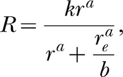simultaneously to the data from all deprivation conditions for each rat using a single, shared, k and a single, shared, a. The single k parameter is required by the modern theory, inasmuch as k is required to remain constant across changes in reinforcer properties. Using a single a parameter for all deprivation conditions is not specifically required by the theory but arguably constitutes the most conservative application of the theory to data. The third parameter entailed by Equation 6 is r_e^a/b, which, as mentioned earlier, must be estimated as a unit. This parameter must be allowed to vary across deprivation conditions because different levels of deprivation are likely to produce different degrees of bias, b, for the water reinforcer. For a given set of parameter values (i.e., a single k, a single a, and as many values of r_e^a/b as there are deprivation conditions), Equation 6 will produce a residual sum of squares (RSS) for each deprivation condition. There also will be a constant total sum of squares (SS) for each deprivation condition. The ratio of these two quantities, RSS/SS, summed over the deprivation conditions, can be minimized by adjusting the set of parameters to obtain simultaneous, or ensemble, fits of Equation 6 to each rat's data. In other words, given four deprivation conditions, a single k, a single a and four r_e^a/bs can be found such that

where the numerical subscripts refer to each deprivation condition, is a minimum. Additional details about this fitting method are given in the Appendix. If (a) the ensemble fits of the theory are good, that is, if they account for a large proportion of the data variance, and if (b) the residuals left by the fits are random, and if (c) the parameter estimates obtained from the fits are reasonable and consistent with the theory, then the modern theory of matching may be said to provide a good description of the data.

This simultaneous, or ensemble, fitting method was applied to McDowell and Dallery's (1999) Phase 2 data (including the ∼24-hr deprivation condition). The results of the fits are listed in Table 1. All parameter estimates and percentages of variance accounted for (%VAF) are based on the rounded response and reinforcement rates reported in McDowell and Dallery's Appendix B. Quantities listed in Table 1 that also are reported in their article may differ because the latter were based on unrounded data.

Table 1. Estimated k and percentage of variance accounted for (%VAF) by individual fits of the classic Equation 2, and estimated k, a, and r_e^a/b, and %VAF for ensemble fits of the modern Equation 6 to data from McDowell and Dallery (1999).

Rat	Hour deprivation	Classic individual fits (Equation 2)		Modern ensemble fits (Equation 6)
		k	%VAF	k	a	{{r_e ^a } \over b}	%VAF
R1	23.5	80	96	81	0.94	77	96
	18	62	97			461	96
	12	87	100			443	100
	6	52	100			679	99
	4	30	95			1,025	95
	Overall		97				97
R2	23.5	97	99	116	0.85	131	100
	18	82	100			467	99
	12	48	100			605	99
	6	47	99			824	100
	Overall		99				100
R14	23.5	17	93	18	0.75	13	89
	18	16	99			60	98
	12	13	97			61	97
	6	4	84			180	83
	Overall		96				95
R16	23.5	115	99	178	0.86	751	99
	18	72	100			1,459	100
	12	16	100			2,478	99
	6	4	100			4,818	100
	Overall		99				99
R19	23.5	86	97	112	0.80	135	96
	18	69	99			408	98
	12	14	85			770	80
	6	11	99			1,382	99
	Overall		97				96

Consider first the individual fits of the classic Equation 2, which also are listed in Table 1. Equation 2 accounted for a large percentage of variance in virtually every condition, but the estimates of k declined from the longest to the shortest deprivation condition for all rats, which violates the classic theory of matching. Also listed in the table are overall %VAFs for each rat's Equation 2 fits. These were obtained using

for the n deprivation conditions to calculate the overall error variance associated with the fits considered as a group. Additional details about this method of calculating overall %VAFs are given in the Appendix.

The results of ensemble fits of the modern Equation 6 are given on the right side of Table 1. A single shared k and a single shared a are listed for each rat, along with estimates of r_e^a/b for each deprivation condition. As shown in the table, the %VAFs for the fits of Equation 6 were excellent, and not appreciably different from the %VAFs for the fits of the classic Equation 2. Notice that even though Equation 2 entails fewer parameters than Equation 6, the fits of Equation 2 required more free parameters per rat than did the fits of Equation 6. For example, with four deprivation conditions, the fits of Equation 2 required two parameters per condition, or eight free parameters per rat, whereas the ensemble fits of Equation 6 entailed one k, one a and four r_e^a/bs, or six free parameters per rat. The standardized residuals for the ensemble fits of Equation 6, pooled across deprivation conditions and rats, are plotted against the predicted response rates in Figure 4. As is evident from the figure, there were no clear trends in the residuals.

Fig. 4. Standardized residuals left by ensemble fits of Equation 6 to data from McDowell and Dallery (1999), pooled across deprivation conditions and rats, and plotted as a function of predicted response rates.

The estimates of a in Table 1 ranged from 0.75 to 0.94, which is consistent with values typically reported for concurrent schedules. According to the modern theory, the quantity r_e^a/b should increase as deprivation level decreases. This is because lesser degrees of deprivation are likely to generate lesser degrees of bias (b) favoring the water reinforcer. As b decreases with decreasing deprivation, r_e^a/b must increase. As shown in Table 1, the estimates of r_e^a/b for all rats showed this trend.

Clearly, all three criteria listed earlier were met by the fits of Equation 6 to these data. They accounted for a large proportion of the data variance and left random residuals, and the parameter estimates were reasonable and consistent with the theory. Although these data violate the constant-k requirement of classic matching theory, they are consistent with the constant-k requirement of the modern theory.

To summarize, it is illogical to expect that the classic theory of matching is correct, given known empirical results on concurrent schedules. Furthermore, outcomes of direct empirical tests of the theory indicate that its central assumption is false. In contrast, the modern theory of matching is logically consistent with known empirical results on concurrent schedules. In addition, it predicts the violation of the classic theory's central assumption, and it accounts for at least one set of data that exhibits this violation while maintaining inviolate its own constant-k requirement.

TESTING MATCHING THEORY USING CONCURRENT SCHEDULES

It is not widely recognized that every concurrent schedule constitutes a test of matching theory. An adequate test of the theory must engage the constant-k assumption that fuels the theory's derivation. The most obvious way to do this is by applying Equations 2 and 6 to behavior on single-alternative schedules. But every concurrent schedule also entails single-alternative equations that engage the constant-k assumption; these are Equations 3 and 4 in the classic theory and Equations 7 and 8 in the modern theory. The classic theory can be tested on a concurrent schedule by simultaneously fitting Equations 1 3, and 4 to the data; the modern theory can be tested by simultaneously fitting Equations 5, 7, 8, and 9 to the data. These fits must be evaluated with reference to the three criteria listed earlier, namely, quality of fit, randomness of residuals, and reasonableness and theoretical consistency of parameter estimates.

This ensemble method of testing matching theory will be illustrated with data from Dallery et al.'s (2004) study of rats working on concurrent VI VI and single VI schedules for sucrose pellets of differing concentrations. Data will be examined from 4 rats working on concurrent VI VI schedules where a 75% sucrose pellet was used as the reinforcer in one component and a 50% sucrose pellet was used as the reinforcer in the other component. To evaluate the classic theory, Equations 1, 3, and 4 were fitted simultaneously to each rat's data with a single k and a single r_e shared across the two components of the concurrent schedule. Although Equation 1 does not participate in the parameter estimation, it is included in the analysis so that its residuals can be examined. For each rat, a single k and a single r_e were found such that RSS₁/SS₁ + RSS₂/SS₂ was a minimum, where the first ratio in the sum refers to the first component of the concurrent schedule and to Equation 3, and the second ratio refers to the second component and to Equation 4. Percentages of variance accounted for (%VAF) by the ensemble fits are listed in the left columns of Table 2. The %VAFs for Equation 1 were obtained by calculating the residuals from the straight line described by the log transform of the ratio form of this equation.

Table 2. Percentage of variance accounted for by ensemble fits of classic theory Equations 1, 3, and 4 and modern theory Equations 9″, 7″, and 8″ to concurrent schedule data from Dallery, McDowell, & Soto (2004).

Rat	Classic equation number			Modern equation number
	1	3	4	9″	7″	8″
125	17	58	55	98	73	81
126	63	90	84	97	99	92
127	93	96	94	99	96	98
128	85	95	90	97	96	94
Median	74	93	87	98	96	93

As shown in the table, the equations of classic matching theory in some cases described the rats' behavior poorly and in other cases described it moderately well, although no %VAF exceeded 96%. By and large the worst fits were for Equation 1. The overall median %VAF for the three equations and 4 rats was 87.5%. If Rat 125's results are considered aberrant, then these fits could be judged to be at least satisfactory. But the residuals left by the fits were not random. The standardized residuals are plotted against the relevant predicted dependent variable in the left panels of Figure 5, pooled across rats. The straight lines are least squares fits to the plotted data. In the top left panel, the standardized residuals also are pooled across concurrent schedule components. The residuals in this panel were left by Equations 3 and 4, and show a decreasing trend across predicted response rates. The correlation coefficient for this plot was −0.35. Analogous correlation coefficients for individual rats in numerical order were −0.67, −0.78, −0.37, and −0.34, indicating that the declining trend was consistent across rats. The residuals in the bottom left panel of Figure 5 were left by the log transform of the ratio form of Equation 1; they also show a declining linear trend and a large negative correlation. Analogous correlation coefficients for individual rats in numerical order were −0.99, −0.96, −0.96, and −0.88, indicating that this trend also was consistent across rats.

Fig. 5. Standardized residuals left by ensemble fits of classic equations (left panels) and modern equations (right panels) to concurrent schedule data from Dallery, McDowell, & Soto (2004). Data are pooled across rats in all panels and also are pooled across concurrent schedule components in the top panels. The straight lines in all panels are least squares fits. Correlation coefficients are given in the upper right of each panel.

Although the %VAFs for the classic equations in Table 1 could be considered satisfactory, the residuals left by the fits were not random. It must be concluded, therefore, that these concurrent schedule data are not consistent with the classic theory of matching. Turning now to the modern theory, it is necessary to fit Equations 5, 7, 8, and 9 as an ensemble to each rat's data. The first step in fitting these equations is to recognize that not all the parameters in the equation can be estimated independently. Just as r_e^a/b in Equation 6 is a composite parameter that must be estimated as a unit, so too

in Equations 7, 8, and 9 are composite parameters that must be estimated as units. Letting c_1e represent the first of these composite parameters,

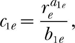and c_2e represent the second,

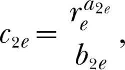we can write Equations 7, 8, and 9 as

and

which reduces the number of parameters in Equations 5, 7, 8, and 9 by one.

Any fit of the modern theory to concurrent schedule data must begin with Equations 5, 7′, 8′, and 9′, which entail a total of seven free parameters. A further simplification is possible, however, and probably desirable, and that is to set all three exponents to a single value. Unlike the bias parameters, it is not clear what variables, if any, affect the exponents in these equations. Therefore, a conservative approach is to set them equal to a single value, a, rather than allowing them to vary separately. A further benefit of this approach is that when the three exponents are equal, the three bias parameters and two composite parameters are related as

,

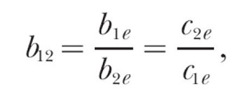and Equations 5 and 9 become identical. Hence, when all the exponents are equal, the four concurrent-schedule equations of modern matching theory entailing seven estimable parameters reduce to three equations entailing four estimable parameters. The three equations are

for responding in the first component of the concurrent schedule,

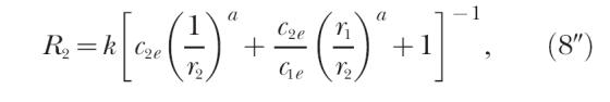for responding in the second component of the concurrent schedule, and

for the ratio of responding in the two components of the concurrent schedule. For all three equations, the exponents in c_1e and c_2e equal a. Equation 9″ could just as well be labeled Equation 5″, because the two equations are identical.

Equations 7″, 8″, and 9″ were fitted to the data discussed earlier from Dallery et al. (2004). The equations were fitted to each rat's data as an ensemble with single shared k, a, c_1e, and c_2e parameters. In other words, a single shared k, a, c_1e, and c_2e were found such that RSS₁/SS₁ + RSS₂/SS₂ + RSS₃/SS₃ was a minimum, where the first term in this sum refers to the first component of the concurrent schedule and to Equation 7″, the second term refers to the second component of the schedule and to Equation 8″, and the third term refers to the log ratios of responses and reinforcers and to Equation 9″. The %VAFs for these fits are listed in the right columns of Table 2. With a few exceptions, the fits were excellent, accounting for as much as 99% of the data variance. The fits of Equation 9″ were far superior to those of Equation 1, as might be expected, and the fits of Equation 7″ and 8″ exceeded those of Equation 7″ and Equations 3 and 4 in all but one case, in which they were equal. The standardized residuals left by the fits of Equation 7″ and 8″, pooled across rats and concurrent schedule components, are plotted against predicted response rates in the top right panel of Figure 5. The straight line in the panel is a least squares fit to the plotted data. Clearly there was no trend in these residuals. Correlation coefficients for individual rats' standardized residuals, in numeric order, and pooled across concurrent-schedule components, were −0.06, −0.04, −0.04, and 0.06, confirming the absence of trend for individual rats. The standardized residuals left by the fits of Equation 9″, pooled across rats, are plotted against predicted log response ratios in the bottom right panel of Figure 5. The straight line is a least squares fit to the plotted data. Again the residuals appear to be random. Correlation coefficients for individual rats' standardized residuals, in numerical order, were 0.08, −0.07, −0.01, and −0.07, confirming the absence of trend for individual rats.

Having shown good %VAFs and random residuals for the fits of Equations 7″, 8″, and Equation 9″, we turn now to the parameter estimates. The estimates of the concurrent schedule bias parameter, c_2e/c_1e, were 1.05, 1.08, 1.05, and 0.88 for the 4 rats in numerical order, indicating a slight preference for the 75% sucrose pellet over the 50% pellet for all rats except 128. Estimates of the exponent, a, for the 4 rats in numerical order were 0.52, 0.64, 0.80, and 0.76, indicating undermatching for all rats. These parameter estimates appeared to be reasonable and consistent with the modern theory of matching. In summary, the results of fitting Equations 7″, 8″, and Equation 9″ indicate that these concurrent schedule data are consistent with the modern theory.

It may seem that the modern theory has an unfair advantage in this comparison inasmuch as it entails four free parameters per rat whereas the classic theory entails only two. But the theories are not being compared with each other; they are each being compared with the data. Because the classic theory's residuals were not random, it cannot be the correct description of these data, no matter how many parameters are at issue. The trade off between number of parameters and residual variance becomes important when two or more theories reasonably meet all three evaluative criteria, namely, good %VAFs, random residuals, and reasonable and consistent parameter estimates. In such a case, it is appropriate to compare theories on the basis of the trade off between the number of parameters and the residual variance using traditional analysis of variance, or a modern alternative, such as Akaike's information criterion (Motulsky & Christopoulos, 2004).

DISCUSSION

Both logic and data indicate that classic matching theory, which includes the widely applied quantitative law of effect (Equation 2), is false. At best, the classic theory can be considered a special case of the modern theory, with limited applicability. Because empirical tests of the classic theory have focused on single schedules and Equation 2, it may be worthwhile to test the theory further on concurrent schedules by fitting Equations 1, 3, and 4, using the ensemble fitting method introduced here (actually first employed in a different context by McDowell, 2004). Although it does not seem likely that the outcome of such tests will favor the classic theory, the additional testing would render the theory's empirical evaluation more thorough, and would likely add support to the conclusion reached here.

One might attempt to cling to the classic theory by invoking the commensurability argument mentioned earlier. This argument is typically invoked for single schedules, that is, in applications of Equation 2, and is based on outcomes such as obtaining different estimates of r_e when different reinforcer magnitudes are used for the instrumental response. For example, if the estimated value of r_e decreases when the instrumental reinforcer magnitude increases, then this is said to be the result of the constant background reinforcement being measured in terms of the now larger units of the new instrumental reinforcer. According to this view, the units on reinforcement rates are reinforcer amounts per unit time, not simple reinforcer counts per unit time. But this view is inconsistent with other common usage in matching theory. For example, if different reinforcer magnitudes are used in the two components of a concurrent schedule, researchers do not fret that the units on the reinforcement rates are incommensurate and therefore must be equated before constructing the reinforcement rate ratio. No, the bias parameter accommodates the difference; the units on the reinforcement rates remain simple counts per unit time.

The commensurability argument is actually a step along the road from the classic to the modern theory of matching. It represents the halfway point. The classic commensurability theorist essentially is asserting that a conversion factor, c, is needed in Equation 2 to convert the units of r_e into units of r:

The conversion factor specifies how many r events equal one r_e event. If the magnitude of the r event is increased, then fewer r events equal one (presumably unchanged) r_e event, and so the quantity, cr_e, which is estimated as a unit, decreases. But the commensurability theorist's equation is simply the modern Equation 6 without the exponent:

It is halfway to the modern theory. Assuming response symmetry, b in this equation can be conceived of as specifying how may r_e events equal one r event, which is simply the reciprocal of c in the previous equation.

If the commensurability argument applies to Equation 2, then a fortiori it applies to Equations 3 and 4. These equations have three reinforcement rates in their denominators, one for each component of the concurrent schedule, plus r_e. When different reinforcer magnitudes are used in the two components of the schedule, all three reinforcement rates are incommensurate. The solution, according to the classic commensurability theorist, must be to incorporate two conversion factors. One, c₂, specifies how many r₁ events equal one r₂ event, and the other, c_e, specifies how many r₁ events equal one r_e event. Incorporating these conversion factors into Equation 3 produces

But the commensurability theorist's equation is simply the modern Equation 7 without the exponent, which, with some manipulation, can be written

It is halfway to the modern theory. Assuming response symmetry, b₁₂ specifies how many r₂ events equal one r₁ event, which is simply the reciprocal of c₂, and b_1e specifies how many r_e events equal one r₁ event, which is the reciprocal of c_e.

Conceiving of the bias parameters in the modern theory as conversion factors helps us understand the commensurability argument and why it constitutes a step toward the modern theory. However, as is well known, the bias parameters also incorporate response bias and so cannot be taken to represent conversion factors for reinforcers or responses separately. Consistent usage in both the classic and modern theories requires that the units of response and reinforcement rates be taken as simple counts per unit time. What the classic commensurability theorist identifies as a conversion factor is really a unitless bias parameter borrowed from the modern theory.

Although the classic theory of matching is almost certainly false, the modern theory remains tenable. Of course, it is far from being thoroughly verified. In fact, except for the foundational Equation 5, the modern theory has received almost no attention. Weighing in the theory's favor is its logical consistency with known properties of behavior on concurrent schedules, namely, bias and under- or overcontrol of response allocation by reinforcement frequencies. Also noteworthy is the modern theory's prediction that the classic theory's constant-k requirement is false. The details of this prediction are particularly significant because they accord well with empirical findings. And finally, the ensemble fitting method introduced here showed that at least two sets of data, one from single schedules and one from concurrent schedules, were consistent with the modern theory, even while they violated the classic theory of matching.

Of course modern matching theory is not the only alternative to the classic theory. Another alternative is linear system theory (McDowell et al., 1993; McDowell & Kessel, 1979). Interestingly, linear system theory also predicts the violation of the classic theory's constant-k requirement, and predicts the same details of the violation as does modern matching theory (McDowell, 1980). As yet another example, maximization or optimality principles have given rise to an entire class of alternatives to classic matching theory (Rachlin, Battalio, Kagel, & Green, 1981). Modern matching theory retains the appealing story of choice, which is that all behavior is choice governed by the matching equation, except that now the matching equation is Equation 5 rather than Equation 1. Linear system theory is a descriptive account built by assuming that the effects of individual reinforcing events on behavior are independent and additive, and that they diminish with time (McDowell et al., 1993). Maximization or optimality theories assert that steady-state behavior, such as that described by Equation 2, is the result of an organism maximizing a valuable quantity, such as overall reinforcement rate.

It is important to recognize that even if classic matching theory, including Equation 2, is false, the form of the relation between response and reinforcement rates on single schedules may still be exactly hyperbolic. According to modern matching theory, this form is not exactly hyperbolic, but the deviation is difficult to detect because it is small and typically is swamped by error in the response rates. Of course, this theory could be wrong, in which case the reason that deviations from the hyperbolic form are difficult to detect is because they do not exist. Put another way, the form of Equation 2 may be correct, but for the wrong reasons; the details of the equation's derivation may be inconsistent with fact. Needless to say, a theory that requires an exact hyperbolic relation between response and reinforcement rates is consistent with a large body of data, at least with respect to that requirement. Indeed, given existing data, any tenable theory must require either an exact hyperbolic relation between response and reinforcement rates on single schedules, or a relation that is not detectably different from hyperbolic.

Thirty-five years of research on matching theory have brought us closer to an accurate mathematical understanding of behavior on concurrent and single schedules of reinforcement. It may now be necessary to abandon the original theory of matching, but this surely will lead to new theories, new experimental findings, and new and better knowledge about how behavior is governed by environmental events.

APPENDIX

Notes on Simulated Data

The simulated data points (response rates) in the left panels of Figure 2 were calculated by substituting reinforcement rates of 5, 10, 20, 40, 60, 80, 100, 120, 140, 160, 200, 240, 280, 320, 360, and 400 into Equation 6, along with the parameter values given in the text. Homoscedastic gaussian error was added to the calculated response rates in the lower left panel by letting each calculated response rate represent the mean of a Gaussian distribution of response rates with a standard deviation of four responses per minute. A response rate drawn at random from each distribution was taken as the obtained response rate. Equation 2 was then fitted to the two sets of simulated data by minimizing the sum of the squared residuals about Equation 2 using the Solver add-in supplied with Microsoft Excel®. The standardized residuals in the right panels of Figure 2 are the residuals left by the best fits, expressed as z-scores.

The simulated experiment that yielded the estimated classic ks plotted in Figure 3 entailed calculating 15 sets of data. To obtain each data set, 16 response rates were calculated by substituting the 16 reinforcement rates listed above into Equation 6, along with 1 of 15 combinations of the parameter values given in the text and the figure. For all data sets, k equaled 100 and a equaled 0.8. In one condition of the experiment, r_e equaled 5 and b was varied across the five values listed in the text; in a second condition, r_e equaled 25 and b was varied across the same five values; and in a third condition, r_e equaled 100 and b again was varied across the same values. No error was added to the calculated response rates. Equation 2 was then fitted to each set of simulated data as described above. The percentage of variance accounted for (%VAF) by all fits exceeded 99%. The values of k estimated from the 15 data sets are plotted in Figure 3 as a function of b, which was the independent variable in each condition of the simulated experiment.

Notes on the Ensemble Fitting Method

In ordinary least-squares regression, parameter values are found such that the residual sum of squares, RSS, is a minimum. When the regression involves multiple sources of variance, it may seem that the sum of the RSSs from the different sources of variance,

where i enumerates the n sources of variance, should be minimized. But this does not always work out well in practice. Differences in the magnitudes of the RSSs can result in a small sum being obtained by reducing some of the RSSs to relatively small values while leaving others relatively large. This may produce good fits to some sources of variance, but mediocre or poor fits to others. One solution to this problem is to normalize each RSS by dividing it by the corresponding total sum of squares, SS, for that source of variance. The sum of these ratios,

may then be minimized. This is the approach used in the ensemble fitting reported in this article.

When fitting to multiple sources of variance, the %VAF can be calculated separately for each source. An overall %VAF also can be calculated, for which all the sources of variance are considered as a group. This can be accomplished by taking the RSS for the group to be the sum of the individual RSSs, and the SS for the group to be the sum of the individual SSs. The expression,

then is related to the error variance for the group, and can be used to calculate the overall %VAF in the same way that RSS/SS is used to calculate the %VAF given a single source of variance. This method was used to calculate the overall %VAFs reported in this article.

In many cases, the parameter values and %VAFs obtained by minimizing Expression A2 are virtually identical to those obtained by minimizing Expression A1. This was the case for the modern ensemble fits summarized in Table 2, and for Rat R2's modern ensemble fit reported in Table 1. For other data sets, the parameter values and %VAFs may differ, but typically only by small amounts. When there are differences, the overall %VAF (calculated from Expression A2) is often the same, or nearly the same, for both fits. Yet as indicated above, when Expression A2 is minimized, the total RSS is distributed more evenly across the different sources of variance than when Expression A1 is minimized. This results in individual %VAFs that are more homogenous (i.e., having a smaller standard deviation), and it usually produces a higher mean %VAF, than when Expression A1 is minimized. Individual %VAFs for the fits to data from Rats R1, R14, R16, and R19 reported in Table 1 have higher means and smaller standard deviations than the %VAFs for fits that minimized Expression A1.

Although ensemble fits that minimize Expression A2 are arguably superior to those that minimize Expression A1, differences for the fits reported in this article do not result in different conclusions.

REFERENCES

- Baum W.M. On two types of deviation from the matching law: Bias and undermatching. Journal of the Experimental Analysis of Behavior. 1974;22:231–242. doi: 10.1901/jeab.1974.22-231. [DOI] [PMC free article] [PubMed] [Google Scholar]
- Dallery J, McDowell J.J, Lancaster J.S. Falsification of matching theory's account of single-alternative responding: Herrnstein's k varies with sucrose concentration. Journal of the Experimental Analysis of Behavior. 2000;73:23–43. doi: 10.1901/jeab.2000.73-23. [DOI] [PMC free article] [PubMed] [Google Scholar]
- Dallery J, McDowell J.J, Soto P.L. The measurement and functional properties of reinforcer value in single-alternative responding: A test of linear system theory. Psychological Record. 2004;54:45–65. [Google Scholar]
- de Villiers P. Choice in concurrent schedules and a quantitative formulation of the law of effect. In: Honig W.K, Staddon J.E.R, editors. Handbook of operant behavior. Englewood Cliffs, NJ: Prentice-Hall; 1977. pp. 233–287. [Google Scholar]
- de Villiers P, Herrnstein R.J. Toward a law of response strength. Psychological Bulletin. 1976;83:1131–1153. [Google Scholar]
- Herrnstein R.J. Relative and absolute strength of response as a function of frequency of reinforcement. Journal of the Experimental Analysis of Behavior. 1961;4:267–272. doi: 10.1901/jeab.1961.4-267. [DOI] [PMC free article] [PubMed] [Google Scholar]
- Herrnstein R.J. On the law of effect. Journal of the Experimental Analysis of Behavior. 1970;13:243–266. doi: 10.1901/jeab.1970.13-243. [DOI] [PMC free article] [PubMed] [Google Scholar]
- Herrnstein R.J. Formal properties of the matching law. Journal of the Experimental Analysis of Behavior. 1974;21:159–164. doi: 10.1901/jeab.1974.21-159. [DOI] [PMC free article] [PubMed] [Google Scholar]
- Heyman G.M, Monaghan M.M. Effects of changes in response requirement and deprivation on the parameters of the matching law equation: New data and review. Journal of Experimental Psychology: Animal Behavior Processes. 1987;13:384–394. [Google Scholar]
- Heyman G.M, Monaghan M.M. Reinforcer magnitude (sucrose concentration) and the matching law theory of response strength. Journal of the Experimental Analysis of Behavior. 1994;61:505–516. doi: 10.1901/jeab.1994.61-505. [DOI] [PMC free article] [PubMed] [Google Scholar]
- McDowell J.J. An analytic comparison of Herrnstein's equations and a multivariate rate equation. Journal of the Experimental Analysis of Behavior. 1980;33:397–408. doi: 10.1901/jeab.1980.33-397. [DOI] [PMC free article] [PubMed] [Google Scholar]
- McDowell J.J. On the falsifiability of matching theory. Journal of the Experimental Analysis of Behavior. 1986;45:63–74. doi: 10.1901/jeab.1986.45-63. [DOI] [PMC free article] [PubMed] [Google Scholar]
- McDowell J.J. Matching theory in natural human environments. The Behavior Analyst. 1988;11:95–109. doi: 10.1007/BF03392462. [DOI] [PMC free article] [PubMed] [Google Scholar]
- McDowell J.J. Two modern developments in matching theory. The Behavior Analyst. 1989;12:153–166. doi: 10.1007/BF03392492. [DOI] [PMC free article] [PubMed] [Google Scholar]
- McDowell J.J. A computational model of selection by consequences. Journal of the Experimental Analysis of Behavior. 2004;81:297–317. doi: 10.1901/jeab.2004.81-297. [DOI] [PMC free article] [PubMed] [Google Scholar]
- McDowell J.J, Bass R, Kessel R. A new understanding of the foundation of linear system analysis and an extension to nonlinear cases. Psychological Review. 1993;100:407–419. [Google Scholar]
- McDowell J.J, Dallery J. Falsification of matching theory: Changes in the asymptote of Herrnstein's hyperbola as a function of water deprivation. Journal of the Experimental Analysis of Behavior. 1999;72:251–268. doi: 10.1901/jeab.1999.72-251. [DOI] [PMC free article] [PubMed] [Google Scholar]
- McDowell J.J, Kessel R. A multivariate rate equation for variable-interval performance. Journal of the Experimental Analysis of Behavior. 1979;31:267–283. doi: 10.1901/jeab.1979.31-267. [DOI] [PMC free article] [PubMed] [Google Scholar]
- Motulsky H.J, Christopoulos A. Fitting models to biological data using linear and nonlinear regression. New York: Oxford University Press; 2004. [Google Scholar]
- Myers D, Myers L. Undermatching: A reappraisal of performance on concurrent variable-interval schedules of reinforcement. Journal of the Experimental Analysis of Behavior. 1977;27:203–214. doi: 10.1901/jeab.1977.27-203. [DOI] [PMC free article] [PubMed] [Google Scholar]
- Rachlin H, Battalio R, Kagel J, Green L. Maximization theory in behavioral psychology. Behavioral and Brain Sciences. 1981;4:371–417. [Google Scholar]
- Staddon J.E.R. Spaced responding and choice: A preliminary analysis. Journal of the Experimental Analysis of Behavior. 1968;11:669–682. doi: 10.1901/jeab.1968.11-669. [DOI] [PMC free article] [PubMed] [Google Scholar]
- Staddon J.E.R. Temporal control and the theory of reinforcement schedules. In: Gilbert R.M, Millenson J.R, editors. Reinforcement: Behavioral analyses. New York: Academic Press; 1972. [Google Scholar]
- Warren-Boulton F.R, Silberberg A, Gray M, Ollom R. Reanalysis of the equation for simple action. Journal of the Experimental Analysis of Behavior. 1985;43:265–277. doi: 10.1901/jeab.1985.43-265. [DOI] [PMC free article] [PubMed] [Google Scholar]
- Williams B.A. Reinforcement, choice, and response strength. In: Atkinson R.C, Herrnstein R.J, Lindzey G, Luce R.D, editors. Stevens' handbook of experimental psychology, Vol 1. Learning and cognition. New York: Wiley; 1988. (Vol. Eds.), (2nd ed., pp. 167–244) [Google Scholar]