Abstract
A crucial step toward understanding visual processing is to obtain a comprehensive description of the relationship between visual stimuli and neuronal responses. Many neurons in the visual cortex exhibit nonlinear responses, making it difficult to characterize their stimulus–response relationships. Here, we recorded the responses of primary visual cortical neurons of the cat to spatiotemporal random-bar stimuli and trained artificial neural networks to predict the response of each neuron. The random initial connections in the networks consistently converged to regular patterns. Analyses of these connection patterns showed that the response of each complex cell to the random-bar stimuli could be well approximated by the sum of a small number of subunits resembling simple cells. The direction selectivity of each complex cell measured with drifting gratings was also well predicted by the combination of these subunits, indicating the generality of the model. These results are consistent with a simple functional model for complex cells and demonstrate the usefulness of the neural network method for revealing the stimulus–response transformations of nonlinear neurons.
In the primary visual cortex, response properties such as the spatial structure of the receptive field (RF) and tuning to orientation of the stimuli have been studied extensively with simple stimuli (e.g., light spots, bars, and sinusoidal gratings) that were specifically designed to measure these properties (1, 2). Although these studies have provided crucial insights into the functions of the primary visual cortex, the information obtained with such a paradigm may be insufficient for understanding the neural responses to complex spatiotemporal inputs, which are frequently encountered in the natural visual environment. An alternative approach is to use large ensembles of complex stimuli to probe the stimulus–response relationship. One example of this approach is the use of white-noise stimuli and the reverse correlation method in characterizing sensory neurons (3–6). The resulting linear RFs can be used to predict the neuronal responses to other arbitrary stimuli (6–9). However, although the linear method has been useful in characterizing neurons in the early visual pathway, including simple cells in the primary visual cortex (4, 10), it is much less applicable to complex cells due to nonlinearities in their responses (1, 11). Thus a method for characterizing the responses of nonlinear neurons to complex inputs is desirable.
Multilayer feed-forward neural networks have been successfully applied to a variety of problems to extract the input–output relationship of nonlinear systems (12). Despite the structural simplicity of these artificial networks, they have led to insights into the functions of various biological circuits (13–17). Here, we have trained neural networks with the back-propagation algorithm (18) to predict the responses of V1 neurons to random-bar inputs. For complex cells, the random initial connections in the networks consistently converged to patterns that were highly regular: the RFs of the hidden units had alternating ON and OFF spatial subregions, resembling the RFs of simple cells. The responses to the random-bar stimuli as well as the direction selectivity of the complex cells were well predicted by the combination of these units. Thus, despite the anatomical complexity of the cortical circuitry, responses of complex cells can be approximated by the combination of a small number of computational subunits resembling simple cells (11, 19).
Methods
Physiology.
Adult cats (2–3 kg) were initially anesthetized with isoflurane (3%, with O2) followed by sodium pentothal (10 mg/kg, i.v., supplemented as needed). Anesthesia was maintained with sodium pentothal (3 mg/kg/hr, i.v.) and paralysis with vecuronium bromide (0.2 mg/kg/hr, i.v.). Pupils were dilated with 1% atropine sulfate, and nictitating membranes were retracted with 2.5% phenylephrine hydrochloride. The eyes were mechanically stabilized and optimally refracted. End-expiratory CO2 was maintained at 4–4.5% and core body temperature at 38°C. ECG and electroencephalogram were monitored continuously. All procedures were approved by the Animal Care and Use Committee at the University of California, Berkeley.
Visual Stimulation.
Stimuli were generated on a personal computer and presented on a Barco (Kortrijk, Belgium) CCID 121 monitor (40 × 30 cm, refresh rate 120 Hz). The random-bar stimulus was presented in a rectangular patch covering the RF of each cell, containing 16 bars with their length equal to or slightly longer than the RF. The contrast of each bar was temporally modulated according to a pseudorandom binary m-sequence (5, 20) (luminance: ± 39 cd/m2 from the mean of 40 cd/m2). The full m-sequence was 32,767 frames long, updated every other frame for an effective frame rate of 60 Hz.
Neural Recording.
Single-unit recordings were made from 38 cells in V1 with tungsten electrodes (A-M Systems, Everett, WA). Each cell was briefly characterized with drifting sinusoidal gratings. Cells were classified as simple if their RFs had clear ON and OFF subregions (1) and if the ratio of the first temporal harmonic to the mean response to an optimally oriented drifting grating was greater than one (21). All other cells were classified as complex. The full m-sequence was repeated at least three times for each cell, and RF stability was checked between presentations. Two cells were excluded because of eye movement. Seven cells were excluded because of low responsiveness (<1 spike/sec) to the m-sequence stimulus. For the remaining 29 cells (21 complex, 8 simple), spike trains were smoothed with a Gaussian filter (σ = 10 msec) and then binned at the stimulus frame rate and averaged.
Network Structure and Training.
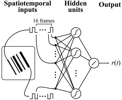
We trained two-layer neural networks with a tapped-delay line architecture (Fig. 1). There were 256 inputs, representing the spatiotemporal luminance signals S1(t), S1(t − 1), … , S1(t − 15), … , S16(t − 15), where the subscripts index the spatial positions of the bars, and t, … , t − 15 represent the 16 time delays in the temporal window (267 msec) preceding the response at time t. These luminance signals were represented as −1 (dark) and 1 (light). Each hidden unit had a hyperbolic tangent activation function tanh(x) ≡ (ex − e−x)/(ex + e−x). The output unit had a linear activation function and represented the instantaneous firing rate at time t. Thus the network transformed the spatiotemporal visual stimulus into a time-varying neuronal response. The network connections were initialized with Gaussian random numbers with zero mean and SD of 0.05 × d−1/2, where d represents the number of inputs to a particular layer. Bias terms for the hidden and output units were implemented by including an extra unit with a fixed value of 1. The connections from the bias units to the hidden and the output units were optimized with the other connections.
Figure 1.
Artificial neural network structure. (Left) One frame of the random-bar stimuli. The bias units are omitted for clarity.
Gradient descent was implemented with the back-propagation algorithm by using batch mode training (18). Briefly, the luminance stimuli were presented to the network, and the outputs were compared with the recorded responses. After each cycle through the training set, all of the network weights were adjusted to reduce the mean-square difference between the network output and the recorded response. To accelerate convergence, we used adaptive learning rates and added a momentum term to the weight updates (22). We also added a small decay term to each weight update (23) that drove weights that did not contribute to minimizing the error toward zero. Each connection weight was updated according to Δwi(t) = η∂E/∂wi + λΔwi(t − 1) − β sgn(wi(t − 1)), where wi is the weight of the ith connection in the network, η is the learning rate, ∂E/∂wi is the gradient of the error function computed by back-propagation (18), λ is the momentum (set to 0.7), β is the weight decay (set between 0.0001–0.001), and sgn(x) = 1 for x ≥ 0 and sgn(x) = −1 for x < 0.
The recorded stimulus–response data for each cell were partitioned into three nonoverlapping sets. The training data consisted of 24,576 stimulus–response pairs (≈7 min). A validation set with 4,095 pairs (≈1 min) was used to determine when training was stopped. Training was terminated when the mean-square error of the validation set exceeded the averaged error of the past 25 iterations. This method of early stopping minimizes overfitting on the training data (24). Most networks reached the termination point at between 200 and 1,500 iterations. A minimum of five networks were trained for each cell by using different initial conditions, and the network giving the minimum error for the validation set was selected as the final model. In some cases, a few networks performed similarly well in predicting the neuronal responses, and we noticed that they always showed similar hidden-unit RFs. We used a third test data set (4,096 pairs, ≈1 min) to evaluate the network performance.
To determine the proper number of hidden units for the networks, we modeled a subset of complex cells (n = 10) by using networks with one, four, and eight hidden units. The mean correlation coefficients for the test data were 0.28, 0.35, and 0.34 for one, four, and eight hidden units, and the performance of the networks with eight hidden units was not significantly different from that with four hidden units (P > 0.40). Thus for all of the cells used in this study, we used four hidden units for the initial network.
Because networks trained with the gradient descent algorithm can be trapped in local minima, they may have failed to capture some of the response properties. We therefore trained a second network on the residuals (the difference between the network prediction and the actual response) of the best network attained using the original firing rate. These residual networks had the same structure and inputs as the initial networks. The final network model for the cell was taken as the sum of the two networks giving the minimum error on the validation data. This combined network is functionally equivalent to a single network with eight hidden units. Empirically, however, training the two networks sequentially consistently provided a better fit of the data than training a single network with eight hidden units.
To determine the number of significant hidden units used by the network, we computed the mean-square error of the validation data after eliminating each possible combination of the hidden units. The number of significant hidden units was determined as the minimal combination that reduced the error to within 5% of the reduction attained by the full network.
Results
Predicting Cortical Responses to Random-Bar Stimuli.
We measured responses of simple and complex cells in the striate cortex of anesthetized cats. The stimulus consisted of 16 bars along the preferred orientation of the cell. Each bar varied randomly between light and dark over time. A neural network (Fig. 1) was trained to predict the response of each neuron to the random-bar stimuli (see Methods). After training, we tested the performance of the network using a data set that was not used in training.
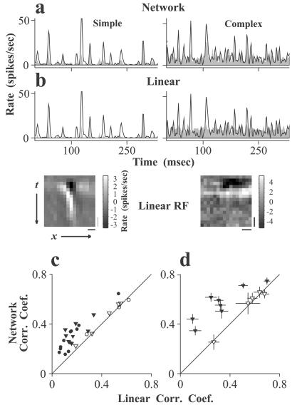
Fig. 2a shows the comparisons between the actual neuronal responses and the predictions by the networks for a simple and a complex cell. For both cell types, the networks captured well the temporal features in the responses, although they had a tendency to underestimate responses at high amplitudes (see Discussion). To further evaluate the performance of the network method, we compared it with the linear method that has been used previously to predict the responses of sensory neurons (7–9). We estimated the spatiotemporal receptive field (STRF) of each cell (Fig. 2b Lower) by averaging the stimulus preceding each spike (5, 25) using the training data set. The response of the cell to new stimuli (test data) was predicted as the convolution of the visual stimuli with the estimated linear RF followed by a halfwave rectification, with a threshold and a scaling factor as free parameters (Fig. 2b Upper). Fig. 2c summarizes the performance of the networks versus that of the linear method for 8 simple and 21 complex cells, measured by the correlation coefficients between the predicted and the actual responses (averaged over three to nine repeats of a 1-min stimulus sequence, mean = 4). The mean correlation coefficients for the simple cells were 0.45 (network) versus 0.44 (linear), and those for the complex cells were 0.31 (network) versus 0.17 (linear). Because the actual responses were averaged from small numbers of repeats, the performance of both methods is significantly underestimated by these correlation coefficients because of variability in the responses. To obtain a better measure of the performance of these methods, we recorded the responses of a subset of the neurons (five simple and eight complex cells) to 40 repeats of a short stimulus sequence (9 sec). For these response data (Fig. 2d), the mean correlation coefficients for the simple cells were 0.54 (network) versus 0.54 (linear), and those for the complex cells were 0.56 (network) versus 0.33 (linear). For all of the simple cells, the performance of the networks was not significantly different from that of the linear method (P > 0.10). For most of the complex cells (seven of eight), on the other hand, the network performed significantly better than the linear method (P < 0.001), indicating that the networks learned significant aspects of the nonlinear response properties of the complex cells.
Figure 2.
Predicting cortical responses to the random-bar stimuli. (a) Comparison between the actual responses of a simple and a complex cell with the network predictions. Line: actual responses averaged from 40 repeats of the stimulus; shaded: predicted responses. (b) Comparison between the actual responses (line) with the predictions (shaded) by the linear method. (Lower) Linear RFs of the cells computed with reverse correlation (5, 25). (Bars: vertical, 50 msec; horizontal, 1°) (c) Correlation coefficients between the predicted and the actual responses for the networks vs. those for the linear method, for 8 simple (open) and 21 complex (solid) cells. Triangles: cells used in d. (d) Correlation coefficients between the predicted and the actual responses (averaged from 40 repeats) for a subset of cells (triangles) in c. [Error bars: ± SE, estimated using a nonparametric bootstrap (44).] The correlation coefficient between the actual responses averaged from different repeats (20 repeats each) was 0.81 for complex cells and 0.87 for simple cells.
Connections in the Networks Modeling Simple Cells.
Although the structure of a feed-forward neural network differs from the visual cortical circuitry, the connection patterns in the trained networks may reveal the functional nature of the stimulus–response transformation performed by cortical neurons. For each hidden unit of a trained network, we examined its connections with all of the input units, which represents the STRF for that hidden unit.
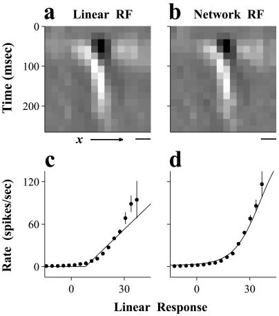
For a simple cell, only one to three (mean = two) of the eight hidden units contributed significantly to predicting the responses. The RFs of these significant hidden units had spatially separate ON and OFF subregions (Fig. 3b). These RFs were nearly identical to the linear RF of the cell (Fig. 3a), indicating that the network approximated the responses of simple cells in a manner similar to the linear method. To gain a better understanding of how both methods predicted the simple cell responses, we plotted the firing rate of each cell versus the convolution of the stimuli with its RF (Fig. 3 c and d, dots). This convolution can be thought of as the intracellular response of the cell, which has an approximately linear relationship with the stimulus (26). The firing rate of the cell as a function of this linear response showed a nonlinear monotonic increase, which presumably reflects the relationship between the firing rate of the cell and its intracellular response. In the linear method, a halfwave rectification was used to approximate this nonlinear relationship (Fig. 3c, line), whereas in the neural network, the hidden-unit activation function was used (Fig. 3d, line). When the actual responses were fit with a half-power function y(x) = βmax(x, 0)γ (where x and y represent the result of the convolution and the firing rate, respectively, and β and γ are free parameters), the mean exponent (γ) of the simple cells was 2.1 ± 0.6 (n = 8, mean ± SD), similar to that measured by Anzai et al. (27) in the visual cortex of the cat.
Figure 3.
Analysis of a network representing a simple cell. (a) Linear STRF of the simple cell. (b) STRF of the significant hidden unit of the network. Luminance indicates the sign and strength of the connection from each input unit. (horizontal bar, 1°) (c) Firing rate of the neuron (dots: mean; bars: ± SE) vs. the linear response and the approximation of this function by the linear method (line). (d) Firing rate of the neuron vs. the linear response of the significant hidden unit, and approximation of this function by the hidden-unit activation function (line).
Connections in Networks Modeling Complex Cells.
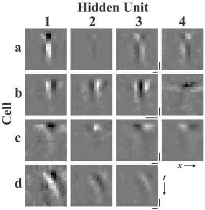
The trained network for each complex cell had two to six hidden units (mean = 3.8) that contributed significantly to predicting the neuronal responses. The RFs of these hidden units had segregated ON and OFF subregions that evolved smoothly over time (Fig. 4), resembling the RFs of simple cells (Fig. 3a). These hidden-unit RFs differed from the linear RFs of the complex cells, most of which did not show spatial segregation of ON and OFF subregions (Fig. 2b Lower). The RFs of different hidden units exhibited similar spatial frequencies but different phases, indicating that the networks used several distinct subunits to simulate the responses of complex cells.
Figure 4.
Hidden-unit RFs of networks representing four complex cells (a–d). To show the contribution of each hidden unit to the network output, these RFs are scaled by the connection weights from the corresponding hidden units to the output unit. Only the most significant hidden units are plotted. (Bar: vertical, 50 msec; horizontal, 1°)
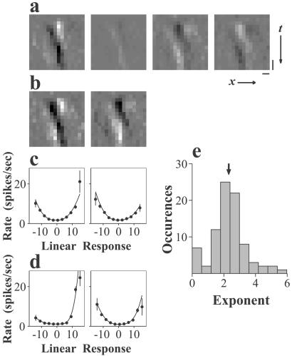
The RFs of some hidden units had similar spatiotemporal profiles and differed only in the sign and amplitude of their responses (e.g., units 3 and 4 of Cell a, units 3 and 4 of Cell c; Fig. 4), suggesting redundancy among different hidden units. To further simplify the network models, we performed a principal component analysis of all of the significant hidden units of each network (Fig. 5a), yielding a set of linearly independent principal components that together account for all of the variance in the hidden-unit RFs. For each network simulating a complex cell, one to three principal components (mean = 2.1) were sufficient to account for >95% of the variance (Fig. 5b). These significant principal components always showed similar numbers of ON/OFF subregions and temporal dynamics as the original hidden-unit RFs but had different spatial phases.
Figure 5.
Decomposing hidden-unit RFs. (a) RFs of the four significant hidden units of the network representing a complex cell. (Bars: vertical, 50 msec; horizontal, 1°.) (b) The two most significant principal components. (c) Firing rate of the neuron vs. the linear response of each principal components (dots: mean; vertical lines: ± SE). The solid curve shows the fit of the data with half-power functions. (d) Same as c, for a different cell. (e) Summary of the exponents of the fits (n = 84). Arrow indicates the mean.
To understand how these principal components contribute to the responses of complex cells, we plotted the firing rate of each complex cell against the convolution of the stimuli with each of the significant principal components (Fig. 5 c and d). Most of these functions were bimodal, clearly distinct from the monotonic functions seen for simple cells (Fig. 3c). However, both the left and the right halves of the functions showed an expansive nonlinearity similar to that for simple cells. To quantify this nonlinearity, we fit the left and the right halves of these functions separately with a power function y(x) = β|x|γ, where x and y represent the result of the convolution and the firing rate respectively, and β and γ are free parameters. The mean exponent (γ) obtained was 2.3 with a standard deviation of 1.1 (Fig. 5e), similar to that measured for simple cells (27, 28) (see above). The majority of the bimodal functions seen in our population of complex cells were asymmetric because of different gain parameters (β) for the left and right halves. In summary, each bimodal function can be treated as the sum of two half-power functions, each representing the contribution of a subunit, the RF of which is either the same as the principal component or opposite in sign from it. When we predicted the firing rate of each neuron by using linear summation of the responses of the significant principal components after transformation by their corresponding bimodal functions, the results were not significantly different from those of the neural networks (P = 0.64, Wilcoxon signed rank test). These results indicate that the response of a complex cell to the random-bar stimuli can be approximated as the sum of a small number of simple-cell-like subunits.
Generalization of the Model: Predicting Direction Selectivity.
It is important to know whether the current model, which was developed on the basis of responses to the random-bar stimuli, can be used to predict responses to other types of stimuli. In some networks, the locations of the ON and OFF subregions in the hidden-unit RFs shifted progressively over time (Fig. 4, Cell d; Fig. 5a), suggesting direction selectivity in these cells. Previous studies have shown that direction selectivity of simple cells can be predicted from their linear STRFs and the expansive nonlinearity in their responses (4, 28). Here, because the response of a complex cell can be approximated as the sum of several subunits, we could predict the direction selectivity of the cell by using the RFs of these subunits and their expansive nonlinearities.
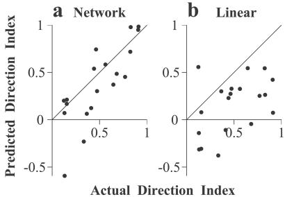
For 19 of the 21 complex cells, we recorded the responses to full-contrast sinusoidal gratings at the optimal orientation, drifting at the preferred and nonpreferred directions. For each cell, we computed the direction index as (Rp − Rn)/(Rp + Rn), where Rp and Rn are the responses at the preferred and the nonpreferred directions. We then predicted the direction index from the network-derived model. First, we performed a spatiotemporal Fourier transform of the RF of each subunit. The linear responses of each subunit to the preferred and the nonpreferred drifting gratings were obtained from the amplitude and the phase spectra of the Fourier transform at the spatiotemporal frequency, where the actual direction index was measured. Second, these linear responses were passed through the half-power nonlinearities with the corresponding exponents. Finally, the direction index of each cell was predicted after summing the contributions of all of the subunits. For the majority of cells, the predictions agreed well with the direction selectivity measured with drifting gratings (Fig. 6a). The mean of the actual direction index was 0.49, and that of the predicted direction index was 0.38. The correlation coefficient between the predicted and the actual indices was 0.80. We also predicted the direction index by using the linear RF of each complex cell (Fig. 6b, mean direction index = 0.15, correlation coefficient = 0.47). Compared with the linear model, the network-derived models performed significantly better (P < 0.05). Thus, the stimulus–response relationship of the complex cells extracted from their responses to the random-bar stimuli was general in that it could predict a response property measured with a different type of stimulus. Note that although the predictions of the linear models were worse than those of the network-derived models, they were significantly better than random (P < 0.05), indicating that the linear RFs contained some information about the direction selectivity of the complex cells.
Figure 6.
Predicting direction selectivity of complex cells. (a) The direction index predicted based on the principal components vs. the actual direction index. (b) The direction index predicted based on the linear RFs vs. the actual direction index.
Discussion
Several circuitry models have been proposed to account for the response properties of complex cells. A main feature that distinguishes complex from simple cells is that the response of a complex cell is insensitive to the contrast-polarity (light or dark) and stimulus position within the RF. This insensitivity may result from convergence of multiple simple cells whose RFs have different ON/OFF locations (1, 29), from nonlinear integration of thalamic inputs by the active dendrites of pyramidal neurons (30), or from recurrent excitation between cortical cells with different ON/OFF locations (31). We have shown that the responses of complex cells to the random-bar stimuli can be approximated by the sum of a small number of computational subunits. However, it is important to note that each network model provides a functional description of the input–output relationship of a complex cell rather than a mechanistic model for the underlying neuronal circuitry. Although the RF of each subunit resembles that of a simple cell along the axis perpendicular to the preferred orientation of the cell (4, 32), each subunit does not necessarily correspond to an actual simple cell in the cortex.
In principle, a two-layer feed-forward neural network can be trained to approximate any input–output transfer function given a sufficient number of hidden units (33, 34). An important question is whether the optimized connection weights exhibit features that provide insights into the nature of the stimulus-response transformation. Here, the networks consistently simulated the responses of complex cells by combining small numbers of simple-cell-like hidden units, indicating that such a structure is especially well suited for approximating the responses to the type of spatiotemporal stimuli we have used. Lehky et al. (16) trained feed-forward networks to simulate the responses of complex cells in monkey V1 to a variety of two-dimensional static spatial patterns. These networks predicted very well the total number of spikes in response to each pattern, but their hidden units had more complex RFs, many of which did not resemble RFs of simple cells. The difference between the results of the previous and the present studies may be due to the difference in the number of hidden units in the networks, the amount of data used in training, or whether the networks took into account the temporal dynamics of the responses. Another possibility is that the two-dimensional spatial stimuli used in the previous study evoked more complex responses than did the random-bar stimuli.
The networks extracted the stimulus–response transformation of complex cells, assuming only that this transformation could be approximated by a two-layer network with a finite number of hidden units. Interestingly, the trained networks performed an operation similar to that of the energy model (19, 35), in which a complex cell is described as the sum of four halfwave rectified and squared linear filters (36, 37). The energy model has been used to explain the responses of complex cells to two-bar stimuli (11, 38) and to drifting and contrast-reversing gratings (11, 39). It predicts a bimodal (squaring) relationship between the neuronal firing rate and the linear response of the underlying filter similar to what we have observed for the principal components (Fig. 5 c and d). However, there are quantitative differences. First, the exponents measured for the subunits in our models had a broad distribution (Fig. 5e), whereas in an ideal energy model, these exponents have a fixed value of 2. Second, the different subunits often contributed unequally to the response of the cell, as indicated by the asymmetry between the left and the right halves of the bimodal functions (e.g., Fig. 5d Left). To evaluate the significance of these deviations from the energy model in fitting the responses of complex cells, we predicted the response of each cell by summing the squared response of each subunit with equal weight. The mean correlation coefficient between the predicted and the actual responses was 0.23, which was lower than that using the network model (correlation coefficient = 0.31). This difference indicates that the deviations from the ideal energy model have a significant effect on the performance of the models. For most of the complex cells in our sample, we observed linear RFs (Fig. 2b) that contributed significantly to the neuronal responses, as indicated by the fact that they can partially predict the random-bar responses and direction selectivity of these cells (Figs. 2 c and d and 6b). Linear RFs are not predicted by the energy model but can be explained by the unequal contributions of the different subunits.
The network models did not capture the full input–output relationship of the complex cells, because the correlation coefficient between the predicted and the actual responses was significantly less than 1. Several factors may have affected the network performance. First, the hidden-unit activation function may not fully capture the expansive nonlinearity in the neuronal responses, which may be why the networks underestimate the responses at high amplitudes (Fig. 2a). However, this factor alone could not account for most of the errors in the model, because predicting the responses by using the best fitted half-power function of each subunit did not significantly improve the prediction (see above). Second, the networks predicted the responses on the basis of stimuli within a window of 267 msec, which could not account for adaptation occurring at longer time scales (40, 41) or nonstationarity in the data. Finally, there may exist more complex nonlinearities, such as contrast normalization (28, 37) or the modulation of responses by stimuli in the nonclassical RFs (42). Such modulation may result from the activity of a large number of neighboring cells (37), the representation of which would require many more hidden units in the network. Future models incorporating these nonlinearities may improve the prediction of responses of both simple and complex cells.
In this study, we have used visual stimuli that were modulated along one spatial dimension. However, the neural network method can be used to analyze the responses to two-dimensional visual stimuli, which may reveal more complex cortical response properties. Furthermore, because this method does not require inputs with specific statistical properties, it can be used to analyze responses to inputs with complicated statistics such as natural scenes and may thus have a wider applicability than other nonlinear techniques such as the Wiener kernel approach (43). Unlike the conventional approach using specialized stimuli to probe a particular response property, the networks can be trained on arbitrarily large ensembles of stimulus–response data, requiring far fewer assumptions about which features of the stimuli are relevant to the cell. Thus this method may be well suited for the study of higher cortical areas in which neuronal properties are more complex and poorly understood.
Acknowledgments
We thank Kathleen Bradley, Gidon Felsen, and Timothy Kubow for helpful discussions. This work was supported by grants from National Eye Institute (R01 EY12561-01), National Science Foundation (IBN-9975646), and the Office of Naval Research (N00014-00-1-0053).
Abbreviations
- RF
receptive field
- STRF
spatiotemporal receptive field
References
- 1.Hubel D H, Wiesel T N. J Physiol. 1962;160:106–154. doi: 10.1113/jphysiol.1962.sp006837. [DOI] [PMC free article] [PubMed] [Google Scholar]
- 2.Campbell F W, Cleland B G, Cooper G F, Enroth-Cugell C. J Physiol (London) 1968;198:237–250. doi: 10.1113/jphysiol.1968.sp008604. [DOI] [PMC free article] [PubMed] [Google Scholar]
- 3.Eggermont J J, Johannesma P M, Aertsen A M. Q Rev Biophys. 1983;16:341–414. doi: 10.1017/s0033583500005126. [DOI] [PubMed] [Google Scholar]
- 4.DeAngelis G C, Ohzawa I, Freeman R D. J Neurophysiol. 1993;69:1118–1135. doi: 10.1152/jn.1993.69.4.1118. [DOI] [PubMed] [Google Scholar]
- 5.Reid R C, Victor J D, Shapley R M. Visual Neurosci. 1997;14:1015–1027. doi: 10.1017/s0952523800011743. [DOI] [PubMed] [Google Scholar]
- 6.DiCarlo J J, Johnson K O, Hsiao S S. J Neurosci. 1998;18:2626–2645. doi: 10.1523/JNEUROSCI.18-07-02626.1998. [DOI] [PMC free article] [PubMed] [Google Scholar]
- 7.Eggermont J J, Aertsen A M, Johannesma P I. Hear Res. 1983;10:191–202. doi: 10.1016/0378-5955(83)90053-9. [DOI] [PubMed] [Google Scholar]
- 8.Dan Y, Atick J J, Reid R C. J Neurosci. 1996;16:3351–3362. doi: 10.1523/JNEUROSCI.16-10-03351.1996. [DOI] [PMC free article] [PubMed] [Google Scholar]
- 9.Theunissen F E, Sen K, Doupe A J. J Neurosci. 2000;20:2315–2331. doi: 10.1523/JNEUROSCI.20-06-02315.2000. [DOI] [PMC free article] [PubMed] [Google Scholar]
- 10.Movshon J A, Thompson I D, Tolhurst D J. J Physiol (London) 1978;283:53–77. doi: 10.1113/jphysiol.1978.sp012488. [DOI] [PMC free article] [PubMed] [Google Scholar]
- 11.Movshon J A, Thompson I D, Tolhurst D J. J Physiol (London) 1978;283:79–99. doi: 10.1113/jphysiol.1978.sp012489. [DOI] [PMC free article] [PubMed] [Google Scholar]
- 12.Hertz J, Krogh A, Palmer R G. Introduction to the Theory of Neural Computation. Redwood City, CA: Addison–Wesley; 1991. [Google Scholar]
- 13.Lehky S R, Sejnowski T J. Nature (London) 1988;333:452–454. doi: 10.1038/333452a0. [DOI] [PubMed] [Google Scholar]
- 14.Zipser D, Andersen R A. Nature (London) 1988;331:679–684. doi: 10.1038/331679a0. [DOI] [PubMed] [Google Scholar]
- 15.Lockery S R, Wittenberg G, Kristan W B, Jr, Cottrell G W. Nature (London) 1989;340:468–471. doi: 10.1038/340468a0. [DOI] [PubMed] [Google Scholar]
- 16.Lehky S R, Sejnowski T J, Desimone R. J Neurosci. 1992;12:3568–3581. doi: 10.1523/JNEUROSCI.12-09-03568.1992. [DOI] [PMC free article] [PubMed] [Google Scholar]
- 17.Bankes S C, Margoliash D. J Neurophysiol. 1993;69:980–991. doi: 10.1152/jn.1993.69.3.980. [DOI] [PubMed] [Google Scholar]
- 18.Rumelhart D E, Hinton G E, Williams R J. In: Parallel Distributed Processing. Rumelhart D E, McClelland J L, editors. Vol. 1. Cambridge, MA: MIT Press; 1986. pp. 318–362. [Google Scholar]
- 19.Adelson E H, Bergen J R. J Opt Soc Am A. 1985;2:284–299. doi: 10.1364/josaa.2.000284. [DOI] [PubMed] [Google Scholar]
- 20.Sutter E E. In: Advanced Methods of Physiological Systems Modeling. Marmarelis V Z, editor. Vol. 1. Los Angeles: Univ. of Southern California; 1987. pp. 303–315. [Google Scholar]
- 21.Skottun B C, De Valois R L, Grosof D H, Movshon J A, Albrecht D G, Bonds A B. Vision Res. 1991;31:1079–1086. doi: 10.1016/0042-6989(91)90033-2. [DOI] [PubMed] [Google Scholar]
- 22.Plaut D C, Nowlan S J, Hinton G E. Technical Report CMU-CS-86–126. Carnegie Mellon University, Pittsburgh: Department of Computer Science; 1986. [Google Scholar]
- 23.Ishikawa M. Neural Networks. 1996;9:509–521. [Google Scholar]
- 24.Sarle W S. Proc. 27th Symp. Comp. Sci. Stat. PA, June 21–24: Pittsburgh; 1995. pp. 352–360. [Google Scholar]
- 25.Jones J P, Palmer L A. J Neurophysiol. 1987;58:1187–1211. doi: 10.1152/jn.1987.58.6.1187. [DOI] [PubMed] [Google Scholar]
- 26.Jagadeesh B, Wheat H S, Kontsevich L L, Tyler C W, Ferster D. J Neurophysiol. 1997;78:2772–2789. doi: 10.1152/jn.1997.78.5.2772. [DOI] [PubMed] [Google Scholar]
- 27.Anzai A, Ohzawa I, Freeman R D. J Neurophysiol. 1999;82:891–908. doi: 10.1152/jn.1999.82.2.891. [DOI] [PubMed] [Google Scholar]
- 28.Albrecht D G, Geisler W S. Visual Neurosci. 1991;7:531–546. doi: 10.1017/s0952523800010336. [DOI] [PubMed] [Google Scholar]
- 29.Alonso J M, Martinez L M. Nat Neurosci. 1998;1:395–403. doi: 10.1038/1609. [DOI] [PubMed] [Google Scholar]
- 30.Mel B W, Ruderman D L, Archie K A. J Neurosci. 1998;18:4325–4334. doi: 10.1523/JNEUROSCI.18-11-04325.1998. [DOI] [PMC free article] [PubMed] [Google Scholar]
- 31.Chance F S, Nelson S B, Abbott L F. Nat Neurosci. 1999;2:277–282. doi: 10.1038/6381. [DOI] [PubMed] [Google Scholar]
- 32.McLean J, Raab S, Palmer L A. Visual Neurosci. 1994;11:271–294. doi: 10.1017/s0952523800001632. [DOI] [PubMed] [Google Scholar]
- 33.Hornik K, Stinchcombe M, White H. Neural Networks. 1989;2:359–366. [Google Scholar]
- 34.Cybenko G. Math Control Signals Systems. 1989;2:303–314. [Google Scholar]
- 35.Pollen D A, Gaska J P, Jacobson L D. In: Models of Brain Function. Cotterill R M J, editor. Cambridge, MA: Cambridge Univ. Press; 1989. pp. 115–135. [Google Scholar]
- 36.Heeger D J. In: Computational Models of Visual Processing. Landy M S, Movshon J A, editors. Cambridge, MA: MIT Press; 1991. pp. 119–133. [Google Scholar]
- 37.Heeger D J. Visual Neurosci. 1992;9:181–197. doi: 10.1017/s0952523800009640. [DOI] [PubMed] [Google Scholar]
- 38.Emerson R C, Bergen J R, Adelson E H. Vision Res. 1992;32:203–218. doi: 10.1016/0042-6989(92)90130-b. [DOI] [PubMed] [Google Scholar]
- 39.Maffei L, Fiorentini A. Vision Res. 1973;13:1255–1267. doi: 10.1016/0042-6989(73)90201-0. [DOI] [PubMed] [Google Scholar]
- 40.Maffei L, Fiorentini A, Bisti S. Science. 1973;182:1036–1038. doi: 10.1126/science.182.4116.1036. [DOI] [PubMed] [Google Scholar]
- 41.Müller J R, Metha A B, Krauskopf J, Lennie P. Science. 1999;285:1405–1408. doi: 10.1126/science.285.5432.1405. [DOI] [PubMed] [Google Scholar]
- 42.Allman J, Miezin F, McGuinness E. Annu Rev Neurosci. 1985;8:407–430. doi: 10.1146/annurev.ne.08.030185.002203. [DOI] [PubMed] [Google Scholar]
- 43.Wiener N. Nonlinear Problems in Random Theory. New York: Technology Press of MIT and Wiley; 1958. [Google Scholar]
- 44.Efron B, Tibshirani R J. An Introduction to the Bootstrap. New York: Chapman & Hall; 1993. [Google Scholar]


