Modelling behavioural changes and vaccination in the transmission of respiratory viruses with co–infection

Abstract

We consider a mathematical model to explore the effects of human behavioural changes on the transmission of two respiratory viruses, where co–infection is possible. The model includes an index to describe the human choices induced by information and rumours regarding the diseases. We first consider the case in which the public health authorities rely only on non–pharmaceutical containment measures and perform a qualitative analysis of the model through bifurcation theory, in order to analyse the existence and stability of both endemic and co–endemic equilibria. We also show the impact of the most relevant information–related parameters on the system dynamics. Then, we extend the model by assuming that a vaccine is available for each of the two viruses. We show how adherence to social distancing may be affected by information and rumours regarding the vaccination coverage in the community. Finally, we investigate the effects of seasonality by introducing a two–state switch function to represent a reduction in both vaccination and transmission rates during the summer season. We found that seasonality causes an increase in the prevalence peaks, suggesting that the detrimental effects due to the reduction of vaccination rates prevail over the beneficial ones due to the reduction of transmission.

Introduction

A co–infection between two respiratory viruses is defined as the simultaneous infection of an individual with two genetically different viruses that infect the respiratory system (Cox 2001). This phenomenon can involve influenza or parainfluenza viruses, coronaviruses (e.g., MERS–CoV, SARS–CoV–2), adenoviruses, respiratory syncytial virus (RSV) and human rhinoviruses (HRV). Co–infection can occur between viruses belonging to different species or also between different strains of the same virus (Cox 2001). The interaction between two different viruses can be classified into two categories: positive interaction, when the two viruses act together worsening the symptoms and outcome of the disease, and negative interaction, when the presence of one virus inhibits the replication of the other virus in the host’s body (Devi et al. 2021). Implications of positive interactions between Influenza A virus (IAV) and SARS–CoV–2 include enhanced host infectivity (Bai et al. 2021) as well as greater body weight loss and more severe lung damage in co–infected hamsters (Kinoshita et al. 2021). As for negative interactions, one of the most common mechanisms of negative viral-viral interaction is viral interference, which occurs when the presence of one virus (the interfering one) in a host inhibits the replication or activity of another virus (Wu et al. 2020). Several couples of respiratory viruses have this particular feature, e.g., HRV and IAV, HRV and RSV, HRV and SARS–CoV–2 (Piret and Boivin 2022).

Another relevant aspect about co–infections is that when two different viruses or two different strains of the same virus infect a host, they can gain new properties through phenomena like recombination and reassortment (Bolze et al. 2022; Zhang and Cao 2014). Recombination is defined as the exchange of genetic segments between two viral genomes which co-infect the same host cell. Reassortment is a particular type of recombination and concerns viruses with segmented genomes. It occurs when the two viruses swap complete genome segments, giving rise to new segment combinations (Pérez-Losada et al. 2015).

Since the onset of the COVID–19 pandemic, several studies have investigated the frequency of co–infections with SARS–CoV–2 (Dadashi et al. 2021; Krumbein et al. 2023; Dao et al. 2021; Yan et al. 2023). The proportion of co–infected individuals can vary significantly depending on several factors including the season, the geographical region, age group, sex and health status. Dadashi et al. (2021) performed a systematic review of papers published from December 2019 to September 2020, finding an overall influenza prevalence of 0.8% in confirmed cases of COVID–19. In 2023, Krumbein et al. (2023) conducted a meta–analysis to determine the proportion of co–infections with any respiratory virus between SARS–CoV–2 patients to identify the most frequent co-pathogens and to compare the clinical outcomes. They found that the most common co-pathogens are influenza virus (1.54%) and enteroviruses (1.32%). Furthermore, co–infected patients are significantly more exposed to the risk of death than patients infected only with SARS–CoV–2. Similar estimates were obtained by Dao et al. (2021) and Yan et al. (2023). The latter study also shows that co–infected have a higher probability of developing severe outcomes when compared with mono–infected patients. In addition, the co–infection proportion is significantly high in dead patients (36.67%).

Overall, although the proportion of co–infections is generally low, co–infections may have a relevant impact on the course of epidemic outbreaks in terms of both the disease burden and their potential ability to generate new variants or entirely new viruses with unknown impact on transmissibility and disease severity (Bolze et al. 2022). Consequently, it is essential to conduct further research into the underlying mechanisms of the phenomenon and the possible consequences of co–infections on the population. Mathematical modelling may provide useful tools to assess the dynamics of respiratory virus co–infection and to provide information to public health practitioners regarding the implementation of pharmaceutical and non–pharmaceutical mitigation strategies (Majeed et al. 2023; Fahlena et al. 2022).

In the last few years, and especially after the COVID–19 global pandemic, mathematical models designed to investigate respiratory viruses co–infection dynamics began to catch the attention of scholars. Several intriguing models and analyses can be found in the recent literature. In 2013, Zhang et al. developed a SIR (Susceptible–Infectious–Removed) compartmental model including two strains of influenza virus (Zhang et al. 2013). Their model takes into account co–infection as well as reassortment. Pinky et al. proposed a co–infection model where an influenza–like virus blocks infection with SARS–CoV–2 (Pinky and Dobrovolny 2022). More recently, Bhowmick et al. considered SARS–CoV–2 and influenza–like viruses (ILI) co–infection and incorporated the saturated treatment rate to evaluate the impact of limited treatment resources on the time evolution of the epidemic (Bhowmick et al. 2023). In their model, it is assumed that direct co–infection is possible, that is susceptible individuals may become infected simultaneously with SARS–CoV–2 and ILI. However, there is no evidence that direct co–infection is particularly likely to occur, therefore it is usually neglected when modelling co–infections (Hamelin et al. 2019). Direct co–infection is not considered by Fahlena et al. (2022), who introduced a SIR–like compartmental model designed to describe the interaction of two generic respiratory viruses. Their model has the advantage of being detailed, mathematically tractable and sufficiently general to be applied both in the case of positive and negative interaction between respiratory viruses.

All the aforementioned models can provide useful insights into the co–infection dynamics. However, they do not consider an important aspect, namely the human behavioural changes and their effects on the course of the epidemic. Indeed, it is widely acknowledged that human behaviour is a key determinant of the effectiveness of mitigation strategies during an epidemic, especially when the adoption of self–protective measures is based essentially on free will (Bergstrom and Hanage 2024; Lewnard and Lo 2020; West et al. 2020). Information and rumours about the spread of the disease may be a critical factor as to whether or not the individuals adopt protective measures, like social distancing, wearing masks, vaccination, and so on (Collinson et al. 2015; Wang et al. 2016). During the recent COVID–19 pandemic, it has been clear that social distancing, together with vaccines and pharmacological treatments is essential to mitigate the disease (Khataee et al. 2021; Zhou et al. 2020). However, in some cases, people did not adhere to these measures due to various reasons, such as the perceived high risk of vaccine side effects or the perceived low risk of infection due to low prevalence or high vaccination coverage. These behaviours have posed additional problems for the public health systems (Masters et al. 2020; Troiano and Nardi 2021; Dror et al. 2020). This example underscores the crucial role of information–dependent behavioural changes in both mitigating and fuelling epidemics.

Motivated by the above–mentioned considerations, we consider in this paper a mathematical model for co–infections of respiratory viruses that takes into account information–dependent human behavioural changes. We use the SIR–like model proposed by Fahlena et al. (2022) as baseline model and augment it with the information index, a state variable defined by a distributed–delay equation. Such an index was introduced in 2007 by A. d’Onofrio and P. Manfredi to describe the information–induced perception regarding the status of the disease (Manfredi and d’Onofrio 2013; d’Onofrio et al. 2007) and is nowadays a consolidated tool in the field of Behavioural Epidemiology of Infectious Diseases (BEID) (Manfredi and d’Onofrio 2013; Wang et al. 2016).

Firstly, we consider the case in which the public health authorities rely only on non–pharmaceutical containment measures that reduce contact patterns (e.g., social distancing). Assuming an exponentially fading memory kernel, we derive a system of non–linear ordinary differential equations. We conduct a qualitative analysis using stability and bifurcation theory, emphasizing both the role of the control reproduction number, ${\mathcal{R}}_C$, and the invasion numbers of the two viruses. In particular, we show that the disease–free equilibrium destabilises at ${\mathcal{R}}_C=1$ via a transcritical forward bifurcation; in addition, we give sufficient conditions for the existence of locally stable co–endemic equilibria by proving the existence of a forward bifurcation when the minimum between the two invasion numbers crosses the threshold value of 1. Through numerical simulations, we also show the impact of the most relevant information–related parameters on the system dynamics.

Secondly, we extend the model by assuming that a vaccine is available for each of the two viruses. For each of them, the vaccination choice is assumed to be partially voluntary and dependent on information about the spread of the disease in both the present and recent past. We show how adherence to social distancing may be affected by the information and rumours concerning the vaccination coverage in the community.

Finally, we numerically show the effects of seasonality on the course of epidemics. In fact, many respiratory viral diseases exhibit a seasonal pattern, with outbreaks often peaking during certain times of the year (Moriyama et al. 2020). The seasonality may be caused by several factors, including environmental conditions and human behaviour (Neumann and Kawaoka 2022). We include seasonality in the model by considering reduced vaccination and transmission rates in the summer season.

The rest of the paper is organized as follows: the model is introduced in Section 2. In Section 3, the control reproduction numbers and the invasion numbers are computed. Moreover, the existence and stability of the equilibria are established, and the occurrence of transcritical bifurcations is shown. In Section 4, we investigate through numerical simulations how human behavioural changes affect the dynamics of the model. In Section 5, we generalise the model by considering both information–induced vaccination and vaccination–induced relaxation of non–pharmaceutical containment measures. We discuss the main results and give an outlook on possible research perspectives in Section 6.

The model

State variables and the information index

Let us consider two generic respiratory viruses, named virus–1 and virus–2. We assume that the total population is divided into seven disjointed compartments: susceptible (S), infected only by virus–1 ($I_1$), infected only by virus–2 ($I_2$), co–infected ($I_3$), recovered only from virus–1 ($R_1$), recovered only from virus–2 ($R_2)$ and recovered from co–infection ($R_3$). The size of each compartment at time t represents a state variable of the model. The size of the total population at time t, denoted by N(t), is given by:

$$\begin{array}{c}\hfill N(t)=S(t)+\sum _{i=1}^3{I}_i(t)+\sum _{i=1}^3{R}_i(t).\end{array}$$

In order to model the effects of information–dependent behavioural changes, we assume that the individual choice to use disease–protective devices is partially voluntary and depends on the available information about the spread of the disease in the community. Information is mathematically modelled by the information index M(t), which contains information about the current and past values of the diseases and is defined as the follows (d’Onofrio et al. 2007; d’Onofrio and Manfredi 2009):

$$\begin{array}{c}\hfill M(t)={\int }_0^{+\infty }g(I_1(t-\tau ),I_2(t-\tau ),I_3(t-\tau )){\text{Erl}}_{1,a}(\tau )d\tau .\end{array}$$ 1

In the latter expression, g is called message function and ${\text{Erl}}_{1,a}$ denotes the first–order Erlang distribution kernel (also known as exponentially fading kernel), i.e.:

$$\begin{array}{c}\hfill {\text{Erl}}_{1,a}(\tau )=a{e}^{-a\tau },\tau \in {\mathbb{R}}^{+},\end{array}$$ 2

where the constant $a\in {\mathbb{R}}^{+}$ is the rate parameter of the distribution.

As for the message function g, it describes the information that influences the individual’s choice to adopt or not to adopt self–protective measures. We consider the following function:

$$\begin{array}{c}\hfill g(I_1,I_2,I_3)=k_1{I}_1+k_2{I}_2+k_3{I}_3.\end{array}$$ 3

Here, the term $k_i{I}_i$, for $i=1,2,3,$ defines the perceived risk of infection, which is assumed to be proportional to the infection prevalence $I_i$ (Wang et al. 2016). The parameter $k_i\in [0,1]$, for $i=1,2,3,$ is the information coverage regarding the infected by virus–1, virus–2 and both viruses, respectively. Such parameter represents the balance between two different processes: the disease under-reporting – here assumed to be the prevailing process – due mainly to routine procedures, and the overestimation usually induced by media and rumours on the disease status (Buonomo et al. 2008).

Modelling the transmission rates

Let us denote by $a_1$ (resp. $a_2$) the transmission rate of virus–1 (resp. virus–2), and by ${\pi }_1$ (resp. ${\pi }_2$) the probability of successful infection after contact with an individual infected by virus–1 (resp. virus–2). Moreover, denote by $a_3$ the rate at which co–infected individuals transmit one of the two viruses and let ${\pi }_3$ be the corresponding probability of successful infection. Finally, denote by $a_4$ the co–infection rate, i.e., the rate at which the individuals infected from one virus also contract the other virus and let ${\pi }_4$ be the corresponding probability of successful infection.

We assume that the public health system enacts campaigns to encourage the reduction of interpersonal contacts (e.g., social distancing, wearing masks, etc.). The individual’s compliance with the recommendations is assumed to depend partially on the information about the spread of the disease in both the present and recent past. Since every transmission rate can be seen as the product of the contact rate times the probability of getting infected after contact with an infectious individual, we assume that the contact rate depends on the information index M(t). We set:

$$\begin{array}{c}\hfill a_j(M)={\pi }_j[\widehat{c}-c_0-c_1(M)],j=1,\cdots ,4,\end{array}$$ 4

where $\widehat{c}$ is the “baseline” contact rate (i.e., the contact rate when no reduction strategy is in place), $c_0$ is the information–independent reduction rate due to compliance with public health policies and $c_1(M)$ is the rate of reduction in interpersonal contacts due to information–dependent voluntary compliance with governmental policies. The function $c_1$ is assumed to be increasing with M, $c_1(0)=0$, and $\widehat{c}>c_0+\text{max}(c_1(M))$. The last inequality guarantees that $a_j(M)$ is positive for all values of M.

Equation (4) may be rewritten as:

$$\begin{array}{c}\hfill a_j(M)={\widehat{a}}_j-a_{j,0}-a_{j,1}(M),\end{array}$$ 5

where ${\widehat{a}}_j={\pi }_j\widehat{c}$, $a_{j,0}={\pi }_j{c}_0$ and $a_{j,1}(M)={\pi }_j{c}_1(M)$. A specific form of $a_{j,1}(M)$ will be given in subsection 2.4.

The balance equations

The balance equations for the seven compartments S(t), $I_i(t)$ and $R_i(t)$, for $i=1,2,3$ are illustrated in the flowchart in Figure 1. As mentioned above, the model structure follows the framework introduced by Fahlena et al. (2022), in which disease-induced mortality is neglected and the total population size is assumed to be constantly equal to its initial value. In our formulation, we extend this model by introducing the human behavioural changes through the information index (1) – (3) and the information–dependent rates $a_1,a_2,a_3$ and $a_4$ defined in (5). We get the following system of non–linear ordinary differential equations:

$$\begin{array}{cc}\hfill \dot{S}(t)& =\mu -a_1(M)S{I}_1-a_2(M)S{I}_2-a_3(M)S{I}_3+{\rho }_1{R}_1\hfill \\ \hfill & +{\rho }_2{R}_2+{\rho }_3{R}_3-\mu S,\hfill \end{array}$$ 6a

$$\begin{array}{cc}\hfill \dot{I_1}(t)& =a_1(M)S{I}_1+p{a}_3(M)S{I}_3-{\gamma }_1{I}_1+a_1(M)R_2{I}_1\hfill \\ \hfill & +a_3(M)R_2{I}_3-q{a}_4(M)I_1{I}_2-a_4(M)I_1{I}_3-\mu I_1,\hfill \end{array}$$ 6b

$$\begin{array}{cc}\hfill {\dot{I}}_2(t)& =a_2(M)S{I}_2+(1-p)a_3(M)S{I}_3-{\gamma }_2{I}_2+a_2(M)R_1{I}_2\hfill \\ \hfill & +a_3(M)R_1{I}_3-(1-q)a_4(M)I_2{I}_1-a_4(M)I_2{I}_3-\mu I_2,\hfill \end{array}$$ 6c

$$\begin{array}{cc}\hfill {\dot{I}}_3(t)& =a_4(M)I_1{I}_2+a_4(M)I_1{I}_3+a_4(M)I_2{I}_3-{\gamma }_3{I}_3-\mu I_3,\hfill \end{array}$$ 6d

$$\begin{array}{cc}\hfill {\dot{R}}_1(t)& ={\gamma }_1{I}_1-a_2(M)R_1{I}_2-a_3(M)R_1{I}_3-{\rho }_1{R}_1-\mu R_1,\hfill \end{array}$$ 6e

$$\begin{array}{cc}\hfill {\dot{R}}_2(t)& ={\gamma }_2{I}_2-a_1(M)R_2{I}_1-a_3(M)R_2{I}_3-{\rho }_2{R}_2-\mu R_2,\hfill \end{array}$$ 6f

$$\begin{array}{cc}\hfill {\dot{R}}_3(t)& ={\gamma }_3{I}_3-{\rho }_3{R}_3-\mu R_3,\hfill \end{array}$$ 6g

$$\begin{array}{cc}\hfill \dot{M}(t)& =\frac{1}{T_a}(k_1{I}_1+k_2{I}_2+k_3{I}_3-M),\hfill \end{array}$$ 6h

where the upper dots denote the time derivative. Equation (6h) is obtained by time derivative of the information index (1) with (2) – (3) and $T_a=a^{-1}$ is the characteristic memory length, which can be interpreted as the average time delay in the collection of information of the disease (Wang et al. 2016).

Fig. 1.

Flowchart of the model (6). The recruitment of susceptibles and the natural death of individuals in each compartment have not been reported

The system (6) is equipped with initial conditions to set up a Cauchy problem:

$$\begin{array}{c}\hfill S(t_0)>0,I_i(t_0)\ge 0,R_i(t_0)\ge 0,\text{for}i=1,2,3.\end{array}$$ 7

In our setting, we normalise the initial population size by setting $N(t_0)=1$, so that $N(t)=1$ for $t>t_0$. Finally, system (6) – (7) can be rewritten in the vectorial form:

$$\begin{array}{c}\hfill \dot{\mathbf{x}}(t)=\mathbf{F}(\mathbf{x}(t)),\mathbf{x}(t_0)={\mathbf{x}}_0,\end{array}$$ 8

where $\mathbf{x}(t)={(x_i(t))}_{i=1,\cdots ,8}=(S(t),I_1(t),I_2(t),I_3(t),R_1(t),R_2(t),R_3(t),M(t))$, $\mathbf{F}(\mathbf{x})=(f_1(\mathbf{x}),f_2(\mathbf{x})$, $f_3(\mathbf{x}),f_4(\mathbf{x}),f_5(\mathbf{x}),f_6(\mathbf{x}),f_7(\mathbf{x}),f_8(\mathbf{x}))$ is the autonomous vector field and ${\mathbf{x}}_0$ satisfies the inequalities (7).

Functional forms of the information–dependent transmission rates

We specify the functional form of the contact rate $c_1(M)$ in equation (4) that will be used for all the numerical examples. As mentioned in subsection 2.2, the contact rate $c_1(M)$ is assumed to be increasing with M, $c_1(0)=0$ and max$(c_1(M))<\widehat{c}-c_0$. These properties are satisfied by a Holling type II functional:

$$\begin{array}{c}\hfill c_1(M)=(\widehat{c}-c_0)\frac{\delta M}{1+\delta M},\end{array}$$

where $\delta$ is a positive constant tuning the reactivity of the population to adopt social distancing. This type of functional response has been extensively adopted to represent the information–dependent part of the contact rate (see, e.g., d’Onofrio and Manfredi 2009; Buonomo and Della Marca 2020). With this choice, the transmission rate $a_j(M)$ in equation (5) assumes the form:

$$\begin{array}{c}\hfill a_j(M)=\frac{{\widehat{a}}_j-a_{j,0}}{1+\delta M},\end{array}$$ 9

for $j=1,\cdots ,4$.

Basic properties and equilibria

Biologically feasible region

Proposition 1

Every solution of system (8) exists, is unique in the interval $[t_0,\infty )$ and is contained in the positively invariant set $\mathrm{\Omega }$ defined by:

$$\begin{array}{c}\hfill \mathrm{\Omega }=\left\{\mathbf{x},\in ,{\mathbb{R}}_{+}^8,,:,,\sum _{i=1}^7,x_i,=,1,,,,,,x_8,\le ,\sum _{i=1}^3,k_i\right\},\end{array}$$ 10

where ${\mathbb{R}}_{+}^8$ is the non–negative orthant of ${\mathbb{R}}^8$.

Proof

See Appendix A. $\square$

Reproduction numbers and disease extinction

Two key quantities related to model (6) are the basic reproduction number ${\mathcal{R}}_0$ and the control reproduction number ${\mathcal{R}}_C$. As it is well–known, the former is the average number of secondary cases produced by an infected individual in a fully susceptible population over the full course of the infectious period (Diekmann et al. 1990). The latter has the same meaning, but in the presence of strategies to contain the epidemic (Gumel et al. 2004). Therefore, ${\mathcal{R}}_0$ may be obtained directly from the baseline non–behavioural model proposed by Fahlena et al. (2022). They found that:

$$\begin{array}{c}\hfill {\mathcal{R}}_0=max\left\{{\mathcal{R}}_{01},,,{\mathcal{R}}_{02}\right\},\end{array}$$ 11

where

$$\begin{array}{c}\hfill {\mathcal{R}}_{01}=\frac{{\widehat{a}}_1}{\mu +{\gamma }_1},{\mathcal{R}}_{02}=\frac{{\widehat{a}}_2}{\mu +{\gamma }_2}.\end{array}$$ 12

As for the control reproduction number, once observed that model (6) admits the disease–free equilibrium

$$\begin{array}{c}\hfill E_0=(1,0,0,0,0,0,0,0),\end{array}$$

we can state the following proposition:

Proposition 2

The control reproduction number ${\mathcal{R}}_C$ for model (6) is given by

$$\begin{array}{c}\hfill {\mathcal{R}}_C=\left(1,-,\frac{c_0}{\widehat{c}}\right){\mathcal{R}}_0.\end{array}$$ 13

Proof

We follow the notation adopted by Van den Driessche and Watmough (2002) and introduce:

$$\begin{array}{c}\hfill \mathcal{F}=\left[\begin{array}{c}{a}_1(M)S{I}_1+p{a}_3(M)S{I}_3+a_1(M)R_2{I}_1+a_3(M)R_2{I}_3\\ a_2(M)S{I}_2+(1-p)a_3(M)S{I}_3+a_2(M)R_1{I}_2+a_3(M)R_1{I}_3\\ a_4(M)I_1{I}_2+a_4(M)I_1{I}_3+a_4(M)I_2{I}_3\end{array}\right]\end{array}$$

and

$$\begin{array}{c}\hfill \mathcal{V}=\left[\begin{array}{c}q{a}_4(M)I_1{I}_2+a_4(M)I_1{I}_3+({\gamma }_1+\mu )I_1\\ (1-q)a_4(M)I_2{I}_1+a_4(M)I_2{I}_3+({\gamma }_2+\mu )I_2\\ ({\gamma }_3+\mu )I_3\end{array}\right].\end{array}$$

The Jacobian of $\mathcal{F}$ and $\mathcal{V}$ evaluated at the disease–free equilibrium $E_0$ are the so–called transmission matrix F and the transition matrix V (Diekmann et al. 2010):

$$\begin{array}{c}\hfill F=\left[\begin{array}{ccc}{a}_1(0)& 0& p{a}_3(0)\\ 0& a_2(0)& (1-p)a_3(0)\\ 0& 0& 0\end{array}\right],\end{array}$$

and

$$\begin{array}{c}\hfill V=\left[\begin{array}{ccc}\mu +{\gamma }_1& 0& 0\\ 0& \mu +{\gamma }_2& 0\\ 0& 0& \mu +{\gamma }_3\end{array}\right].\end{array}$$

The control reproduction number ${\mathcal{R}}_C$ is the spectral radius of the next generation matrix (NGM), usually denoted by K and given by $K=F{V}^{-1}$. We have:

$$\begin{array}{c}\hfill K=\left[\begin{array}{ccc}\frac{a_1(0)}{\mu +{\gamma }_1}& 0& \frac{p{a}_3(0)}{\mu +{\gamma }_3}\\ 0& \frac{a_2(0)}{\mu +{\gamma }_2}& \frac{(1-p)a_3(0)}{\mu +{\gamma }_3}\\ 0& 0& 0\end{array}\right].\end{array}$$

By denoting

$$\begin{array}{c}\hfill {\mathcal{R}}_{C1}=\frac{a_1(0)}{\mu +{\gamma }_1}=\frac{{\widehat{a}}_1-a_{1,0}}{\mu +{\gamma }_1},{\mathcal{R}}_{C2}=\frac{a_2(0)}{\mu +{\gamma }_2}=\frac{{\widehat{a}}_2-a_{2,0}}{\mu +{\gamma }_2},\end{array}$$ 14

we finally get

$$\begin{array}{cc}\hfill {\mathcal{R}}_C& =\text{max}\left\{{\mathcal{R}}_{C1},,,{\mathcal{R}}_{C2}\right\}=\hfill \\ \hfill & =\text{max}\left\{{\mathcal{R}}_{01},\left(1,-,\frac{c_0}{\widehat{c}}\right),,,,,{\mathcal{R}}_{02},\left(1,-,\frac{c_0}{\widehat{c}}\right),\right\}\hfill \\ \hfill & =\left(1,-,\frac{c_0}{\widehat{c}}\right){\mathcal{R}}_0.\hfill \end{array}$$

$\square$

Proposition 3

If ${\mathcal{R}}_C<1$, the disease-free equilibrium $E_0$ of model (6) is locally asymptotically stable. If ${\mathcal{R}}_C>1$, then $E_0$ is unstable.

Proof

It is straightforward to show that the eigenvalues of the Jacobian matrix $J(E_0)$ are all real negative eigenvalues except for ${\lambda }_1=({\gamma }_1+\mu )({\mathcal{R}}_{C1}-1)$ and ${\lambda }_2=({\gamma }_2+\mu )({\mathcal{R}}_{C2}-1)$. $\square$

Remark 1

(i) Due to the stability result obtained in Proposition 3, from a public policy perspective, the information–independent reduction rate due to compliance to public health policies, $c_0$, must be such that $c_0>\widehat{c}(1-1/{\mathcal{R}}_0)$ to ensure that ${\mathcal{R}}_C<1$. The contour lines $c_0/\widehat{c}$ versus ${\mathcal{R}}_0$ are shown in Figure 2. The red line represents the curve $c_0/\widehat{c}=1/{\mathcal{R}}_0$, and the light–red region corresponds to parameter values that guarantee the elimination of both viruses.

(ii)

The quantities ${\mathcal{R}}_{\mathit{Ci}}$ are the control reproduction numbers of virus–i $i=1,2$, i.e., the average number of secondary cases of virus–i produced by a single individual infected with virus–i, in a population fully susceptible to both viruses, during the entire duration of the infectious period, in presence of control measures.

Fig. 2.

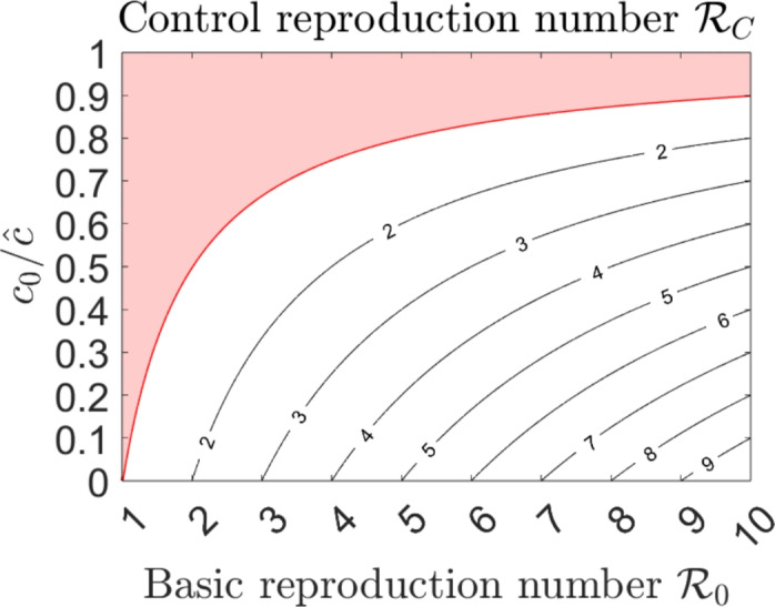
Contour plot of the control reproduction number ${\mathcal{R}}_C$ versus the basic reproduction number ${\mathcal{R}}_0$ and the ratio $c_0/\widehat{c}$. The light–red coloured region satisfies ${\mathcal{R}}_C<1$, the red line represents the curve $c_0/\widehat{c}=1-1/{\mathcal{R}}_0$

Boundary equilibria and invasion criteria

The model admits a unique virus–i–dominance equilibrium $E_i$ ($i=1,2$), a boundary equilibrium that exists if and only if ${\mathcal{R}}_{\mathit{Ci}}>1$ and represents a steady state in which only virus–i is endemic in the population. Precisely, we have:

$$\begin{array}{c}\hfill E_1=(S_1^{\ast },I_1^{\ast },0,0,R_1^{\ast },0,0,M_1^{\ast }),\end{array}$$

where:

$$\begin{array}{c}\hfill S_1^{\ast }=\frac{\mu +{\gamma }_1}{a_1(g(I_1^{\ast }))},R_1^{\ast }=\frac{{\gamma }_1}{\mu +{\rho }_1}{I}_1^{\ast },M_1^{\ast }=k_1{I}_1^{\ast },\end{array}$$

and $I_1^{\ast }$ is the unique positive root of the function

$$\begin{array}{c}\hfill \zeta (I_1)=\mu \left[1,-,\frac{\mu +{\gamma }_1}{a_1(g(I_1))}\right]+I_1\left[\frac{{\rho }_1{\gamma }_1}{\mu +{\rho }_1},-,({\gamma }_1+\mu )\right],\end{array}$$ 15

i.e., the coordinate $I_1^{\ast }$ satisfies

$$\begin{array}{c}\hfill I_1^{\ast }=\frac{(\mu +{\rho }_1)(a_1^{\ast }-\mu -{\gamma }_1)}{(\mu +{\rho }_1+{\gamma }_1)a_1^{\ast }}.\end{array}$$

Since $\zeta$ is monotonically decreasing in $I_1$ and $\zeta (0)=\mu (1-1/{\mathcal{R}}_{C1})$, there exists a unique positive root $I_1^{\ast }$ if and only if ${\mathcal{R}}_{C1}>1$.

Analogously, the virus–2–dominance equilibrium $E_2=(S_2^{\ast },0,I_2^{\ast },0,0,R_2^{\ast },0,M_2^{\ast })$ exists and is unique if and only if ${\mathcal{R}}_{C2}>1$.

In order to study the local stability of the virus–i dominance equilibrium, we compute the invasion number ${\mathcal{R}}_j^{\text{inv}}$ of virus–j at equilibrium $E_i$. It is defined as the number of secondary infections that one individual infected with virus–j will produce in a population in which virus–i is endemic, during its infectivity period (Zhang et al. 2007; Mitchell and Kribs 2019). Using the method developed by Van den Driessche and Watmough (2002), we obtain the following expression for ${\mathcal{R}}_2^{\text{inv}}$:

$$\begin{array}{c}\hfill {\mathcal{R}}_2^{\text{inv}}=\frac{{\mathrm{\Pi }}_{11}+{\mathrm{\Pi }}_{22}+\sqrt{{({\mathrm{\Pi }}_{11}-{\mathrm{\Pi }}_{22})}^2+4{\mathrm{\Pi }}_{12}{\mathrm{\Pi }}_{21}}}{2},\end{array}$$ 16

where:

$$\begin{array}{cccc}\hfill {\mathrm{\Pi }}_{11}& =\frac{[(\mu +{\rho }_1)(\mu +{\gamma }_1)+{\gamma }_1{a}_1^{\ast }{I}_1^{\ast }]a_2^{\ast }}{(\mu +{\rho }_1)[(1-q)a_4^{\ast }{I}_1^{\ast }+\mu +{\gamma }_2]a_1^{\ast }},\hfill & \hfill {\mathrm{\Pi }}_{22}& =\frac{a_4^{\ast }{I}_1^{\ast }}{\mu +{\gamma }_3},\hfill \\ \hfill {\mathrm{\Pi }}_{12}& =\frac{[(1-p)(\mu +{\rho }_1)(\mu +{\gamma }_1)+{\gamma }_1{a}_1^{\ast }{I}_1^{\ast }]a_3^{\ast }}{(\mu +{\rho }_1)(\mu +{\gamma }_3)a_1^{\ast }},\hfill & \hfill {\mathrm{\Pi }}_{21}& =\frac{a_4^{\ast }{I}_1^{\ast }}{(1-q)a_4^{\ast }{I}_1^{\ast }+\mu +{\gamma }_2},\hfill \end{array}$$

and $a_i^{\ast }=a_i(g(I_1^{\ast }))$ is the value of the i–th transmission rate ($i=1,\cdots ,4$) at the equilibrium $E_1$. Further details on the computation of ${\mathcal{R}}_2^{\text{inv}}$ are contained in Appendix B.

Analogously, the invasion number ${\mathcal{R}}_1^{\text{inv}}$ of virus–1 at the equilibrium $E_2$ has the following expression:

$$\begin{array}{c}\hfill {\mathcal{R}}_1^{\text{inv}}=\frac{{\mathrm{\Sigma }}_{11}+{\mathrm{\Sigma }}_{22}+\sqrt{{({\mathrm{\Sigma }}_{11}-{\mathrm{\Sigma }}_{22})}^2+4{\mathrm{\Sigma }}_{12}{\mathrm{\Sigma }}_{21}}}{2},\end{array}$$ 17

where:

$$\begin{array}{cccc}\hfill {\mathrm{\Sigma }}_{11}& =\frac{[(\mu +{\rho }_2)(\mu +{\gamma }_2)+{\gamma }_2{a}_2^{\ast }I_2^{\ast }]a_1^{\ast }}{(\mu +{\rho }_2)[qa_4^{\ast }I_2^{\ast }+\mu +{\gamma }_1]a_2^{\ast }},\hfill & \hfill {\mathrm{\Sigma }}_{22}& =\frac{a_4^{\ast }I_2^{\ast }}{\mu +{\gamma }_3},\hfill \\ \hfill {\mathrm{\Sigma }}_{12}& =\frac{[p(\mu +{\rho }_2)(\mu +{\gamma }_2)+{\gamma }_{2}a_2^{\ast }I_2^{\ast }]a_3^{\ast }}{(\mu +{\rho }_1)(\mu +{\gamma }_3)a_2^{\ast }},\hfill & \hfill {\mathrm{\Sigma }}_{21}& =\frac{a_4^{\ast }I_2^{\ast }}{qa_4^{\ast }I_2^{\ast }+\mu +{\gamma }_1},\hfill \end{array}$$

$a_i^{\ast }=a_i(g(I_2^{\ast }))$ is the value of the i–th transmission rate ($i=1,\cdots ,4$) at the equilibrium $E_2$ (Table 1).

Table 1.

Summary of the reproduction numbers and their interpretations. The corresponding analytical expressions are given in the indicated equations

Parameter	Symbol	Interpretation	Expression
Basic reproduction number of virus–i	${\mathcal{R}}_{0i}$	Average number of secondary infections produced by a single individual infected by virus–i, in a fully susceptible population.	(12)
Control reproduction number of virus–i	${\mathcal{R}}_{\mathit{Ci}}$	Average number of secondary infections produced by a single individual infected by virus–i, in a fully susceptible population and in the presence of control measures.	(14)
Invasion number of virus–i at virus–j dominance equilibrium	${\mathcal{R}}_i^{\text{inv}}$	Average number of secondary infections produced by a single individual infected by virus–j in a population where virus–i is endemic.	(16), (17)

The following result concerns the local stability of the virus–1 dominance equilibrium:

Proposition 4

Let us assume that ${\mathcal{R}}_{C1}>1$. If ${\mathcal{R}}_2^{\text{inv}}<1$, then the virus–1–dominance equilibrium $E_1$ is locally asymptotically stable. If ${\mathcal{R}}_2^{\text{inv}}>1$, then $E_1$ is unstable.

Proof

See Appendix B. $\square$

An analogous stability result holds for the virus–2–dominance equilibrium $E_2$.

Proposition 5

Let us assume that ${\mathcal{R}}_{C2}>1$. If ${\mathcal{R}}_1^{\text{inv}}<1$, the virus–2–dominance equilibrium $E_2$ is locally asymptotically stable. If ${\mathcal{R}}_1^{\text{inv}}>1$, then $E_2$ is unstable.

Remark 2

The relative magnitudes of the control and invasion numbers depend on whether co–infection is incorporated into the model. In particular:

(i)

If there is no co–infection (i.e., ${\widehat{a}}_4=0$), the invasion number ${\mathcal{R}}_i^{\text{inv}}$ of virus–i at the equilibrium $E_j$ assumes the following form:

$$\begin{array}{c}\hfill {\mathcal{R}}_i^{\text{inv}}=\frac{a_i(g(I_j^{\ast }))}{\mu +{\gamma }_i}\left(S_j^{\ast },+,R_j^{\ast }\right)=\frac{a_i(g(I_j^{\ast }))}{\mu +{\gamma }_i}\left[\frac{\mu +{\gamma }_j}{a_j(g(I_j^{\ast }))},+,\frac{{\gamma }_j}{\mu +{\rho }_j},I_j^{\ast }\right],\end{array}$$ 18

with $i,j=1,2,i\ne j$. Recalling that the equation (4) implies

$$\begin{array}{c}\hfill \frac{a_i(g(I_j^{\ast }))}{\mu +{\gamma }_i}=\frac{{\pi }_i(\widehat{c}-c_0)}{\mu +{\gamma }_i}\left[1,-,\frac{c_1(g(I_j^{\ast }))}{\widehat{c}-c_0}\right]={\mathcal{R}}_{\mathit{Ci}}\left[1,-,\frac{c_1(g(I_j^{\ast }))}{\widehat{c}-c_0}\right],\\ \hfill \end{array}$$ 19

it follows that ${\mathcal{R}}_i^{\text{inv}}<{\mathcal{R}}_{\mathit{Ci}}$. Therefore, if co–infection is absent, and virus–i cannot establish itself within an entirely susceptible population, it will also be unable to establish itself in a population where virus–j is endemic.

(ii)

If there is co–infection (i.e, ${\widehat{a}}_4>0$), it may be ${\mathcal{R}}_{\mathit{Ci}}<1<{\mathcal{R}}_i^{\text{inv}}$. For example, by setting: ${\widehat{a}}_1=0.3$ ${\text{d}}^{-1}$, ${\gamma }_1=1/5$ ${\text{d}}^{-1}$, ${\rho }_1=1/500$ ${\text{d}}^{-1}$, ${\widehat{a}}_2=0.24$ ${\text{d}}^{-1}$, ${\gamma }_2=1/5$ ${\text{d}}^{-1}$, ${\rho }_1=1/365$ ${\text{d}}^{-1}$, ${\widehat{a}}_3=0.7$ ${\text{d}}^{-1}$, ${\gamma }_3=1/7$ ${\text{d}}^{-1}$, ${\rho }_3=1/365$ ${\text{d}}^{-1}$, $p=0$, $q=1$ and the other parameters as in Table 2 in Section 4, we obtain that ${\mathcal{R}}_{C1}=1.199$, ${\mathcal{R}}_{C2}=0.959$, ${\mathcal{R}}_1^{\text{inv}}=1.217$ and ${\mathcal{R}}_2^{\text{inv}}=1.116$. Therefore, co–infection can facilitate the establishment of virus–i in a population where virus–j is endemic.

Table 2.

Parameter definitions of model (6), together with the values and sources used to simulate the behavioural scenario in Figure 4

Quantity	Description	Value	Source
$\mu$	Recruitment and natural death rate	$3.9·{10}^{-5}{\text{d}}^{-1}$	(Fahlena et al. 2022)
${\widehat{a}}_i$	Baseline transmission rate of virus–i ($i=1,2$)	Varies	—
${\widehat{a}}_3$	Baseline transmission rate of co–infected individuals	Varies	—
${\widehat{a}}_4$	Baseline co–infection rate	$5{\text{d}}^{-1}$	(Fahlena et al. 2022)
$a_{i,0}$	Info-independent transmission rate of virus–i ($i=1,2$)	$0.2{\widehat{a}}_i$	Assumed
$a_{3,0}$	Info-independent transmission rate of co–infected individuals	$0.2{\widehat{a}}_3$	Assumed
$a_{4,0}$	Info-independent co–infection rate	$0.2{\widehat{a}}_4$	Assumed
p	Probability that a co–infected individual transmits virus–1 to a susceptible	0.20	Assumed
q	Probability that an individual in $I_1$ gets co–infected after a contact with $I_2$	0.20	Assumed
${\gamma }_i$	Recovery rate from virus–i	$0.14{\text{d}}^{-1}$	(Fahlena et al. 2022)
${\gamma }_3$	Recovery rate from co–infection	$0.14{\text{d}}^{-1}$	(Fahlena et al. 2022)
${\rho }_i$	Loss of immunity rate towards virus–i	$0.0027{\text{d}}^{-1}$	(Fahlena et al. 2022)
${\rho }_3$	Loss of immunity rate towards co–infection	$0.0027{\text{d}}^{-1}$	(Fahlena et al. 2022)
$k_i$	Information coverage about virus–i	0.80	(Buonomo and Della Marca 2020)
$k_3$	Information coverage about co–infection	0.2	Assumed
$\delta$	Population reactivity rate	1	Assumed
$T_a$	Average information delay	3 days	(Buonomo and Della Marca 2020)

Forward bifurcation of the disease–free equilibrium

From now on, we are interested in deriving sufficient conditions for the existence and local stability of the co–endemic equilibria

$$\begin{array}{c}\hfill E_c=(S^{(c)},I_1^{(c)},I_2^{(c)},I_3^{(c)},R_1^{(c)},R_2^{(c)},R_3^{(c)},M^{(c)}),\end{array}$$

where $I_1^{(c)}$, $I_2^{(c)}$ and $I_3^{(c)}$ are strictly positive. Such equilibria represent steady states in which both diseases coexist in the population.

The following result rules out the existence of co–endemic equilibria when ${\mathcal{R}}_C<1$.

Theorem 1

Let ${\mathcal{R}}_{C2}<1$. Then the equilibrium $E_0$ of model (6) undergoes a forward bifurcation at ${\mathcal{R}}_{C1}=1$. When ${\mathcal{R}}_{C1}<1$, $E_0$ is locally asymptotically stable whereas when ${\mathcal{R}}_{C1}>1$, $E_0$ becomes unstable and a locally asymptotically stable endemic equilibrium appears.

Proof

We take ${\widehat{a}}_1$ as bifurcation parameter and use Castillo–Chavez and Song bifurcation theorem (Castillo-Chavez and Song 2004, Theorem 4.1) to show that the equilibrium $E_0$ undergoes a forward bifurcation at ${\widehat{a}}_1^{\text{thr}}=\mu +{\gamma }_1+a_{1,0}$ (the superscript “thr” indicates the threshold value). The Jacobian matrix $\tilde{J}=J(E_0,{\widehat{a}}_1^{\text{thr}})$ has the following form:

$$\begin{array}{c}\hfill \tilde{J}=\left[\begin{array}{cccccccc}-\mu & -(\mu +{\gamma }_1)& -a_2(0)& -a_3(0)& {\rho }_1& {\rho }_2& {\rho }_3& 0\\ 0& 0& 0& p{a}_3(0)& 0& 0& 0& 0\\ 0& 0& a_2(0)-\mu -{\gamma }_2& (1-p)a_3(0)& 0& 0& 0& 0\\ 0& 0& 0& -(\mu +{\gamma }_3)& 0& 0& 0& 0\\ 0& {\gamma }_1& 0& 0& -(\mu +{\rho }_1)& 0& 0& 0\\ 0& 0& {\gamma }_2& 0& 0& -(\mu +{\rho }_2)& 0& 0\\ 0& 0& 0& {\gamma }_3& 0& 0& -(\mu +{\rho }_3)& 0\\ 0& k_1/T_a& k_2/T_a& k_3/T_a& 0& 0& 0& -1/T_a\\ \end{array}\right]\end{array}$$

The right eigenvector w of $\tilde{J}$ is

$$\begin{array}{c}\hfill w={\left(-,\frac{\mu +{\rho }_1+{\gamma }_1}{{\gamma }_1},,,\frac{\mu +{\rho }_1}{{\gamma }_1},,,0,,,0,,,1,,,0,,,0,,,\frac{k_1(\mu +{\rho }_1)}{{\gamma }_1}\right)}^{\text{t}},\end{array}$$ 20

while the left eigenvector v is

$$\begin{array}{c}\hfill v=\left(0,,,\frac{{\gamma }_1}{\mu +{\rho }_1},,,0,,,\frac{p{\gamma }_1({\widehat{a}}_3-a_{3,0})}{(\mu +{\gamma }_3)(\mu +{\rho }_1)},,,0,,,0,,,0,,,0\right).\end{array}$$

Note that the component $w_j$ is nonnegative whenever ${(E_0)}_j=0$, as required in Castillo-Chavez and Song (2004, Remark 1). The direction of the bifurcation at ${\mathcal{R}}_{C1}=1$ is determined by the sign of the coefficients $\mathcal{A}$ and $\mathcal{B}$ of the normal form of the transcritical bifurcation (note that in the paper by Castillo-Chavez and Song (2004), such coefficients are denoted by a and b, respectively). We have:

$$\begin{array}{cc}\hfill \mathcal{A}& :=\sum _{k,i,j=1}^8{v}_k{w}_i{w}_j\frac{{\partial }^2{f}_k}{\partial x_i\partial x_j}(E_0,{\widehat{a}}_1^{\text{thr}})\hfill \\ \hfill & =-2\left[({\widehat{a}}_2-a_{2,0}),\frac{(\mu +{\rho }_1+{\gamma }_1)}{{\gamma }_1},+,k_1,(\mu +{\rho }_1),|a_2^{\prime }(0)|\right],\hfill \\ \hfill \mathcal{B}& :=\sum _{k,i=1}^8{v}_k{w}_i\frac{{\partial }^2{f}_k}{\partial x_i\partial {\widehat{a}}_1}(E_0,{\widehat{a}}_1^{\text{thr}})=v_2{w}_2\frac{{\partial }^2{f}_2}{\partial I_1\partial {\widehat{a}}_1}(E_0,{\widehat{a}}_1^{\text{thr}})=1.\hfill \end{array}$$

Since $\mathcal{A}<0$ and $\mathcal{B}>0$, a forward bifurcation occurs at ${\mathcal{R}}_{C1}=1$. $\square$

Remark 3

An analogous result to the one in Theorem 1 can be obtained when ${\mathcal{R}}_{C1}<1$. In this case, the equilibrium $E_0$ undergoes a transcritical forward bifurcation at ${\mathcal{R}}_{C2}=1$, with the equilibrium $E_0$ unstable and a locally asymptotically stable endemic equilibrium if ${\mathcal{R}}_{C2}>1$. Then, we can conclude that $E_0$ undergoes a transcritical forward bifurcation at ${\mathcal{R}}_C=1$.

Remark 4

Theorem 1 does not imply that the bifurcating equilibrium is necessarily $E_1$. In fact, if ${\widehat{a}}_4>0$, the bifurcating equilibrium could be the co–endemic equilibrium $E_c$ instead of $E_1$, when the invasion number ${\mathcal{R}}_2^{\text{inv}}>1$. Consequently, the theorem only rules out the existence of both endemic and co–endemic equilibria when ${\mathcal{R}}_C<1$.

Co–endemic equilibria without co–infection

In this subsection, we focus on the case without co–infection (i.e., ${\widehat{a}}_4=0$) and analyse the existence and local stability of a co–endemic equilibrium

$$\begin{array}{c}\hfill E_c=(S^{(c)},I_1^{(c)},I_2^{(c)},R_1^{(c)},R_2^{(c)},M^{(c)}),\end{array}$$

with $I_1^{(c)},I_2^{(c)}>0$. In this case, the system (6) reduces to the following subsystem:

$$\begin{array}{cc}\hfill \dot{S}(t)& =\mu -a_1(M)S{I}_1-a_2(M)S{I}_2+{\rho }_1{R}_1+{\rho }_2{R}_2-\mu S,\hfill \end{array}$$ 21a

$$\begin{array}{cc}\hfill {\dot{I}}_1(t)& =a_1(M)S{I}_1+a_1(M)R_2{I}_1-(\mu +{\gamma }_1)I_1,\hfill \end{array}$$ 21b

$$\begin{array}{cc}\hfill {\dot{I}}_2(t)& =a_2(M)S{I}_2+a_2(M)R_1{I}_2-(\mu +{\gamma }_2)I_2,\hfill \end{array}$$ 21c

$$\begin{array}{cc}\hfill {\dot{R}}_1(t)& ={\gamma }_1{I}_1-a_2(M)R_1{I}_2-(\mu +{\rho }_1)R_1,\hfill \end{array}$$ 21d

$$\begin{array}{cc}\hfill {\dot{R}}_2(t)& ={\gamma }_2{I}_2-a_1(M)R_2{I}_1-(\mu +{\rho }_2)R_2,\hfill \end{array}$$ 21e

$$\begin{array}{cc}\hfill \dot{M}(t)& =\frac{1}{T_a}(k_1{I}_1+k_2{I}_2-M),\hfill \end{array}$$ 21f

By using equations (18) and (19), we get that if $R_{C1}>R_{C2}$, then ${\mathcal{R}}_1^{\text{inv}}>1$ and the equilibrium $E_2$ is unstable. Hence, if the co–infection rate ${\widehat{a}}_4$ is set equal to zero, the equilibria $E_1$ and $E_2$ cannot be simultaneously locally asymptotically stable.

Concerning the stability of the equilibrium $E_1$, we have that it is locally stable if ${\mathcal{R}}_2^{\text{inv}}<1$ and destabilises at the bifurcation point ${\mathcal{R}}_2^{\text{inv}}=1$. In order to prove the existence of a co–endemic equilibrium when ${\mathcal{R}}_2^{\text{inv}}>1$, we perform a bifurcation analysis on the equilibrium $E_1$, choosing ${\widehat{a}}_2$ as the bifurcation parameter and denoting by ${\widehat{a}}_2^{\text{thr}}$ its value at the bifurcation point where ${\mathcal{R}}_2^{\text{inv}}=1$. Note that, if ${\widehat{a}}_2={\widehat{a}}_2^{\text{thr}}$, the value $a_2^{\text{thr}}(M_1^{\ast })$ at the equilibrium $E_1$ satisfies

$$\begin{array}{c}\hfill a_2^{\text{thr}}(M_1^{\ast })=\frac{a_1^{\ast }(\mu +{\rho }_1)(\mu +{\gamma }_2)}{(\mu +{\gamma }_1)(\mu +{\rho }_1)+{\gamma }_1{a}_1^{\ast }{I}_1^{\ast }}.\end{array}$$ 22

Theorem 2

Let ${\mathcal{R}}_{C1}>{\mathcal{R}}_{C2}>1$, so that ${\mathcal{R}}_1^{\text{inv}}>1$. Assume that one of the following two conditions holds:

• (i)
  The virus–2 infectivity rate is such that ${\gamma }_2>{\tilde{\gamma }}_2$, where:

  $$\begin{array}{c}\hfill {\tilde{\gamma }}_2:=\frac{(\mu +{\gamma }_1){(\mu +{\rho }_1)}^2}{{\gamma }_1(a_1^{\ast }-\mu -{\gamma }_1){(a_1^{\ast })}^2}\left[{(a_1^{\ast })}^2,+,k_2,|a_1^{\prime }(M_1^{\ast })|,(\mu +{\gamma }_1)\right]-\mu ,\end{array}$$ 23
• (ii)The information coverages $k_1$ and $k_2$ about virus–1 and virus–2 are equal, that is, $k_1=k_2$.

Then, the equilibrium $E_1$ undergoes a transcritical forward bifurcation at ${\mathcal{R}}_2^{\text{inv}}=1$. When ${\mathcal{R}}_2^{\text{inv}}<1$, the equilibrium $E_1$ is locally asymptotically stable; when ${\mathcal{R}}_2^{\text{inv}}>1$, $E_1$ becomes unstable and a locally stable co–endemic equilibrium $E_c$ appears.

Proof

We use the bifurcation theorem by Castillo-Chavez and Song (2004) and compute the Jacobian matrix $\tilde{J}=J(E_1)$ at the bifurcation value ${\widehat{a}}_2^{\text{thr}}$:

$$\begin{array}{c}\hfill \tilde{J}=\left[\begin{array}{cccccc}-(\mu +a_1^{\ast }{I}_1^{\ast })& -(\mu +{\gamma }_1)& -a_2^{\text{thr}}(M_1^{\ast })S_1^{\ast }& {\rho }_1& {\rho }_2& -a_1^{\prime }(M_1^{\ast })S_1^{\ast }{I}_1^{\ast }\\ a_1^{\ast }{I}_1^{\ast }& 0& 0& 0& a_1^{\ast }{I}_1^{\ast }& a_1^{\prime }(M_1^{\ast })S_1^{\ast }{I}_1^{\ast }\\ 0& 0& 0& 0& 0& 0\\ 0& {\gamma }_1& -a_2^{\text{thr}}(M_1^{\ast })R_1^{\ast }& -(\mu +{\rho }_1)& 0& 0\\ 0& 0& {\gamma }_2& 0& -(\mu +{\rho }_2+a_1^{\ast }{I}_1^{\ast })& 0\\ 0& \frac{k_1}{T_a}& \frac{k_2}{T_a}& 0& 0& -\frac{1}{T_a}\end{array}\right],\end{array}$$

where $a_1^{\prime }(M_1^{\ast })=\frac{\text{d}{a}_1}{\text{d}M}{|}_{M_1^{\ast }}$ is negative, since $a_1$ is monotonically decreasing in M.

The matrix $J(E_1)$ has one simple zero eigenvalue and all the other eigenvalues with negative real parts, so the hypothesis A1 of Castillo-Chavez and Song (2004, Theorem 4.1) is satisfied. The left eigenvector v corresponding to the zero eigenvalue is

$$\begin{array}{c}\hfill v=(0,0,1,0,0,0).\end{array}$$

Furthermore, since the right eigenvector $w=(w_1,w_2,w_3,w_4,w_5,w_6)$ has to satisfy the condition $v·w=1$, we get $w_3=1$. The other components of w have to be computed from the following linear system:

$$\begin{array}{cc}& -(\mu +a_1^{\ast }{I}_1^{\ast })w_1-(\mu +{\gamma }_1)w_2+{\rho }_1{w}_4+{\rho }_2{w}_5\hfill \\ \hfill & +|a_1^{\prime }(M_1^{\ast })|S_1^{\ast }{I}_1^{\ast }{w}_6=a_2^{\text{thr}}(M_1^{\ast })S_1^{\ast }\hfill \end{array}$$ 24a

$$\begin{array}{cc}& a_1^{\ast }{I}_1^{\ast }(w_1+w_5)+|a_1^{\prime }(M_1^{\ast })|S_1^{\ast }{I}_1^{\ast }{w}_6=0\hfill \end{array}$$ 24b

$$\begin{array}{cc}& {\gamma }_1{w}_2-(\mu +{\rho }_1)w_4=a_2^{\text{thr}}(M_1^{\ast })R_1^{\ast }\hfill \end{array}$$ 24c

$$\begin{array}{cc}& (\mu +{\rho }_2+a_1^{\ast }{I}_1^{\ast })w_5={\gamma }_2\hfill \end{array}$$ 24d

$$\begin{array}{cc}& k_1{w}_2-w_6=-k_2\hfill \end{array}$$ 24e

From equations (24d), (24e), (24e), we derive:

$$\begin{array}{c}\hfill w_4=-\frac{{\gamma }_1{a}_2^{\text{thr}}(M_1^{\ast })I_1^{\ast }}{{(\mu +{\rho }_1)}^2}+\frac{{\gamma }_1}{\mu +{\rho }_1}{w}_2,w_5=\frac{{\gamma }_2}{\mu +{\rho }_2+a_1^{\ast }{I}_1^{\ast }},w_6=k_2+k_1{w}_2,\\ \hfill \end{array}$$ 25

and using equations (24b) and (25), we can compute $w_1$ depending on $w_2$:

$$\begin{array}{c}\hfill w_1=\left[\frac{k_1|a_1^{\prime }(M_1^{\ast })|(\mu +{\gamma }_1)}{{(a_1^{\ast })}^2}\right]w_2+\left[\frac{|a_1^{\prime }(M_1^{\ast })|(\mu +{\gamma }_1)k_2}{{(a_1^{\ast })}^2},-,\frac{{\gamma }_2}{\mu +{\rho }_2+a_1^{\ast }{I}_1^{\ast }}\right].\\ \hfill \end{array}$$ 26

Furthermore, by adding equations (24a), (24b), (24c), (24d), we get:

$$\begin{array}{c}\hfill -\mu (w_1+w_2+w_4+w_5)=a_2^{\text{thr}}(M_1^{\ast })(S_1^{\ast }+R_1^{\ast })-{\gamma }_2.\end{array}$$ 27

Remembering that $a_2^{\text{thr}}$ satisfies ${\mathcal{R}}_2^{\text{inv}}=1$, we can get the following condition:

$$\begin{array}{c}\hfill {\mathcal{R}}_2^{\text{inv}}=\frac{a_2^{\text{thr}}(S_1^{\ast }+R_1^{\ast })}{\mu +{\gamma }_2}=1\Rightarrow a_2^{\text{thr}}(S_1^{\ast }+R_1^{\ast })-{\gamma }_2=\mu ,\end{array}$$

that can be substituted in (27) to get the following equation to find $w_2$:

$$\begin{array}{c}\hfill w_1+w_2+w_4+w_5=-1.\end{array}$$ 28

Note that the components $w_3$ and $w_5$ of the eigenvector w are nonnegative, as required by the hypothesis A2 of Castillo-Chavez and Song (2004, Theorem 4.1). By using (26), (25) and (28), we can compute $w_2$:

$$\begin{array}{c}\hfill w_2=\frac{{\gamma }_1{a}_2^{\text{thr}}(M_1^{\ast }){(a_1^{\ast })}^2{I}_1^{\ast }-k_2|a_1^{\prime }(M_1^{\ast })|(\mu +{\gamma }_1){(\mu +{\rho }_1)}^2-{(\mu +{\rho }_1)}^2{(a_1^{\ast })}^2}{{(\mu +{\rho }_1)}^2{(a_1^{\ast })}^2+k_1|a_1^{\prime }(M_1^{\ast })|(\mu +{\gamma }_1){(\mu +{\rho }_1)}^2+{\gamma }_1(\mu +{\rho }_1){(a_1^{\ast })}^2}.\\ \hfill \end{array}$$ 29

The direction of the bifurcation at the value ${\mathcal{R}}_2^{\text{inv}}=1$ is determined by the sign of the coefficients $\mathcal{A}$ and $\mathcal{B}$. We have:

$$\begin{array}{c}\hfill \mathcal{B}:=\sum _{k,i=1}^6{v}_k{w}_i\frac{{\partial }^2{f}_k}{\partial x_i\partial {\widehat{a}}_2}(E_1,a_2^{\text{thr}})={\partial }_{{\widehat{a}}_2}{a}_2(M_1^{\ast })(S_1^{\ast }+R_1^{\ast })>0,\end{array}$$

and:

$$\begin{array}{cc}\hfill \mathcal{A}& :=\sum _{k,i,j=1}^6{v}_k{w}_i{w}_j\frac{{\partial }^2{f}_k}{\partial x_i\partial x_j}(E_1,a_2^{\text{thr}})=a_2^{\text{thr}}(M_1^{\ast })(w_1+w_4)-|a_1^{\prime }(M_1^{\ast })|(S_1^{\ast }+R_1^{\ast })w_6\hfill \\ \hfill & =-a_2^{\text{thr}}(M_1^{\ast })\left(1,+,w_2,+,\frac{{\gamma }_2}{\mu +{\rho }_2+a_1^{\ast }{I}_1^{\ast }}\right)-|a_1^{\prime }(M_1^{\ast })|(S_1^{\ast }+R_1^{\ast })(k_2+k_1{w}_2)\hfill \\ \hfill & =-{\mathcal{C}}_1{w}_2-{\mathcal{C}}_0,\hfill \end{array}$$

where

$$\begin{array}{cc}\hfill {\mathcal{C}}_1& :=a_2^{\text{thr}}(M_1^{\ast })+k_1|a_1^{\prime }(M_1^{\ast })|(S_1^{\ast }+R_1^{\ast }),\hfill \\ \hfill {\mathcal{C}}_0& :=a_2^{\text{thr}}(M_1^{\ast })+\frac{a_2^{\text{thr}}(M_1^{\ast }){\gamma }_2}{\mu +{\rho }_2+a_1^{\ast }{I}_1^{\ast }}+k_2|a_1^{\prime }(M_1^{\ast })|(S_1^{\ast }+R_1^{\ast }).\hfill \end{array}$$

Note that both ${\mathcal{C}}_1$ and ${\mathcal{C}}_0$ are positive. If condition (i) is satisfied, then ${\gamma }_2>{\tilde{\gamma }}_2$ and $w_2>0$. This implies that $\mathcal{A}<0$ and the direction of the bifurcation is forward. If condition (ii) holds, it is easy to see from equation (29) that $w_2>-1$. Thus, we obtain:

$$\begin{array}{c}\hfill \mathcal{A}<{\mathcal{C}}_1-{\mathcal{C}}_0=-\frac{a_2^{\text{thr}}(M_1^{\ast }){\gamma }_2}{\mu +{\rho }_2+a_1^{\ast }{I}_1^{\ast }}<0,\end{array}$$

and the bifurcation is forward. $\square$

Remark 5

(i)

The analogous result can be stated for the equilibrium $E_2$ by assuming ${\mathcal{R}}_{C2}>{\mathcal{R}}_{C1}>1$, in order to have ${\mathcal{R}}_2^{\text{inv}}>1$. In this case, by taking ${\widehat{a}}_1$ as bifurcation parameter, we can give sufficient conditions for the occurrence of a forward bifurcation at ${\mathcal{R}}_1^{\text{inv}}=1$, with the equilibrium $E_2$ that is locally asymptotically stable when ${\mathcal{R}}_1^{\text{inv}}<1$ and unstable when ${\mathcal{R}}_1^{\text{inv}}>1$, with the bifurcating co–endemic equilibrium $E_c$ being locally asymptotically stable.

(ii)

Theorem 2 gives sufficient conditions guaranteeing that $\mathcal{A}<0$. However, extensive numerical simulations (not shown here) suggest that for the set of epidemiological parameters considered in this study, the coefficient $\mathcal{A}$ is negative for any values of the information–related parameters.

Effects of information–induced behavioural changes

Parameter values and initial conditions

A complete data set from field cases is not yet available for model (6). Therefore, the epidemiological parameter values are taken from Fahlena et al. (2022). In particular, as was done in Fahlena et al. (2022), we choose ${\widehat{a}}_1={\widehat{a}}_2={\widehat{a}}_3$ and denote them as $\widehat{a}$. The value of the average information delay $T_a$ is borrowed from Buonomo and Della Marca (2020), whose estimate relies on the first COVID–19 wave in Italy. The information–independent reduction rates $a_{1,0}$, $a_{2,0}$, $a_{3,0}$ and $a_{4,0}$ are guessed to be $20\%$ of the corresponding non–behavioural parameters.

Regarding the information coverages $k_1$, $k_2$ and $k_3$, we consider two different sets of values. The first set is given by $k_1=k_2=k_3=0$ and describes the situation in which the population does not reduce its social contacts, either because it does not perceive the two diseases as a health risk or because it is not informed about their prevalence. We denote this scenario as the non–behavioural scenario.

The second set of values aims to represent the behavioural scenario in which the population modifies its contact patterns due to information. We choose $k_1=k_2=0.8$ as in Buonomo and Della Marca (2020), while we assign a lower value to the co–infection information coverage, say $k_3=0.2$, since usually the official data do not provide information about the number of co–infected (World Health Organisation 2024a, b) and the perception of co–infected cases is mostly based on rumours.

Concerning the value of the population reactivity rate $\delta$, for $\delta$ varying in [0, 10], the transmission rate a(M(t)) ranges between 0.45 and 0.6 after an initial transient (see Figure 3). Therefore, taking $\delta =1$ allows to observe variations in the transmission rate a(M(t)) and, at the same time, to avoid that the transmission rate becomes negligible.

Fig. 3.

Time profiles of the transmission rate $a(t):=a_i(t)=({\widehat{a}}_i-a_{i,0})/(1+\delta M(t))$, for the population reactivity rate $\delta$ varying between 0 to 10 and baseline transmission rate ${\widehat{a}}_i=0.6$ ($i=1,2,3$)

Finally, we assume that only a small number of infected is initially present in the community, say $I_1(t_0)=0.005$ and $I_2(t_0)=0.003$, and that at the initial time $t_0$, the individuals base their behaviour only on current data, so that

$$\begin{array}{c}\hfill M(t_0)=k_1{I}_1(t_0)+k_2{I}_2(t_0)+k_3{I}_3(t_0).\end{array}$$ 30

All the parameter values of the model, together with the initial conditions, are reported in Table 2.

Effects of information–induced behavioural changes on the oscillatory dynamics

We numerically explore the solutions of model (6) for different values of the baseline transmission rate $\widehat{a}$ and compare them in the behavioural and non–behavioural scenarios introduced in the last section. The simulations, performed by using the MATLAB solver ode45, are shown in Figure 4, where the solutions in the behavioural scenario (solid lines) are overlapped to those obtained in the non–behavioural one (dotted lines).

Fig. 4.

Numerical simulations for the system (6) with different values of $\widehat{a}$ and the other parameters as in Table 2. The behavioural scenario ($k_1=k_2=0.8$, $k_3=0.2$, solid lines) is compared with the non–behavioural scenario ($k_1=k_2=k_3=0$, dotted lines). The panels on the left show the projection of the solution curve in the $I_1{I}_3$ plane and the panels on the right show the co–infected individuals $I_3(t)$ depending on time. The time intervals in the right panels are chosen for illustrative purposes

In both scenarios, a given value ${\widehat{a}}^{\ast }$ looks like a bifurcation point that marks the transition between sustained oscillations (Figure 4a) and damped oscillations towards a steady state (Figure 4c) in which the co–infection is endemic. The simulations in Figure 4 also show that the threshold value ${\widehat{a}}^{\ast }$ is lower in the behavioural scenario than in the non–behavioural one. Therefore, for some values of $\widehat{a}$ the non–behavioural scenario can exhibit sustained oscillations while the solutions of the behavioural one converge to a co–endemic equilibrium (see Figure 4b). In view of this, we can conclude that information–induced reduction of social contacts alone may produce a stabilizing effect.

Extension to vaccine–preventable respiratory viruses

Modelling vaccination and its impact on social distancing compliance

So far, we have considered the case where only non–pharmaceutical strategies were put in place to contain the epidemic. However, for many respiratory viruses, vaccines are currently available. Human behaviour may play a major role in the success of vaccination campaigns. It is recognised that vaccination behaviour may be affected by information and rumours gathered on perceived risks of getting the disease and the perceived risks of being affected by vaccine side effects (Wang et al. 2016). For example, individuals may be more prone to vaccinate when the prevalence of a virus is high and less prone to vaccinate when the prevalence decreases, as the fear of vaccine side effects begins to prevail in the benefit–cost balance (Suryawanshi and Biswas 2023; Kaushal et al. 2023). Furthermore, the implementation of vaccination policies may be combined with non–pharmaceutical containment measures (such as social distancing and wearing facial masks) as occurred during the COVID–19 pandemic. However, when these two control methods coexist, adherence to social distancing may be negatively influenced by high vaccination coverage. In fact, knowing that a high proportion of the population is vaccinated can encourage individuals to be less careful about their behaviour and to relax social distancing, relying on the efficacy of vaccines. As a consequence, such relaxation may increase viral infections (Andersson et al. 2021; Buonomo et al. 2022).

In the literature, some co–infections models that include vaccination can be found (Majeed et al. 2023; Ojo et al. 2022). However, the effects of human behavioural changes are not considered. For this reason, we extend model (6) by including vaccination. Precisely, we assume that two vaccines, say vax–1 and vax–2, are available for the disease caused by virus–1 and virus–2, respectively. Such vaccines are assumed to be no combo–like, in the sense that vax–i has no effect on the propagation of virus–j and vice-versa. A practical example is provided by the influenza and SARS-CoV-2 vaccines, which do not offer cross-protective effects (Liang et al. 2024; Del Riccio et al. 2024). The extended model is used to study two different phenomena produced by human behavioural changes: the prevalence–induced vaccination and the vaccination–induced relaxation of social distancing. Specifically, as in Buonomo et al. (2022), we assume that: (i) the choice to vaccinate against each virus is partially voluntary and depends on information about its prevalence; (ii) the choice of relaxing social distancing depends on the information about the level of vaccination compliance.

The extended model is obtained by adding three new compartments to model (6): $V_1$, $V_2$ and $V_3$, representing the individuals vaccinated only against virus–1, only against virus–2 and against both viruses, respectively. The total population, denoted by N(t), is now divided into ten disjointed compartments and

$$\begin{array}{c}\hfill N(t)=S(t)+\sum _{i=1}^3{I}_i(t)+\sum _{i=1}^3{R}_i(t)+\sum _{i=1}^3{V}_i(t).\end{array}$$

For the sake of brevity, the balance equations of the extended model are given in (48) of Appendix C, while its flow chart is shown in Figure 5.

Fig. 5.

Flowchart of model (6), extended to include vaccination. The system of balance equations for the extended model is provided in (48) (Appendix C). Recruitment into the susceptible compartment and natural death in each compartment are not shown in the diagram

The current and past values of virus–1 and virus–2 epidemics, together with current and past vaccination data, are contained in the following three information indexes:

$$\begin{array}{cc}\hfill {\mathcal{M}}_1(t)& ={\int }_0^{+\infty }{g}_1(I_1(t-\tau ),I_3(t-\tau )){\text{Erl}}_{1,1/T_1}(\tau )d\tau ,\hfill \end{array}$$ 31

$$\begin{array}{cc}\hfill {\mathcal{M}}_2(t)& ={\int }_0^{+\infty }{g}_2(I_2(t-\tau ),I_3(t-\tau )){\text{Erl}}_{1,1/T_2}(\tau )d\tau ,\hfill \end{array}$$ 32

$$\begin{array}{cc}\hfill \mathcal{V}(t)& ={\int }_0^{+\infty }h(V_1(t-\tau ),V_2(t-\tau ),V_3(t-\tau )){\text{Erl}}_{1,1/T_v}(\tau )d\tau ,\hfill \end{array}$$ 33

where $g_1$ (resp. $g_2$) is a message function that describes how knowledge of quantities $I_1$ and $I_3$ (resp. $I_2$ and $I_3$) influences the individual choice to get vaccinated against virus–1 (resp. virus–2). Analogously, the function h relates the knowledge of quantities $V_1$, $V_2$ and $V_3$ to the individual’s choice of relaxing social distance. The functions “${\text{Erl}}_1$” denote first–order Erlang distribution memory kernels and parameters $T_1$, $T_2$ and $T_v$ may be interpreted as the average time delays of the collected information about the prevalence of virus–1, virus–2 and the level of vaccination compliance, respectively.

Analogously with equation (3), we consider the following message functions:

$$\begin{array}{cc}\hfill g_1(I_1,I_3)& =k_1{I}_1+k_3{I}_3,\hfill \end{array}$$ 34

$$\begin{array}{cc}\hfill g_2(I_2,I_3)& =k_2{I}_2+k_3{I}_3,\hfill \end{array}$$ 35

$$\begin{array}{cc}\hfill h(V_1,V_2,V_3)& ={\tilde{k}}_1{V}_1+{\tilde{k}}_2{V}_2+{\tilde{k}}_3{V}_3,\hfill \end{array}$$ 36

where $k_1$, $k_2$ and $k_3$ are, respectively, the information coverage about the prevalence of virus–1, virus–2 and co–infection and ${\tilde{k}}_1$, ${\tilde{k}}_2$ and ${\tilde{k}}_3$ are the information coverages about the vaccination data.

We assume that individuals are immunised against virus–i at a vaccination rate ${\phi }_i$ and that is dependent on the information index ${\mathcal{M}}_i(t)$, given in (31) and (32). Moreover, the transmission rates $a_j$, $j=1,2,3$, and the co–infection rate $a_4$ are assumed to depend on the information index $\mathcal{V}(t)$, given in (33). The specific functional forms adopted to describe such information–dependent rates are discussed below.

i) Vaccination rates. The rate ${\phi }_i$ is given by:

$$\begin{array}{c}\hfill {\phi }_i({\mathcal{M}}_i)={\phi }_{0,i}+{\phi }_{1,i}({\mathcal{M}}_i),i=1,2.\end{array}$$ 37

The first term on the r. h. s., ${\phi }_{0,i}$, is a positive constant that represents the percentage of susceptibles who choose to get vaccinated independently of the information (for example, people strongly in favour of vaccines, health workers, fragile individuals for whom health authorities strongly recommend vaccination, etc.). The second term on the r.h.s. of (37), ${\phi }_{1,i}({\mathcal{M}}_i)$, represents the fraction of susceptibles whose vaccination choice is influenced by the information. In analogy with the function $c_1(M)$ in (4), we require that ${\phi }_{1,i}$ is a non–negative, continuous, differentiable and increasing function, ${\phi }_{1,i}(0)=0$ and $\text{sup}({\phi }_{1,i}({\mathcal{M}}_i))<{\phi }_{\text{max}}-{\phi }_{0,i}$, where ${\phi }_{\text{max}}$ is a positive upper bound. These requirements are satisfied by the following Holling type II functional:

$$\begin{array}{c}\hfill {\phi }_{1,i}({\mathcal{M}}_i)=({\phi }_{\text{max}}-{\phi }_{0,i})\frac{D_i{\mathcal{M}}_i}{1+D_i{\mathcal{M}}_i}\text{for}i=1,2,\end{array}$$

where $D_i$ is a positive constant that shapes individual reactivity to voluntary vaccination against virus–i (Buonomo et al. 2008).

ii) Transmission and co–infection rates. Motivated by the discussion in subsection 5.1 and following the notation adopted in Section 2, we set:

$$\begin{array}{c}\hfill a_j(\mathcal{V})={\pi }_j[\widehat{c}-c_0+c_1(\mathcal{V})].\end{array}$$ 38

We require that the function $c_1$ in (38) is non–negative, continuous, differentiable and increasing, $c_1(0)=0$ and $\text{sup}(c_1(\mathcal{V}))\le c_0<\widehat{c}$. These requirements are satisfied by the following Holling type II functional:

$$\begin{array}{c}\hfill c_1(\mathcal{V})=c_0\frac{\tilde{D}\mathcal{V}}{1+\tilde{D}\mathcal{V}},\end{array}$$ 39

where $\tilde{D}$ is a positive constant tuning of the reactivity of individuals to relax their social distancing and other non–pharmaceutical interventions.

Note that the difference between formulation (4) and (38) is that in the former, the rate $a_j$ decreases with the index M, while in the latter the rate $a_j$ increases with the index $\mathcal{V}$, since it causes the increase in the contact rate due to the relaxation of non–pharmaceutical measures.

Further details on the extended model, including the computation of the control reproduction number ${\mathcal{P}}_c$ and the local stability of the disease–free equilibrium $E^{\ast }$ can be found in Appendix D.

Parameter values and initial conditions

We take the values in Table 2 for all the parameters that the extended model (48) shares with model (6). The values of the vaccination–related parameters, except for ${\tilde{k}}_3$, are taken from previous theoretical investigations (Buonomo et al. 2022; Buonomo and Della Marca 2019) and are mainly guessed. Regarding the information coverages ${\tilde{k}}_1$, ${\tilde{k}}_2$ and ${\tilde{k}}_3$ we consider two different sets of values, as done in subsection 4.1. The first set is given by ${\tilde{k}}_1={\tilde{k}}_2={\tilde{k}}_3=0$ and describes the no–relaxation scenario in which the relaxation of social distancing is neglected. The second set of values represents the relaxation scenario and is given by ${\tilde{k}}_1={\tilde{k}}_2=0.95$ and ${\tilde{k}}_3=0.5{\tilde{k}}_1$. The reduced value of the information coverage ${\tilde{k}}_3$ reflects the circumstance that usually the population is not fully aware of the number of vaccinated individuals against both viruses, because such a number may be not provided by health agencies. For example, data on co-vaccinated individuals was not provided for the recent vaccination campaign against COVID–19 in the US (Centers For Disease Control and Prevention 2024b, a). Nonetheless, ${\tilde{k}}_3$ is not zero, since the population awareness depends not only on official information but also on rumours.

As for the initial conditions, reasoning as in subsection 4.1, we set:

$$\begin{array}{cc}\hfill {\mathcal{M}}_1(t_0)& =k_1{I}_1(t_0)+k_3{I}_3(t_0),\hfill \end{array}$$ 40

$$\begin{array}{cc}\hfill {\mathcal{M}}_2(t_0)& =k_2{I}_2(t_0)+k_3{I}_3(t_0),\hfill \end{array}$$ 41

$$\begin{array}{cc}\hfill \mathcal{V}(t_0)& ={\tilde{k}}_1{V}_1(t_0)+{\tilde{k}}_2{V}_2(t_0)+{\tilde{k}}_3{V}_3(t_0).\hfill \end{array}$$ 42

The guessed initial values are $I_1(t_0)=0.005$, $I_2(t_0)=0.003$, $V_1(t_0)=V_2(t_0)=0.1$.

All the vaccination–related parameters contained in the extended model, together with the values used to simulate the relaxation scenario, are reported in Table 3.

Table 3.

Definitions of the vaccination-related parameters contained in the extended model (48) and the values used to simulate the relaxation scenario. Except for the value of ${\tilde{k}}_3$, such values have been used in previous theoretical investigations (Buonomo et al. 2022; Buonomo and Della Marca 2019) and are mainly guessed

Quantity	Description	Value
${\tilde{k}}_i$	Information coverage about vax–i ($i=1,2$)	0.95
${\tilde{k}}_3$	Information coverage about individuals that received both vaccines	$0.5·{\tilde{k}}_1$
${\sigma }_i$	Factor of ineffectiveness of vax–i	0.15
${\theta }_i$	Rate of loss of immunity given by vax–i ($i=1,2$)	$0.0027{\text{d}}^{-1}$
${\theta }_3$	Rate of loss of immunity given by both vaccines	$0.0027{\text{d}}^{-1}$
${\phi }_{0,i}$	Fraction of susceptibles choosing to receive vax–i regardless of information	0.004
${\phi }_{\text{max}}$	Upper bound of the vaccination rates	0.99
$D_i$	Population reactivity to voluntarily receive vax–i ($i=1,2$)	2.5
$\tilde{D}$	Population reactivity to relax social distancing	0.25
$T_i$	Average information delay about virus–i prevalence	35 days
$T_v$	Average information delay about vaccination data	60 days

Effects of vaccination–induced relaxation of social distancing on oscillatory dynamics

As already done in subsection 4.2, we show the solutions of the extended model for different values of the baseline transmission rate $\widehat{a}$ and compare the relaxation scenario with the no–relaxation one. Figure 6 shows the comparison between the solutions obtained in the relaxation scenario (solid lines) and in the no–relaxation scenario (dotted lines), with the corresponding control reproduction numbers ${\mathcal{P}}_c$, computed using equation (50) in Appendix D. From Figure 6, we observe that the extended model admits a threshold value, say ${\mathcal{P}}_c^{\ast }$, such that when ${\mathcal{P}}_c$ crosses ${\mathcal{P}}_c^{\ast }$, the solutions pass from converging towards a co–endemic steady state (panel 6a) to exhibiting sustained oscillations over time (panel 6c).

Fig. 6.

Numerical simulations for the extended model (48) for different values of $\widehat{a}$. The other parameter values are taken as in Tables 2 and 3. The relaxation scenario ($\tilde{k}=0.95$ and ${\tilde{k}}_3=0.5\tilde{k}$, solid lines) is compared with the no–relaxation scenario ($\tilde{k}={\tilde{k}}_3=0$, dotted lines). The time intervals are chosen for illustrative purposes

However, it follows trivially from the equation (50) that the value of ${\mathcal{P}}_c$ in the no–relaxation scenario is strictly smaller than in the relaxation scenario. Consequently, for some values of $\widehat{a}$ we have ${\mathcal{P}}_c<{\mathcal{P}}_c^{\ast }$ in the no–relaxation scenario, while in the relaxation scenario we have ${\mathcal{P}}_c>{\mathcal{P}}_c^{\ast }$. This implies that the two scenarios have different long–time dynamics: sustained oscillations occur in the relaxation scenario, while damped oscillations occur in the no–relaxation one (panel 6b). This suggests that the vaccination–induced relaxation of social distancing may destabilise the model dynamics.

Impact of vaccination–related information parameters on disease prevalence, incidence and vaccinations

We investigate the impact of both the average information delay, $T_v$, and the information coverage, $\tilde{k}$ (where $\tilde{k}:={\tilde{k}}_1={\tilde{k}}_2$), on disease prevalence, incidence and vaccinations. To this aim, we consider the following relevant quantities: i) the maximum total prevalence MP(t), i.e., the highest value of total prevalence in the time frame $[t_0,t]$; ii) the total cumulative incidence CI(t), i.e., the cumulative number of new cases of virus–1 and virus–2 in the time interval $[t_0,t]$; and iii) the cumulative vaccinations CV(t), i.e., the cumulative number of vax–1 and vax–2 vaccines administered in the time interval $[t_0,t]$. They can be expressed as follows:

$$\begin{array}{cc}\hfill \text{MP}(t)& =\text{max}(I_1(\tau )+I_2(\tau )+I_3(\tau )),\tau \in [t_0,t],\hfill \\ \hfill \text{CI}(t)& ={\int }_{t_0}^t\{a_1(\mathcal{V}(\tau ))I_1(\tau )[S(\tau )+R_2(\tau )+{\sigma }_1{V}_1(\tau )+V_2(\tau )+{\sigma }_1{V}_3(\tau )]\hfill \\ \hfill & +a_2(\mathcal{V}(\tau ))I_2(\tau )[S(\tau )+R_1(\tau )+V_1(\tau )+{\sigma }_2{V}_2(\tau )+{\sigma }_3{V}_3(\tau )]\hfill \\ \hfill & +a_3(\mathcal{V}(\tau ))I_3(\tau )[S(\tau )+R_1(\tau )+R_2(\tau )+p({\sigma }_1{V}_1(\tau )+V_2(\tau )\hfill \\ \hfill & +{\sigma }_1{V}_3(\tau ))+(1-p)(V_1(\tau )+{\sigma }_2{V}_2(\tau )+{\sigma }_2{V}_3(\tau ))]\hfill \\ \hfill & +a_4(\mathcal{V}(\tau ))[I_1(\tau )I_2(\tau )+I_1(\tau )I_3(\tau )+I_2(\tau )I_3(\tau )]\}d\tau ,\hfill \\ \hfill \text{CV}(t)& ={\int }_{t_0}^t\{{\phi }_1({\mathcal{M}}_1(\tau ))[S(\tau )+V_2(\tau )]+{\phi }_2({\mathcal{M}}_2(\tau ))[S(\tau )+V_1(\tau )]\}d\tau .\hfill \end{array}$$

For illustrative purposes, we fix $\widehat{t}=120$ days and perform the contour plots of CI$(\widehat{t})$, CV$(\widehat{t})$ and MP$(\widehat{t})$ as the parameters $\tilde{k}$ and $T_v$ vary. Figure 7 shows that all the above mentioned quantities depend mainly on the information coverage $\tilde{k}$, as it can be deduced by the almost vertical contour lines. Conversely, all of them become more sensitive to variations in $T_v$ if $\tilde{k}>0.7$. Figure 7 also shows that CI$(\widehat{t})$ and MP$(\widehat{t})$ monotonically increase with $\tilde{k}$, and both of them reach their respective maximum values when $\tilde{k}=1$. This result is consistent with the fact that the transmission rates $a_1$, $a_2$ and $a_3$ as well as the co–infection rate b increase monotonically with the information index $\mathcal{V}$, and therefore they increase monotonically with $\tilde{k}={\tilde{k}}_1={\tilde{k}}_2$ in virtue of (33) and equation (36).

Fig. 7.

Contour plots of CI$(\widehat{t})$, CV$(\widehat{t})$ and MP$(\widehat{t})$, evaluated at $\widehat{t}=120$ days, versus the information coverage $\tilde{k}$ (where $\tilde{k}:={\tilde{k}}_1={\tilde{k}}_2$) and the average information delay $T_v$. The values of the parameters are reported in Tables 2 and 3 except for the baseline transmission rate, which is set $\widehat{a}=0.55{\text{d}}^{-1}$

As for the cumulative vaccinations CV$(\widehat{t})$, we find a first glance contradictory result since CV$(\widehat{t})$ decreases with $\tilde{k}$ (panel 7c) although the vaccination rates ${\phi }_1$ and ${\phi }_2$ increase monotonically with the number of infected, which in turn increase with $\tilde{k}$. However, observe that CV$(\widehat{t})$ is the result of two contrasting phenomena. From on one hand, the number of vaccinated increases as the prevalence of the two viruses increases; on the other hand, CV$(\widehat{t})$ decreases due to both the waning effect of immunisation and the high number of infected, for which vaccination is useless. The fact that the quantity CV$(\widehat{t})$ decreases with $\tilde{k}$ until its minimum value for $\tilde{k}=1$ suggests that the second phenomenon is the prevailing one.

We finally remark that, although simultaneous vaccination against different respiratory viruses is possible (Centers For Disease Control and Prevention 2024c), here we do not consider the possibility of simultaneous administration of the two vaccines. However, many numerical simulations – not reported here – show that the inclusion of simultaneous vaccination does not produce any relevant qualitative difference when compared to the solutions of the extended model.

Effects of seasonality on the spread of co–infections

Respiratory viruses can be affected by seasonal variations due to both environmental and human behavioural factors. On the one hand, low temperatures, combined with very high or very low humidity levels, may enhance the viability and transmissibility of virus droplets in the environment and negatively affect the host’s airway antiviral defences (Moriyama et al. 2020). On the other hand, the lower temperatures during the winter season in temperate climates increase indoor person-to-person contacts which could lead to enhanced virus transmission (Schweizer et al. 2007). Furthermore, travel and social gatherings during holidays favour person–to–person contacts and thus the contagion outside the usual circle of contacts. Therefore, human behaviour may play a major role in the seasonality of respiratory diseases, especially in the northern hemisphere where times of the year where humidity and temperature are the lowest coincide with winter holidays (Neumann and Kawaoka 2022).

The impact of seasonality on the transmission of respiratory diseases is often studied through epidemic models with sinusoidal transmission rates (Liu et al. 2010). However, a more realistic representation of the alternation between regular weeks and holidays is the two–state switch function adopted by Earn et al. (2000), where the transmission rate is assumed to be reduced during the summer time. Here, we assess the effect of seasonality as the result of two contrasting phenomena: on one hand, during the summer we assume that the transmission rates are reduced, which is beneficial from an epidemiological perspective; on the other hand, we consider also a reduction of the vaccination rates, which is instead detrimental.

Hence, following Buonomo et al. (2022), seasonality is incorporated in the transmission rates $a_i$ ($i=1,2,3$), the co–infection rate $a_4$ and the vaccination rates ${\phi }_j$ ($j=1,2$), by replacing the aforementioned parameters with the following ones:

$$\begin{array}{ccc}\hfill a_{i,s}(t)& ={\chi }_i(t)a_i(\mathcal{V}(t)),\hfill & \hfill i=1,\cdots ,4,\\ \hfill {\phi }_{j,s}(t)& ={\chi }_{4+j}(t){\phi }_j({\mathcal{M}}_j(t))),\hfill & \hfill j=1,2,\end{array}$$

where the subscript “s" means that the parameter under consideration incorporates seasonality and ${\chi }_l(t)$ ($l=1,\cdots ,6$) is defined to be the two–states switch representing the percentage of reduction ${ϵ}_l$ in the l–th rate occurring during the summer season:

$$\begin{array}{c}\hfill {\chi }_l(t)=\left\{\begin{array}{cc}1\hfill & \text{if}0\le t<181,\hfill \\ 1-{ϵ}_l\hfill & \text{if}181\le t\le 243,\hfill \\ 1\hfill & \text{if}243<t\le 365.\hfill \end{array}\right)\end{array}$$

Assuming that the initial time $t_0$ corresponds to January 1, the functions ${\chi }_l$ repeat periodically at intervals of length 365 days. Day $t=181$ corresponds to July 1 and day $t=243$ corresponds to September 1.

We consider two scenarios, say seasonality (resp. no–seasonality), in which seasonality is included (resp. neglected) and set ${ϵ}_l=0.25$ ($l=1,\cdots ,6$). The other parameter values are as in Tables 2 and 3. Figure 8 shows the oscillating dynamics of the seasonality scenario (red solid lines) overlapped with the solutions obtained in the no–seasonality scenario (black dotted lines). In panel 8a, where these last converge to the co–endemic equilibrium, seasonality triggers sustained oscillations, as it could be expected. In panel 8b, sustained oscillations occurs in both scenarios. However, prevalence peaks are higher in the seasonal scenario, indicating that the detrimental effects due to the reduction of the vaccination rates prevail on the beneficial ones due to the reduction of transmission. We finally point out that corners are visible at $t_{1,k}=181+365k$ and $t_{2,k}=243+365k$, $k\in \mathbb{N}$, due to the jump discontinuities in the vector field.

Fig. 8.

Numerical simulations in the seasonality (solid red lines) and no–seasonality (dotted black lines) scenarios, for different values of the baseline transmission rate $\widehat{a}$ and for ${ϵ}_l=0.25$ ($l=1,\cdots ,6$). The values of the other parameters are reported in Tables 2 and 3

Concluding remarks

The interplay between co–infections and human behaviour from a modelling perspective is attracting the attention of scholars (Hendrickx et al. 2019), although, to the best of our knowledge, it remains a topic that has been seldom explored in the literature. Here, we make new contributions by extending the qualitative analysis of the model and including behavioural changes through the use of the information index, which is a well-established method of the Behavioural Epidemiology of Infectious Diseases.

Firstly, we extend the compartmental co–infection model proposed in Fahlena et al. (2022) to a behavioural model by assuming that the contact rate depends on the information index. A qualitative analysis of the model is carried out through stability and bifurcation theory. We compute the control reproduction number ${\mathcal{R}}_C$, which depends on the percentage reduction of contact rate due to compliance with public health policies. The classical threshold condition, ${\mathcal{R}}_C=1$, holds, with a branch of stable endemic equilibria emerging from ${\mathcal{R}}_C=1$. In order to rule out the existence of both endemic and co–endemic equilibria when ${\mathcal{R}}_C<1$, we determine the direction of the bifurcation at ${\mathcal{R}}_C=1$, showing the existence of a forward transcritical bifurcation.

To analyse the local stability of the boundary endemic equilibria, we computed the invasion numbers. As for the existence and local stability of the coendemic equilibria, the determination of sufficient conditions for their existence and local stability is mathematically challenging, due to the complexity of the model. To overcome this problem, we use the center manifold theory to determine conditions that guarantee the existence of a transcritical forward bifurcation, deriving the local stability of the coendemic equilibria at least when the invasion number is close to the value 1. This result constitutes a novel contribution of this work, as to the best of our knowledge, the stability of co–endemic equilibria is usually not addressed in the literature for similar co–infection models.

In addition, through numerical simulations, we find that information–induced human behavioural changes can stabilise the system dynamics.

Secondly, the model is further extended to include vaccination. We employ three information indexes to model the interaction between the prevalence–induced vaccination and the vaccination–induced relaxation of social distancing. The main result is that the latter phenomenon may have a destabilising effect.

Finally, we assess the impact of seasonality by introducing a two–state switch function to represent the reduction of both vaccination and transmission rates during the summer season. We find that seasonality may induce the onset of sustained oscillations where the peaks of infected individuals are higher compared to the case without seasonality.

Our findings can be developed in several directions. The first open problem is to prove the existence of Hopf bifurcation for both the main model (6) and the extended model. Although the complexity of the models makes the analysis challenging, it may be possible, in principle, to use an approach similar to that used for models with comparable complexity like, e.g., in Chen et al. (2024); Zhang et al. (2020). We also plan to estimate the co–infection rates and the information–related parameters by applying the model to specific co–infection of respiratory viruses like, e.g., influenza and SARS–CoV–2, where at least partial datasets are available (Dadashi et al. 2021; Dao et al. 2021; Krumbein et al. 2023; Yan et al. 2023). Finally, a possible follow–up of this study is the introduction of actions by the public health system aimed at reducing both the health and the economic impacts of the diseases. Optimal control theory is currently one one of the most widely used ways for this purpose (Hao et al. 2024). When the control acts in a specific way on the contact rate, new phenomena like period doubling may occur (Sharbayta et al. 2022). This will be the subject of future investigations.

Appendix A. Existence of a positive invariant set

Lemma 1

Assume that all components of the initial data ${\mathbf{x}}_0$ of model (8) are strictly positive. Then, all the components of the solution $\mathbf{x}(t)$ are strictly positive for any $t>t_0$.

Proof

Let us denote by $[t_0,\eta )$ the maximal interval of existence of the solution, with $t_0<\eta \le +\infty$. Consider:

$$\begin{array}{c}\hfill t_1:=\text{sup}\{t\mid x(\tau )>0,\tau \in [t_0,t]\}.\end{array}$$ 43

Obviously, $t_1\in (t_0,\eta ]$. Equation (6a) can be rewritten as:

$$\begin{array}{c}\hfill \dot{S}(t)=b(t)-a(t)S(t),\end{array}$$ 44

where $b(t):=\mu +{\rho }_1{R}_1(t)+{\rho }_2{R}_2(t)+{\rho }_3{R}_3(t)$, and $a(t):=\mu +a_1(t)I_1(t)+a_2(t)I_2(t)+a_3(t)I_3(t)$. Multiplying both sides by $exp{\int }_{t_0}^{t}a(\tau )d\tau$, equation (44) becomes:

$$\begin{array}{c}\hfill \frac{d}{\mathit{dt}}\left\{S,(t),e^{{\int }_{t_0}^{t}a(\tau )d\tau }\right\}=b(t)e^{{\int }_{t_0}^{t}a(\tau )d\tau }.\end{array}$$

Integrating both sides from $t_0$ to $t_1$, we obtain:

$$\begin{array}{c}\hfill S(t_1)e^{{\int }_{t_0}^{1}a(\tau )d\tau }-S(t_0)={\int }_{t_0}^{1}b(s)e^{{\int }_{t_0}^{s}a(\tau )d\tau }ds,\end{array}$$

and so:

$$\begin{array}{c}\hfill S(t_1)=S(t_0)e^{-{\int }_{t_0}^{1}a(\tau )d\tau }+e^{-{\int }_{t_0}^{1}a(\tau )d\tau }{\int }_{t_0}^{1}b(s)e^{{\int }_{t_0}^{s}a(\tau )d\tau }ds>0,\end{array}$$

since b is positive on $[t_0,t_1)$. The same argument can be applied to show that $x_i(t_1)>0$ for $i=2,\cdots ,8$ and therefore $x(t_1)>0$.

Now, we show that $t_1=\eta$ and therefore $x(t)>0$, for every $t>t_0$. Suppose by contradiction that $t_1<\eta$. Since x(t) is continuous, there exists $t_2>t_1$ such that $x(t)>0$ on $[t_0,t_2]$. This leads to a contradiction, due to (43). $\square$

Proof of Proposition 1

Since the closure of a positively invariant set is still positively invariant (Amann 2011, Remark 16.3h), it follows from Lemma 1 that ${\mathbb{R}}_{+}^8$ is positively invariant.

To prove the upper bound on $x_8(t)=M(t)$, we start from equation (1). Since

$$\begin{array}{c}\hfill {\int }_0^{+\infty }Er{l}_{1,a}(\tau )d\tau =1,\end{array}$$ 45

we have that:

$$\begin{array}{cc}\hfill M(t)& ={\int }_0^{+\infty }g(I_1(t-\tau ),I_2(t-\tau ),I_3(t-\tau )){\text{Erl}}_{1,a}(\tau )d\tau \hfill \\ \hfill & \le {\int }_0^{+\infty }g(1,1,1){\text{Erl}}_{1,a}(\tau )d\tau =\sum _{i=1}^3{k}_i.\hfill \end{array}$$

The set $\mathrm{\Omega }$ is then positively invariant for the system (8). Since the solution x(t) is confined in the compact set $\mathrm{\Omega }$, it follows that $\eta =+\infty$ and the solution exists globally for $t>t_0$. $\square$

Appendix B. Invasion criteria

In order to compute the invasion number ${\mathcal{R}}_2^{\text{inv}}$ of virus–2 at the equilibrium $E_1$, we introduce:

$$\begin{array}{c}\hfill {\mathcal{F}}_2=\left[\begin{array}{c}{a}_2(M)S{I}_2+(1-p)a_3(M)S{I}_3+a_2(M)R_1{I}_2+a_3(M)R_1{I}_3\\ a_4(M)[I_1{I}_2+I_1{I}_3+I_2{I}_3]\end{array}\right]\end{array}$$

and

$$\begin{array}{c}\hfill {\mathcal{V}}_2=\left[\begin{array}{c}(1-q)a_4(M)I_1{I}_2+a_4(M)I_2{I}_3+({\gamma }_2+\mu )I_2\\ ({\gamma }_3+\mu )I_3\end{array}\right].\end{array}$$

The Jacobian matrices of ${\mathcal{F}}_2$ and ${\mathcal{V}}_2$ evaluated at the virus–1 dominance equilibrium $E_1$ give the transmission matrix

$$\begin{array}{c}\hfill F_2=\left[\begin{array}{cc}\frac{a_2^{\ast }[(\mu +{\rho }_1)(\mu +{\gamma }_1)+{\gamma }_1{a}_1^{\ast }{I}_1^{\ast }]}{(\mu +{\rho }_1)a_1^{\ast }}& \frac{a_3^{\ast }[(1-p)(\mu +{\rho }_1)(\mu +{\gamma }_1)+{\gamma }_1{a}_1^{\ast }{I}_1^{\ast }]}{(\mu +{\rho }_1)a_1^{\ast }}\\ a_4^{\ast }{I}_1^{\ast }& a_4^{\ast }{I}_1^{\ast }\end{array}\right],\end{array}$$

and the transition matrix

$$\begin{array}{c}\hfill V_2=\left[\begin{array}{cc}(1-q)a_4^{\ast }{I}_1^{\ast }+{\gamma }_2+\mu & 0\\ 0& {\gamma }_3+\mu \end{array}\right].\end{array}$$

The invasion number ${\mathcal{R}}_2^{\text{inv}}$ is the spectral radius of the following invasion matrix (Van den Driessche and Watmough 2002):

$$\begin{array}{c}\hfill \mathrm{\Pi }=F_2{V}_2^{-1}=\left[\begin{array}{ccc}{\mathrm{\Pi }}_{11}& & {\mathrm{\Pi }}_{12}\\ {\mathrm{\Pi }}_{21}& & {\mathrm{\Pi }}_{22}\end{array}\right].\end{array}$$

Proof of Proposition 4

Since ${\mathcal{R}}_{C1}>1$, the equilibrium $E_1$ exists and is unique (see Subsection 3.3). As for its local stability, conditions (A1)–(A4) of Vanden Driessche and Watmough (2002, Theorem 2) are trivially satisfied. Condition (A5) requires that if ${\mathcal{F}}_2$ is set to zero, then all eigenvalues of the Jacobian matrix $J(E_1)$ have negative real parts. In this case, four of the eigenvalues of $J(E_1)$ are ${\lambda }_1=-({\rho }_3+\mu )$, ${\lambda }_2=-({\gamma }_2+\mu )$, ${\lambda }_3=-({\gamma }_3+\mu )$, ${\lambda }_4=-(a_1^{\ast }{I}_1^{\ast }+{\rho }_2+\mu )$, while the remaining four eigenvalues can be determined from the 4x4 sub–matrix

$$\begin{array}{c}\hfill \overline{J_1}=\left[\begin{array}{cccc}-(\mu +a_1^{\ast }{I}_1^{\ast })& -(\mu +{\gamma }_1)& {\rho }_1& \frac{|a_1^{\prime }(M_1^{\ast })|}{a_1^{\ast }}(\mu +{\gamma }_1)I_1^{\ast }\\ a_1^{\ast }{I}_1^{\ast }& 0& 0& -\frac{|a_1^{\prime }(M_1^{\ast })|}{a_1^{\ast }}(\mu +{\gamma }_1)I_1^{\ast }\\ 0& {\gamma }_1& -({\rho }_1+\mu )& 0\\ 0& \frac{k_1}{T_a}& 0& -\frac{1}{T_a}\end{array}\right],\end{array}$$ 46

whose characteristic polynomial is:

$$\begin{array}{c}\hfill P(\lambda )=(\lambda +\mu )[(\lambda +q)({\lambda }^2+l_1\lambda +l_2)+(m_1\lambda +m_2)],\end{array}$$ 47

where:

$$\begin{array}{cccccc}& m_1\hfill & \hfill ={\gamma }_1{a}_1^{\ast }{I}_1^{\ast },& l_1\hfill & =\frac{1}{T_a}+a_1^{\ast }{I}_1^{\ast },& \\ \hfill & m_2\hfill & \hfill =\frac{{\gamma }_1{a}_1^{\ast }{I}_1^{\ast }}{T_a},& l_2\hfill & =\frac{a_1^{\ast }{I}_1^{\ast }}{T_a}+\frac{k_1|a_1^{\prime }(M_1^{\ast })|}{T_a{a}_1^{\ast }},& \\ \hfill & q\hfill & \hfill =\mu +{\rho }_1.\end{array}$$

Then, another eigenvalue is ${\lambda }_5=-\mu$, the others are the roots of the equation:

$$\begin{array}{c}\hfill {\lambda }^3+{\mathcal{A}}_1{\lambda }^2+{\mathcal{A}}_2\lambda +{\mathcal{A}}_3=0,\end{array}$$

with ${\mathcal{A}}_1=l_1+q$, ${\mathcal{A}}_2=l_2+m_1+q{l}_1$ and ${\mathcal{A}}_3=q{l}_2+m_2$.

Routh–Hurwitz criterion states that all roots are negative or have a negative real part if and only if: $(i){\mathcal{A}}_i>0$, $i=1,2,3$, $(ii){\mathcal{A}}_1{\mathcal{A}}_2>{\mathcal{A}}_3$. The condition (i) is clearly satisfied, while as for condition (ii) is enough to observe that:

$$\begin{array}{cc}\hfill {\mathcal{A}}_1{\mathcal{A}}_2=& (l_1+q)(l_2+m_1+q{l}_1)>\left(\frac{1}{T_a},+,q\right)(l_2+m_1)>q{l}_2+\frac{m_1}{T_a}\hfill \\ \hfill =& q{l}_2+m_2={\mathcal{A}}_3.\hfill \end{array}$$

Hence, the eigenvalues of $J(E_1)$ have negative real part and the condition (A5) of Van den Driessche and Watmough (2002, Theorem 2) is satisfied. $\square$

Appendix C. Balance equations for the extended model

The model developed in Section 5 is described by the following system of non–linear ordinary differential equations:

$$\begin{array}{cc}\hfill \dot{S}(t)& =\mu +\sum _{i=1}^3[{\rho }_i{R}_i+{\theta }_i{V}_i-a_{i}S{I}_i]-(\mu +{\phi }_1+{\phi }_2)S,\hfill \end{array}$$ 48a

$$\begin{array}{cc}\hfill \dot{I_1}(t)& =a_1(S+R_2+{\sigma }_1{V}_1+V_2+{\sigma }_1{V}_3)I_1\hfill \\ \hfill & +a_3[p(S+{\sigma }_1{V}_1+V_2+{\sigma }_1{V}_3)+R_2]I_3\hfill \\ \hfill & -a_4(q{I}_1{I}_2+I_1{I}_3)-({\gamma }_1+\mu )I_1,\hfill \end{array}$$ 48b

$$\begin{array}{cc}\hfill {\dot{I}}_2(t)& =a_2(S+R_1+V_1+{\sigma }_2{V}_2+{\sigma }_2{V}_3)I_2\hfill \\ \hfill & +a_3[(1-p)(S+V_1+{\sigma }_2{V}_2+{\sigma }_2{V}_3)+R_1]I_3\hfill \end{array}$$ 48c

$$\begin{array}{cc}& -a_4[(1-q)I_1{I}_2+I_2{I}_3]-({\gamma }_2+\mu )I_2,\hfill \end{array}$$ 48d

$$\begin{array}{cc}\hfill {\dot{I}}_3(t)& =a_4(I_1{I}_2+I_1{I}_3+I_2{I}_3)-({\gamma }_3+\mu )I_3,\hfill \end{array}$$ 48e

$$\begin{array}{cc}\hfill {\dot{R}}_1(t)& ={\gamma }_1{I}_1-(a_2{I}_2+a_3{I}_3)R_1-({\rho }_1+\mu )R_1,\hfill \end{array}$$ 48f

$$\begin{array}{cc}\hfill {\dot{R}}_2(t)& ={\gamma }_2{I}_2-(a_1{I}_1+a_3{I}_3)R_2-({\rho }_2+\mu )R_2,\hfill \end{array}$$ 48g

$$\begin{array}{cc}\hfill {\dot{R}}_3(t)& ={\gamma }_3{I}_3-({\rho }_3+\mu )R_3,\hfill \end{array}$$ 48h

$$\begin{array}{cc}\hfill {\dot{V}}_1(t)& ={\phi }_{1}S-[{\sigma }_1{a}_1{I}_1+{\sigma }_{1}p{a}_3{I}_3+a_2{I}_2+(1-p)a_3{I}_3]V_1\hfill \\ \hfill & -({\phi }_2+{\theta }_1+\mu )V_1,\hfill \end{array}$$ 48i

$$\begin{array}{cc}\hfill {\dot{V}}_2(t)& ={\phi }_{2}S-[a_1{I}_1+p{a}_3{I}_3+{\sigma }_2{a}_2{I}_2+{\sigma }_2(1-p)a_3{I}_3]V_2\hfill \\ \hfill & -({\phi }_1+{\theta }_2+\mu )V_2,\hfill \end{array}$$ 48j

$$\begin{array}{cc}\hfill {\dot{V}}_3(t)& ={\phi }_2{V}_1+{\phi }_1{V}_2-[{\sigma }_1{a}_1{I}_1+{\sigma }_{1}p{a}_3{I}_3+{\sigma }_2{a}_2{I}_2\hfill \\ \hfill & +{\sigma }_2(1-p)a_3{I}_3]V_3-(\mu +{\theta }_3)V_3,\hfill \end{array}$$ 48k

$$\begin{array}{cc}\hfill {\dot{\mathcal{M}}}_1(t)& =\frac{1}{T_1}(g_1(I_1,I_3)-{\mathcal{M}}_1),\hfill \end{array}$$ 48l

$$\begin{array}{cc}\hfill {\dot{\mathcal{M}}}_2(t)& =\frac{1}{T_2}(g_2(I_2,I_3)-{\mathcal{M}}_2),\hfill \end{array}$$ 48m

$$\begin{array}{cc}\hfill \dot{\mathcal{V}}(t)& =\frac{1}{T_v}(h(V_1,V_2,V_3)-\mathcal{V}).\hfill \end{array}$$ 48n

The rates $a_i$ ($i=1,2,3$) depend on the information index $\mathcal{V}$; the rate ${\phi }_j$ depends on the information index ${\mathcal{M}}_j$ ($j=1,2$). The explicit dependence is here omitted for the sake of clarity. The system is equipped with the following initial conditions:

$$\begin{array}{c}\hfill \begin{array}{c}\hfill S(t_0)>0,I_i(t_0)\ge 0,R_i(t_0)\ge 0,V_i(t_0)\ge 0,i=1,2,3,\\ \hfill {\mathcal{M}}_1(t_0)\ge 0,{\mathcal{M}}_2(t_0)\ge 0,\mathcal{V}(t_0)\ge 0.\end{array}\end{array}$$ 49

We also set $N(t_0)=1$, so that $N(t)=1$ for $t>t_0$.

Appendix D. Basic analysis for the extended model

Using the same arguments of Proposition 1, we can show that the solutions of the extended model exist, are unique in the interval $[t_0,\infty )$ and are contained in the following positively invariant set $\mathcal{D}$:

$$\begin{array}{c}\hfill \mathcal{D}=\left\{\mathbf{x},\in ,{\mathbb{R}}_{+}^{13},,:,,\sum _{i=1}^{10},x_i,=,1,,,,{\mathcal{M}}_1,\le ,k_1,+,k_3,,,,{\mathcal{M}}_2,\le ,k_2,+,k_3,,,,\mathcal{V},\le ,\sum _{i=1}^3,{\tilde{k}}_i\right\}.\end{array}$$

The extended model admits the disease–free equilibrium:

$$\begin{array}{c}\hfill E^{\ast }=(S^{\ast },0,0,0,0,0,0,V_1^{\ast },V_2^{\ast },V_3^{\ast },0,0,{\mathcal{V}}^{\ast }),\end{array}$$

where:

$$\begin{array}{cccc}\hfill S^{\ast }& =\frac{[{\eta }_1-(1+{\rho }_2){\phi }_{0,1}][{\eta }_2-(1+{\rho }_1){\phi }_{0,2}]}{{\eta }_1{\eta }_2-{\phi }_{0,1}{\phi }_{0,2}(1+{\rho }_1)(1+{\rho }_2)},\hfill & \hfill V_3^{\ast }& ={\rho }_2{V}_1^{\ast }+{\rho }_1{V}_2^{\ast },\hfill \\ \hfill V_i^{\ast }& ={\phi }_{0,i}\frac{{\eta }_j-(1+{\rho }_i){\phi }_{0,j}}{{\eta }_1{\eta }_2-{\phi }_{0,1}{\phi }_{0,2}(1+{\rho }_1)(1+{\rho }_2)},\hfill & \hfill {\mathcal{V}}^{\ast }& ={\tilde{k}}_1{V}_1^{\ast }+{\tilde{k}}_2{V}_2^{\ast }+{\tilde{k}}_3{V}_3^{\ast },\hfill \end{array}$$

and

$$\begin{array}{c}\hfill {\rho }_i=\frac{{\phi }_{0,i}}{\mu +{\theta }_3},{\eta }_i={\phi }_{0,1}+{\phi }_{0,2}+{\theta }_i+\mu +{\rho }_j{\phi }_{0,i},\end{array}$$

for $i=1,2$ and $j\ne i$.

The basic reproduction number ${\mathcal{P}}_0$ of the extended model coincides with the one obtained for model (6). As for the control reproduction number ${\mathcal{P}}_c$, we follow the notations adopted by Diekmann et al. (1990) and Van den Driessche and Watmough (2002) and introduce:

$$\begin{array}{c}\hfill \mathcal{F}={\displaystyle \left[\begin{array}{c}{a}_1(\mathcal{V})(S+R_2+{\sigma }_1{V}_1+V_2+{\sigma }_1{V}_3)I_1+a_3(\mathcal{V})\\ [p(S+{\sigma }_1{V}_1+V_2+{\sigma }_1{V}_3)+R_2]I_3\\ a_2(\mathcal{V})(S+R_1+V_1+{\sigma }_2{V}_2+{\sigma }_2{V}_3)I_2+a_3(\mathcal{V})\\ [(1-p)(S+V_1+{\sigma }_1{V}_2+{\sigma }_2{V}_3)+R_1]I_3\\ a_4(\mathcal{V})(I_1{I}_2+I_1{I}_3+I_2{I}_3)\end{array}\right]}\end{array}$$

and

$$\begin{array}{c}\hfill \mathcal{V}=\left[\begin{array}{c}{a}_4(\mathcal{V})(q{I}_1{I}_2+I_1{I}_3)+({\gamma }_1+\mu )I_1\\ a_4(\mathcal{V})[(1-q)I_1{I}_2+I_2{I}_3]+({\gamma }_2+\mu )I_2\\ ({\gamma }_3+\mu )I_3\end{array}\right].\end{array}$$

The transmission matrix F is given by:

$$\begin{array}{c}\hfill F=\left[\begin{array}{ccc}{a}_1({\mathcal{V}}^{\ast }){\omega }_1& 0& p{a}_3({\mathcal{V}}^{\ast }){\omega }_1\\ 0& a_2(\mathcal{V}){\omega }_2& (1-p)a_3(\mathcal{V}){\omega }_2\\ 0& 0& 0\end{array}\right],\end{array}$$

where ${\omega }_i=1-(1-{\sigma }_i)(V_i^{\ast }+V_3^{\ast })$, $i=1,2$.

The transition matrix V is given by:

$$\begin{array}{c}\hfill V=\left[\begin{array}{ccc}\mu +{\gamma }_1& 0& 0\\ 0& \mu +{\gamma }_2& 0\\ 0& 0& \mu +{\gamma }_3\end{array}\right].\end{array}$$

The control reproduction number ${\mathcal{P}}_c$ is the spectral radius of the next generation matrix $K=F{V}^{-1}$. We have:

$$\begin{array}{c}\hfill K=\left[\begin{array}{ccc}\frac{a_1({\mathcal{V}}^{\ast }){\omega }_1}{\mu +{\gamma }_1}& 0& p{a}_3({\mathcal{V}}^{\ast }){\omega }_1\\ 0& \frac{a_2({\mathcal{V}}^{\ast }){\omega }_2}{\mu +{\gamma }_2}& (1-p)a_3({\mathcal{V}}^{\ast }){\omega }_2\\ 0& 0& 0\end{array}\right].\end{array}$$

By introducing ${{\mathcal{P}}_c}_i:=K_{\mathit{ii}}$ ($i=1,2$) and using equation (38) and equation (39), we get:

$$\begin{array}{cc}\hfill {{\mathcal{P}}_c}_i& =\left(1,-,\frac{c_0}{\widehat{c}(1+\tilde{D}{\mathcal{V}}^{\ast })}\right){\omega }_i{{\mathcal{R}}_0}_i.\hfill \end{array}$$ 50

Finally, we obtain the control reproduction number ${\mathcal{P}}_c$:

$$\begin{array}{c}\hfill {\mathcal{P}}_c=max\{{{\mathcal{P}}_c}_1,{{\mathcal{P}}_c}_2\}.\end{array}$$

From Van den Driessche and Watmough (2002, Theorem 2), we can derive the classical threshold condition:

Proposition 6

The disease-free equilibrium $E^{\ast }$ of the extended model is locally asymptotically stable if ${\mathcal{P}}_c<1$ and unstable if ${\mathcal{P}}_c>1$.

Funding

Open access funding provided by Università degli Studi di Napoli Federico II within the CRUI-CARE Agreement.

Data availability statement

Data sharing not applicable to this article as no datasets were generated or analysed during the current study.

Declaration

Conflict of interest

The author states that there is no conflict of interest.

References

- Amann H (2011) Ordinary differential equations: an introduction to nonlinear analysis, vol 13. Walter de Gruyter, Germany [Google Scholar]
- Andersson O, Campos-Mercade P, Meier AN, Wengström E (2021) Anticipation of COVID-19 vaccines reduces willingness to socially distance. J Health Econ 80:102530 [DOI] [PMC free article] [PubMed] [Google Scholar]
- Bai L, Zhao Y, Dong J, Liang S, Guo M, Liu X, Wang X, Huang Z, Sun X, Zhang Z et al (2021) Coinfection of influenza a virus enhances SARS-CoV-2 infectivity. Cell Res 31(4):395–403 [DOI] [PMC free article] [PubMed] [Google Scholar]
- Bergstrom CT, Hanage WP (2024) Human behavior and disease dynamics. Proc Natl Acad Sci 121(1):e2317211120 [DOI] [PMC free article] [PubMed] [Google Scholar]
- Bhowmick S, Sokolov IM, Lentz HH (2023) Decoding the double trouble: a mathematical modelling of coinfection dynamics of SARS-CoV-2 and Influenza-like illness. Biosystems 224:104827 [DOI] [PMC free article] [PubMed] [Google Scholar]
- Bolze A, Basler T, White S, Dei Rossi A, Wyman D, Dai H, Roychoudhury P, Greninger AL, Hayashibara K, Beatty M et al (2022) Evidence for SARS-CoV-2 delta and omicron coinfections and recombination. Med 3(12):848–859 [DOI] [PMC free article] [PubMed] [Google Scholar]
- Buonomo B, Della Marca R (2019) Oscillations and hysteresis in an epidemic model with information-dependent imperfect vaccination. Math Comput Simul 162:97–114 [Google Scholar]
- Buonomo B, Della Marca R (2020) Effects of information-induced behavioural changes during the COVID-19 lockdowns: the case of Italy. Royal Soc Open Sci 7(10):201635 [Google Scholar]
- Buonomo B, Della Marca R, d’Onofrio A, Groppi M (2022) A behavioural modelling approach to assess the impact of COVID-19 vaccine hesitancy. J Theor Biol 534:110973 [DOI] [PMC free article] [PubMed] [Google Scholar]
- Buonomo B, Della Marca R, Sharbayta SS (2022) A behavioral change model to assess vaccination-induced relaxation of social distancing during an epidemic. J Biol Syst 30(01):1–25 [Google Scholar]
- Buonomo B, d’Onofrio A, Lacitignola D (2008) Global stability of an SIR epidemic model with information-dependent vaccination. Math Biosci 216(1):9–16 [DOI] [PubMed] [Google Scholar]
- Castillo-Chavez C, Song B (2004) Dynamical models of tuberculosis and their applications. Math Biosci Eng 1(2):361–404 [DOI] [PubMed] [Google Scholar]
- Centers For Disease Control and Prevention. Influenza vaccination coverage and intent for vaccination, adults 18 years and older, United States, (2024). https://www.cdc.gov/fluvaxview/dashboard/adult-coverage.html?CDC_AAref_Val=https://www.cdc.gov/flu/fluvaxview/dashboard/vaccination-adult-coverage.html. Accessed on March 2025
- Centers For Disease Control and Prevention. Weekly COVID–19 vaccination dashboard, (2024). https://www.cdc.gov/covidvaxview/weekly-dashboard/index.html. Accessed on March 2025
- Centers For Disease Control and Prevention. What to know about getting flu, COVID–19, and RSV vaccines at the same time, (2024). https://www.cdc.gov/ncird/whats-new/getting-vaccines-at-same-time.html. Accessed on March 2025
- Chen W, Zhang L, Wang N, Teng Z (2024) Bifurcation analysis and chaos for a double-strains HIV coinfection model with intracellular delays, saturated incidence and logistic growth. Math Comput Simul 223:617–641 [Google Scholar]
- Collinson S, Khan K, Heffernan JM (2015) The effects of media reports on disease spread and important public health measurements. PLoS ONE 10(11):e0141423 [DOI] [PMC free article] [PubMed] [Google Scholar]
- Cox FEG (2001) Concomitant infections, parasites and immune responses. Parasitology 122(S1):S23–S38 [DOI] [PubMed] [Google Scholar]
- Dadashi M, Khaleghnejad S, Abedi Elkhichi P, Goudarzi M, Goudarzi H, Taghavi A, Vaezjalali M, Hajikhani B (2021) COVID-19 and influenza co-infection: a systematic review and meta-analysis. Front Med 8:681469 [Google Scholar]
- Dao TL, Colson P, Million M, Gautret P et al (2021) Co-infection of SARS-CoV-2 and influenza viruses: a systematic review and meta-analysis. J Clinical Virology Plus 1(3):100036 [DOI] [PMC free article] [PubMed] [Google Scholar]
- Del Riccio M, Caini S, Bonaccorsi G, Lorini C, Paget J, van der Velden K, Cosma C (2024) Influenza vaccination and covid-19 infection risk and disease severity: a systematic review and multilevel meta-analysis of prospective studies. Am J Infect Control 52(9):1091–1098 [DOI] [PubMed] [Google Scholar]
- Devi P, Khan A, Chattopadhyay P, Mehta P, Sahni S, Sharma S, Pandey R (2021) Co-infections as modulators of disease outcome: minor players or major players? Front Microbiol 12:664386 [DOI] [PMC free article] [PubMed] [Google Scholar]
- Diekmann O, Heesterbeek J, Roberts MG (2010) The construction of next-generation matrices for compartmental epidemic models. J R Soc Interface 7(47):873–885 [DOI] [PMC free article] [PubMed] [Google Scholar]
- Diekmann O, Heesterbeek JAP, Metz JAJ (1990) On the definition and the computation of the basic reproduction ratio R0 in models for infectious-diseases in heterogeneous populations. J Math Biol 28:365–382 [DOI] [PubMed] [Google Scholar]
- Dror AA, Eisenbach N, Taiber S, Morozov NG, Mizrachi M, Zigron A, Srouji S, Sela E (2020) Vaccine hesitancy: the next challenge in the fight against COVID-19. Eur J Epidemiol 35(8):775–779 [DOI] [PMC free article] [PubMed] [Google Scholar]
- d’Onofrio A, Manfredi P (2009) Information-related changes in contact patterns may trigger oscillations in the endemic prevalence of infectious diseases. J Theor Biol 256(3):473–478 [DOI] [PubMed] [Google Scholar]
- d’Onofrio A, Manfredi P, Salinelli E (2007) Vaccinating behaviour, information, and the dynamics of SIR vaccine-preventable diseases. Theor Popul Biol 71(3):301–317 [DOI] [PubMed] [Google Scholar]
- Earn DJ, Rohani P, Bolker BM, Grenfell BT (2000) A simple model for complex dynamical transitions in epidemics. Science 287(5453):667–670 [DOI] [PubMed] [Google Scholar]
- Fahlena H, Kusdiantara R, Nuraini N, Soewono E (2022) Dynamical analysis of two-pathogen coinfection in Influenza and other respiratory diseases. Chaos Solitons & Fractals 155:111727 [Google Scholar]
- Gumel AB, Ruan S, Day T, Watmough J, Brauer F, Driessche P, Gabrielson D, Bowman C, Alexander ME, Ardal S et al (2004) Modelling strategies for controlling SARS outbreaks. Proc R Soc Lond Ser B Biol Sci 271(1554):2223–2232 [Google Scholar]
- Hamelin FM, Allen LJ, Bokil VA, Gross LJ, Hilker FM, Jeger MJ, Manore CA, Power AG, Rúa MA, Cunniffe NJ (2019) Coinfections by noninteracting pathogens are not independent and require new tests of interaction. PLoS Biol 17(12):e3000551 [DOI] [PMC free article] [PubMed] [Google Scholar]
- Hao W, Zhang J, Jin Z (2024) Dynamic analysis and optimal control of HIV/AIDS model with ideological transfer. Math Comput Simul 226:578–605 [Google Scholar]
- Hendrickx DM, Abrams S, Hens N (2019) The impact of behavioural interventions on co-infection dynamics: an exploration of the effects of home isolation. J Theor Biol 476:5–18 [DOI] [PMC free article] [PubMed] [Google Scholar]
- Kaushal A, Mandal A, Khanna D, Acharjee A (2023) Analysis of the opinions of individuals on the COVID-19 vaccination on social media. Digital Health 9:20552076231186250 [DOI] [PMC free article] [PubMed] [Google Scholar]
- Khataee H, Scheuring I, Czirok A, Neufeld Z (2021) Effects of social distancing on the spreading of COVID-19 inferred from mobile phone data. Sci Rep 11(1):1661 [DOI] [PMC free article] [PubMed] [Google Scholar]
- Kinoshita T, Watanabe K, Sakurai Y, Nishi K, Yoshikawa R, Yasuda J (2021) Coinfection of SARS-CoV-2 and Influenza virus causes more severe and prolonged pneumonia in hamsters. Sci Rep 11(1):21259 [DOI] [PMC free article] [PubMed] [Google Scholar]
- Krumbein H, Kümmel LS, Fragkou PC, Thölken C, Hünerbein BL, Reiter R, Papathanasiou KA, Renz H, Skevaki C (2023) Respiratory viral co-infections in patients with COVID-19 and associated outcomes: a systematic review and meta-analysis. Rev Med Virol 33(1):e2365 [DOI] [PMC free article] [PubMed] [Google Scholar]
- Lewnard JA, Lo NC (2020) Scientific and ethical basis for social-distancing interventions against COVID-19. Lancet Infect Dis 20(6):631–633 [DOI] [PMC free article] [PubMed] [Google Scholar]
- Liang J, Wang Y, Lin Z, He W, Sun J, Li Q, Zhang M, Chang Z, Guo Y, Zeng W et al (2024) Influenza and covid-19 co-infection and vaccine effectiveness against severe cases: a mathematical modeling study. Front Cell Infect Microbiol 14:1347710 [DOI] [PMC free article] [PubMed] [Google Scholar]
- Liu W, Li Z-D, Tang F, Wei M-T, Tong Y-G, Zhang L, Xin Z-T, Ma M-J, Zhang X-A, Liu L-J et al (2010) Mixed infections of pandemic H1N1 and seasonal H3N2 viruses in 1 outbreak. Clin Infect Dis 50(10):1359–1365 [DOI] [PubMed] [Google Scholar]
- Majeed B, David JF, Bragazzi NL, McCarthy Z, Grunnill MD, Heffernan J, Wu J, Woldegerima WA (2023) Mitigating co-circulation of seasonal influenza and COVID-19 pandemic in the presence of vaccination: a mathematical modeling approach. Front Public Health 10:1086849 [DOI] [PMC free article] [PubMed] [Google Scholar]
- Manfredi P, d’Onofrio A (2013) Modeling the interplay between human behavior and the spread of infectious diseases. Springer Science & Business Media, Germany [Google Scholar]
- Masters NB, Shih S-F, Bukoff A, Akel KB, Kobayashi LC, Miller AL, Harapan H, Lu Y, Wagner AL (2020) Social distancing in response to the novel coronavirus (COVID-19) in the united states. PLoS ONE 15(9):e0239025 [DOI] [PMC free article] [PubMed] [Google Scholar]
- Mitchell C, Kribs C (2019) Invasion reproductive numbers for periodic epidemic models. Infect Dis Model 4:124–141 [DOI] [PMC free article] [PubMed] [Google Scholar]
- Moriyama M, Hugentobler WJ, Iwasaki A (2020) Seasonality of respiratory viral infections. Annu Rev Virol 7(1):83–101 [DOI] [PubMed] [Google Scholar]
- Neumann G, Kawaoka Y (2022) Seasonality of influenza and other respiratory viruses. EMBO Mol Med 14(4):e15352 [DOI] [PMC free article] [PubMed] [Google Scholar]
- Ojo MM, Benson TO, Peter OJ, Goufo EFD (2022) Nonlinear optimal control strategies for a mathematical model of COVID-19 and influenza co-infection. XXPhys A 607:128173 [Google Scholar]
- Pérez-Losada M, Arenas M, Galán JC, Palero F, González-Candelas F (2015) Recombination in viruses: mechanisms, methods of study, and evolutionary consequences. Infect Genet Evol 30:296–307 [DOI] [PMC free article] [PubMed] [Google Scholar]
- Pinky L, Dobrovolny HM (2022) Epidemiological consequences of viral interference: a mathematical modeling study of two interacting viruses. Front Microbiol 13:830423 [DOI] [PMC free article] [PubMed] [Google Scholar]
- Piret J, Boivin G (2022) Viral interference between respiratory viruses. Emerg Infect Dis 28(2):273 [DOI] [PMC free article] [PubMed] [Google Scholar]
- Schweizer C, Edwards RD, Bayer-Oglesby L, Gauderman WJ, Ilacqua V, Juhani Jantunen M, Lai HK, Nieuwenhuijsen M, Künzli N (2007) Indoor time-microenvironment-activity patterns in seven regions of europe. J Expo Sci Environ Epidemiol 17(2):170–181 [DOI] [PubMed] [Google Scholar]
- Sharbayta SS, Buonomo B, d’Onofrio A, Abdi T (2022) ‘period doubling’ induced by optimal control in a behavioural SIR epidemic model. Chaos Solitons & Fractals 161:112347 [Google Scholar]
- Suryawanshi YN, Biswas DA (2023) Herd immunity to fight against COVID-19: a narrative review. Cureus 15(1):e33575 [DOI] [PMC free article] [PubMed] [Google Scholar]
- Troiano G, Nardi A (2021) Vaccine hesitancy in the era of COVID-19. Public Health 194:245–251 [DOI] [PMC free article] [PubMed] [Google Scholar]
- Van den Driessche P, Watmough J (2002) Reproduction numbers and sub-threshold endemic equilibria for compartmental models of disease transmission. Math Biosci 180(1–2):29–48 [DOI] [PubMed] [Google Scholar]
- Wang Z, Bauch CT, Bhattacharyya S, d’Onofrio A, Manfredi P, Perc M, Perra N, Salathé M, Zhao D (2016) Statistical physics of vaccination. Phys Rep 664:1–113 [Google Scholar]
- West R, Michie S, Rubin GJ, Amlôt R (2020) Applying principles of behaviour change to reduce SARS-CoV-2 transmission. Nat Hum Behav 4(5):451–459 [DOI] [PubMed] [Google Scholar]
- World Health Organisation. COVID–19 epidemiological updates and monthly operational updates, (2024). https://www.who.int/emergencies/diseases/novel-coronavirus-2019/situation-reports. Accessed on March 2025
- World Health Organisation. Global influenza programme, surveillance outputs, (2024). https://www.who.int/teams/global-influenza-programme/surveillance-and-monitoring/influenza-surveillance-outputs. Accessed on March 2025
- Wu A, Mihaylova VT, Landry ML, Foxman EF (2020) Interference between rhinovirus and influenza a virus: clinical data analysis and experimental infection study. The Lancet Microbe 1(6):e254–e262 [DOI] [PMC free article] [PubMed] [Google Scholar]
- Yan X, Li K, Lei Z, Luo J, Wang Q, Wei S (2023) Prevalence and associated outcomes of co-infection between SARS-CoV-2 and influenza: a systematic review and meta-analysis. Int J Infect Dis 136:29–36 [DOI] [PubMed] [Google Scholar]
- Zhang P, Sandland GJ, Feng Z, Xu D, Minchella DJ (2007) Evolutionary implications for interactions between multiple strains of host and parasite. J Theor Biol 248(2):225–240 [DOI] [PubMed] [Google Scholar]
- Zhang X-S, Cao K-F et al (2014) The impact of coinfections and their simultaneous transmission on antigenic diversity and epidemic cycling of infectious diseases. Biomed Res Int 2014(1):375862 [DOI] [PMC free article] [PubMed] [Google Scholar]
- Zhang X-S, Angelis D, White PJ, Charlett A, Pebody RG, McCauley J (2013) Cocirculation of Influenza a virus strains and emergence of pandemic via reassortment: the role of cross-immunity. Epidemics 5(1):20–33 [DOI] [PubMed] [Google Scholar]
- Zhang Z, Kundu S, Tripathi JP, Bugalia S (2020) Stability and hopf bifurcation analysis of an SVEIR epidemic model with vaccination and multiple time delays. Chaos Solitons & Fractals 131:109483 [Google Scholar]
- Zhou Y, Xu R, Hu D, Yue Y, Li Q, Xia J (2020) Effects of human mobility restrictions on the spread of COVID-19 in shenzhen, china: a modelling study using mobile phone data. The Lancet Digital Health 2(8):e417–e424 [DOI] [PMC free article] [PubMed] [Google Scholar]
Associated Data
This section collects any data citations, data availability statements, or supplementary materials included in this article.