

Abstract
We demonstrate the feasibility of computing realistic spatial proton distributions for proteins in solution from experimental NMR nuclear Overhauser effect data only and with minimal assignments. The method, CLOUDS, relies on precise and abundant interproton distance restraints calculated via a relaxation matrix analysis of sets of experimental nuclear Overhauser effect spectroscopy crosspeaks. The MIDGE protocol was adapted for this purpose. A gas of unassigned, unconnected H atoms is condensed into a structured proton distribution (cloud) via a molecular dynamics simulated-annealing scheme in which the internuclear distances and van der Waals repulsive terms are the only active restraints. Proton densities are generated by combining a large number of such clouds, each computed from a different trajectory. After filtering by reference to the cloud closest to the mean, a minimal dispersion proton density (foc) is identified. The latter affords a quasi-continuous hydrogen-only probability distribution that conveys immediate information on the protein surface topology (grooves, protrusions, potential binding site cavities, etc.), directly related to the molecular structure. Feasibility of the method was tested on NMR data measured on two globular protein domains of low regular secondary structure content, the col 2 domain of human matrix metalloproteinase-2 and the kringle 2 domain of human plasminogen, of 60 and 83 amino acid residues, respectively.
Keywords: relaxation matrix|NOE-only structure|protein hydrogen-only structure
Despite its inherent built-in approximations, the relaxation matrix (R) analysis of NMR 1H Overhauser data such as that obtained from multidimensional nuclear Overhauser effect spectroscopy (NOESY) experiments affords the most objective procedure for deriving a self-consistent set of precise interatomic distances that can be used as constraints to verify or refine molecular structures (1–3). Such applications imply a starting structure that serves to generate an initial distance matrix D, which in turn provides a basis for the back-calculation of a complete, hybrid NOESY matrix. The latter then yields improved distances, which lead to a better structure. However, as exemplified by the MIDGE protocol (4), under the assumption of isotropic motion the values estimated for the diagonal terms of R may be improved iteratively from the better resolved off-diagonal terms. The derived interproton distances can be shown to be rather insensitive to initial hypotheses regarding the three-dimensional molecular structure. Thus, it is suggested that MIDGE-derived distances can be taken advantage of to generate spatial proton distributions compatible with the experimental NOESY data even in the absence of prior assignments. This would afford an alternative to the standard approach to NMR biomolecular structure determination that proceeds via assigned NOESY restraints (5).
Attempts aimed at deriving spatial proton distributions from nuclear Overhauser effect (NOE) data exclusively (6, 7) or supplemented with extra NMR information (8) have been reported. These studies were based on synthetic NOESY intensities or distances computed from x-ray crystallographic coordinates. Although the results variously suggested the feasibility for computation of three-dimensional structure from unassigned distance restraints (8), they also implied access to excellent quality stereo-resolved data (7). Therefore, a consensus has evolved that one of the major obstacles of such “direct” NMR approach to protein-structure elucidation is an inherent requirement for both large number and high accuracy of distance restraints, bordering on the qualities of “perfect,” i.e., synthetic, data.
As we demonstrate here, direct computation of a meaningful medium-resolution molecular hydrogen atom map is feasible even when starting from experimental interproton distances such as those derived via a self-consistent MIDGE-type analysis of unassigned, but otherwise unambiguous, NOEs. To generate the spatially organized proton distribution or “cloud” (6), a proton gas is subjected to the distance restraints. By annealing many times, each dynamic trajectory launched from a different random point in phase space, a “family of clouds” (“foc”) is generated that reflects the statistical uncertainty of the derived spatial location of each hydrogen atom in the molecule.
The results obtained on NOESY data measured from two globular protein domains, the col 2 of human matrix metalloproteinase-2 and the kringle 2 of human plasminogen, show that the proton densities obtained via CLOUDS are consistent with the structures generated by using standard NMR protocols (9, 10). Furthermore, as expanded in the accompanying paper (11), the foc density serves as a template to compute the molecular structure.
Methods
CLOUDS proceeds as follows. N unassigned proton NMR chemical shifts are extracted from standard multidimensional experiments and listed. NOESY-based interproton distances are obtained via MIDGE (4). A gas of randomly distributed H atoms then is subjected to a force field consisting solely of NMR-derived distance restraints and a repulsive van der Waals term. The pseudoenergy is subsequently minimized through a molecular dynamics/simulated annealing procedure, ANNEAL, which creates a cloud, a hydrogen-only molecular structure devoid of covalent linkages. A foc, selected via FILTER, yields a three-dimensional proton density, in real space.
NMR Spectroscopy and Computational Procedures.
Two globular protein domains, on which excellent unambiguously identified homonuclear 1H NOE listings are available, were chosen to test the CLOUDS protocol: (i) the second type II module from human matrix metalloproteinase 2 (col 2, 60 residues; ref. 9) and (ii) the kringle 2 from human plasminogen (kringle 2, 83 residues; ref. 10). Two-dimensional NOESY crosspeak volumes used for the calculations were measured from spectra recorded at 500 and 600 MHz with NOESY mixing times (τmix) of 60, 120, and 200 ms for col 2 and 60, 90, and 250 ms for kringle 2 complexed with the ligand trans-(aminomethyl)cyclohexane carboxylic acid in 1H2O (10% 2H2O) (9, 10). All calculations were carried out on Dell Precision PCs with dual 300- and 450-MHz Intel Pentium II processors running WINDOWS NT. The programs were written in FORTRAN and compiled with DIGITAL VISUAL FORTRAN 6.0. Molecular dynamics calculations were carried out by using CNS 1.0 (12), and molecular graphics were implemented through MOLMOL 2.5.1 (13).
Calculation of the Distance Matrix (MIDGE).
The NOESY matrix, A (14), may be expressed as
 |
1 |
where the τmix is the experimental thermal equilibration period, R is the relaxation matrix, and Ao = A (0). R encodes for the rate constants of dipole–dipole self-relaxation Rii = ρi and crossrelaxation Rij = σij. In the standard model (15, 16), the σij values are given by
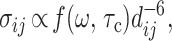 |
2 |
where dij is the interproton distance, and f(ω,τc) is a linear combination of the spectral density functions Jn = Jn(ω,τc) for the n quanta relaxation pathway (n = 0, 1, 2) that depend on the spin Larmor frequency ω and, assuming isotropic molecular tumbling, a single rotational correlation time, τc. Eq. 1 is the starting point for deriving R, and Eq. 2 is the basis for obtaining interatomic distances.
An improved MIDGE (version 2.0) was used for obtaining an optimized R from experimental NOESY (Fig. 1). Measured peak volumes were corrected for the spectral excitation profile (17), symmetrized, and normalized to the number of protons at τmix = 0 to produce the input A matrix. Groups of magnetically equivalent spins such as methyl protons were identified from line widths and intensities of their diagonal peaks. Amide HN resonances were also recognizable from, e.g., 1H/2H exchange experiments. Initially, volumes of unobserved or unresolved A peaks were set to 0 (crosspeaks) or 1 (diagonal peaks). Subsequently, A1, the generated input matrix, was converted to R1, the initial R matrix (interconversions between A and R matrix elements take into account the number of magnetically equivalent spins according to the formalism outlined in ref. 18.). The diagonal elements of R1, ρi, then were improved by combining, after suitable scaling,
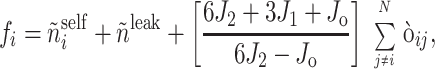 |
3 |
with the previous estimates of ρi (Fig.
1). The updated ρi elements were inserted back
into R1 to obtain
R2. For methyl protons, Eq. 3
includes corrections
ρ for
self-relaxation in groups of equivalent spins (19) or, in the case of
HN atoms, for crossrelaxation with the bound
14N nuclei (20). The
ρleak term accounts for extraneous
magnetization exchange with the environment.
for
self-relaxation in groups of equivalent spins (19) or, in the case of
HN atoms, for crossrelaxation with the bound
14N nuclei (20). The
ρleak term accounts for extraneous
magnetization exchange with the environment.
Figure 1.

MIDGE flowchart. A, the experimental (input) NOESY matrix; Ad, the diagonal submatrix of A; I, the unit matrix. A1, R1, A2, R2, Δ1, Δ2, Λ1, and Λ2 are defined in the flowchart. X1 and X2 represent the matrices of A1 and R2 eigenvectors, respectively, α is an adjustable convergence parameter, and D is the interproton distance matrix (output). The correction fi, as well as γn and ΔRn are defined in the text (Eqs. 3–5). Matrices are in bold or enclosed in square brackets.
Eq. 3 was implemented iteratively, yielding estimates for the intensities of the unresolved diagonal and unobserved, low-amplitude, off-diagonal NOESY peaks. An indicator for convergence in two consecutive iterations, n − 1 and n, was:
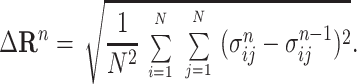 |
4 |
An index of error was defined as
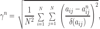 |
5 |
where the aij and
δ(aij) are A-matrix elements
and their experimental uncertainties, respectively, and each
a is the nth iteration computed value of
aij. The process was repeated until
convergence, thus generating a symmetric A matrix that is
self-consistent in terms of values for its diagonal and off-diagonal
elements. To minimize γn (Eq. 5),
τc and ρleak were
treated as adjustable parameters, optimized on a suitable grid, and
α, a convergence rate factor, was set to 0.5. An average distance
matrix D
{dij}, as well
as the corresponding rms deviation (rmsd) values, were computed from
NOESY experiments at various τmix settings.
However, only interproton distance values corresponding to nonzero
elements of the experimental A were retained for further
calculations.
is the nth iteration computed value of
aij. The process was repeated until
convergence, thus generating a symmetric A matrix that is
self-consistent in terms of values for its diagonal and off-diagonal
elements. To minimize γn (Eq. 5),
τc and ρleak were
treated as adjustable parameters, optimized on a suitable grid, and
α, a convergence rate factor, was set to 0.5. An average distance
matrix D
{dij}, as well
as the corresponding rms deviation (rmsd) values, were computed from
NOESY experiments at various τmix settings.
However, only interproton distance values corresponding to nonzero
elements of the experimental A were retained for further
calculations.
Generation of Cloud Proton Distribution (ANNEAL).
Protons, initially distributed randomly, were subjected to a pseudopotential consisting of a van der Waals repulsive term combined with a soft square-well attractive potential based on the dij values. The pseudoenergy was optimized via molecular dynamics by cooling the proton gas from 2,000 to 10 K for 100 ps. To bias the algorithm toward deriving proton distributions compatible with the absence of specific NOEs, an additional annealing from 500 to 10 K was implemented with anti-distance constraints (ADCs; refs. 21 and 22) enforced for 50 ps on those HN/HN (col 2 and kringle 2) and HN/Hα (kringle 2) proton pairs that did not yield detectable NOESY crosspeaks. The resulting cloud coordinates were stored for further analysis.
Selection of Foc Proton Density (FILTER).
Totals of ≈1,000 hydrogen-only clouds were computed for col 2 and kringle 2 and optimally superimposed according to ref. 23. For each cloud taken as a pivot, the average of pairwise interproton distance rmsds over the set, 〈rmsd〉, was calculated for the backbone atoms. The average and the standard deviation of 〈rmsd〉 were calculated for the complete set of pivot clouds. Those yielding 〈rmsd〉 > 2σc, where σc is the standard deviation from the average, were rejected. The cloud with the lowest 〈rmsd〉 was selected as reference to align all accepted clouds, and the resulting superimposition, foc, was stored for further use. Thus, the foc may be considered to represent an effective proton density based solely on the NOE distance restraints.
Results and Discussion
Interproton Distances.
MIDGE 2.0 is stable with respect to the trial set of adjustable τc and ρleak parameters. Its convergence also proves to be independent of the initial choices of diagonal elements of A as long as their initial values are set >1. The procedure converged to diagonal element volumes that, for peaks that were well resolved, agreed within 9% with the measured values (γ = 2.9 and 3.7 for col 2 and kringle 2, respectively). Furthermore, the scheme avoided negative eigenvalues for A, which lead to singularities downstream in the algorithm (Fig. 1).
On average, the col 2 and kringle 2 experimental NOESY data (Table 1) provided 3.2 and 3.5 restraints per atom, respectively. The internuclear distances computed at three τmix settings differ by ≈5% for col 2 and ≈8% for kringle 2 (averaged rmsds). From numerical experiments on model-based synthetic data sets (not shown), an average of <20% rmsd and >3 NOEs per hydrogen atom were found to be required for CLOUDS to yield a reliable proton distribution. When CLOUDS distance restraints were estimated from τmix = 60 ms NOESY experiments via the initial-rate approximation, the quality of proton distributions was poor, leading us to recur to longer τmix data, for which a relaxation matrix analysis is to be preferred.
Table 1.
CLOUDS input data
Number of 1H spins input to MIDGE.
Number of restraints generated via MIDGE and input to ANNEAL.
Number of unambiguous ADCs input to ANNEAL.
Clouds and foc.
The calculation of a single cloud required 16 minutes for col 2 and 19 minutes for kringle 2. A total of 1,200 simulated annealing/molecular dynamic runs for col 2 produced clouds with restraints violations <0.5 Å. For kringle 2, of 1,100 computed clouds 5 had a single violation >0.5 Å and were discarded. The low frequencies of violations reflect the length of the annealing protocol as well as the fact that the input H atoms are unconstrained by chemical bonds such that distance restraints are satisfied more readily. Although as gauged by the pseudo energy cost function ADCs are transiently perturbative, they were accommodated by the end of the simulations, indicating that they are neither redundant nor diverting with respect to the NOE constraints. Furthermore, by alleviating the effects of experimental NOESY sparseness, ADCs significantly improved convergence to the target atomic distributions.
The obtained clouds were split evenly into mirror image-related subsets, and ≈50% had to be reflected. Otherwise, the >1,000 computed col 2 and kringle 2 clouds showed high pairwise similarity within each protein type. The calculation of the set of average backbone H atom pairwise rmsds, 〈rmsd〉, by reference to the entire set of cloud pivots took ≈40 minutes. The plots of the combined 〈rmsd〉 versus the chosen pivot cloud are shown in Fig. 2. Reflecting scarcity of local restraints, abnormally high 〈rmsd〉 values resulted from regions of local inverted geometry within the pivot cloud. Relative to kringle 2, the higher incidence of odd structures in the case of col 2 is likely to be a consequence of the smaller number of input ADCs rather than the topology of the particular protein fold. From inspection of Fig. 2, it is apparent that the 〈rmsd〉 score affords a good criterion for rejecting aberrant structures, as the extent of variability for this index is large relative to its standard deviation.
Figure 2.

Deviations of the cloud ensemble by reference to individual clouds: col 2 (A) and kringle 2 (B). Each cloud is selected as “pivot” for cloud alignment. The dispersion of backbone HN and Hα coordinates relative to the mean is gauged by the average rmsd, 〈rmsd〉, plotted against pivot number. For each cloud, HN atoms were constrained by both NOEs and HN/HN ADCs; HN/Hα ADCs were incorporated for kringle 2 (see Table 1).
Selected single clouds for each col 2 and kringle 2 are shown in Fig. 3. Interestingly, although the all-H clouds provide rather coarse images of the atomic distribution (Fig. 3 A and C), in each case the underlying molecular architecture is conveyed clearly by the array of amide HN atoms only, from which it is possible to trace rather well defined segments of the polypeptide backbone (Fig. 3 B and D).
Figure 3.

Individual clouds for col 2 (A and B) and kringle 2 (C and D). All H atoms are included in A and C; HN atoms only are shown in B and D. The illustrated clouds are those closest to the average (minimal 〈rmsd〉; see Fig. 2).
Totals of 955 col 2 clouds and 1,048 kringle 2 clouds remained after FILTER and were superimposed to generate the molecular focs. Fig. 4 shows stereo views of the backbone (HN and Hα) atomic focs of col 2 and kringle 2. Overall, individual H atoms are well defined, and the shapes and main topological features of each domain are readily recognizable.
Figure 4.

Stereo views of molecular focs (backbone H atoms only). (A) col 2; (B) kringle 2. HN and Hα atoms are shown in blue and green, respectively. The illustrated focs are all-cloud overlaps by reference to the cloud closest to the average (see Fig. 3).
The entries in Table 2 indicate that col 2 and kringle 2 focs are of comparable quality in terms of both precision (foc rmsds) and accuracy (atomic distances to reported NMR structures; refs. 9 and 10). Coincidentally, the values of precision and accuracy turn out to be similar to each other. Not unexpectedly, both correlate with the number of NOE distance constraints at each proton site (Fig. 5), being generally higher at the molecular core than at the outer regions (Fig. 6). An example of good foc geometry is provided by the H-atom configuration of the Trp-40 indole ring in col 2 (Fig. 7). For these six atoms, the angles between the vectors normal to the planes, as defined by all possible combinations of three centers of filtered atomic distributions, are 15 ± 6°, which points to a remarkable degree of planarity. For kringle 2, the three Trp rings are less well defined, exhibiting angular indices that vary from 31 ± 16° (Trp-72) or 33 ± 22° (Trp-25) to 52 ± 22° (Trp-62). However, as is apparent from inspection of Fig. 4, the global picture is quite satisfactory in that the previously reported NMR backbone structures (9, 10) nicely fit the computed hydrogen density. Thus, notwithstanding some poor local, mostly side chain, geometries, the complete foc provides a reliable description of the overall molecular fold.
Table 2.
Statistics of cloud ensembles within focs and within reported sets of NMR structures (9, 10), and comparison between mean structures
| col
2
|
kringle 2
|
|||||
|---|---|---|---|---|---|---|
| HN | Hα | Hother | HN | Hα | Hother | |
| foc structures, Å* | 1.4 ± 0.5 | 1.8 ± 0.8 | 2.4 ± 1.1 | 1.1 ± 0.4 | 1.5 ± 0.6 | 2.1 ± 1.1 |
| Reported structures, Å* | 0.8 ± 0.4 | 0.8 ± 0.5 | 1.4 ± 0.9 | 0.5 ± 0.3 | 0.6 ± 0.3 | 1.2 ± 0.8 |
| foc to reported structures, ņ | 1.0 ± 0.5 | 1.3 ± 0.6 | 2.2 ± 1.0 | 1.5 ± 0.8 | 2.0 ± 1.0 | 2.7 ± 1.4 |
rmsd values relative to the mean.
rmsd values mean to mean.
Figure 5.

Precision (A) and accuracy (B) of atomic locations for all foc H atoms versus the number of NOE restraints for each H atom. (A) Atomic distance rmsds relative to the foc average. (B) Individual atom distances from their foc means to their means in reported NMR structures (9, 10). The histograms combine col 2 and kringle 2 data, one point per each of 766 atoms.
Figure 6.

Precision of focs along the backbone. (A) col 2. (B) kringle 2. Rmsd values are relative to foc averages. ●, backbone hydrogens (averaged HN and Hα); ○, side chain hydrogens (averaged).
Figure 7.

Col 2 Trp-40: aromatic ring foc. (A) Front view. (B) Edge side view with Hɛ1 in front. The nitrogen-bound Hδ1 is shown in blue. The atomic focs are depicted after filtering, by which 25% of the points farthest removed from each updated atomic center of mass were successively discarded.
Summary.
The self-consistency of MIDGE (Fig. 1) alleviates the effects of sparseness in the experimental NOESY matrix. The absence of an a priori structural model, a main advantage of the protocol, allows for the derivation of unbiased interproton distances. By reference to the previously reported NMR structures (Table 2 and Fig. 4), our study shows that the CLOUDS protocol yields proton densities that are consistent with the atomic positions encoded by those molecular models. Such an agreement validates the CLOUDS protocol as a basis to generate molecular structures and provides a promising starting point for developing novel automated methods to obtain protein structures via NMR.
As formulated in this paper, CLOUDS represents a minimalistic approach. However, by supplementing the input NOE data with additional restraints extracted from experiments that report on J-connected fragments, its convergence as well as overall quality of the derived proton densities can be improved further without compromising CLOUDS' main appeal, namely, the avoidance of spectral assignment. Moreover, the relaxation matrix treatment can, in principle, be improved by including local dynamics (24).
To generate the molecular structure, each hydrogen in the protein has to be nested optimally in its corresponding foc atomic density, a problem similar to fitting the protein fold to the x-ray crystallographic electron density map. In the accompanying paper (11) we propose a protocol designed to achieve this goal.
Acknowledgments
This research was sponsored by the U.S. Public Health Service, National Institutes of Health Grant HL-29409.
Abbreviations
- NOESY
nuclear Overhauser effect spectroscopy
- R
relaxation matrix
- D
interproton distances matrix
- NOE
nuclear Overhauser effect
- A
NOESY matrix
- rmsd
rms deviation
- ADC
anti-distance constraint
References
- 1.Boelens R, Koning T M G, Van Der Marel G A, Van Boom J H, Kaptein R. J Magn Reson. 1989;82:290–308. [Google Scholar]
- 2.Borgias B A, James T L. J Magn Reson. 1990;87:475–487. [Google Scholar]
- 3.Zhang Q, Chen J Y, Gozansky E K, Zhu F, Jackson P L, Gorenstein D G. J Magn Reson B. 1995;106:164–169. doi: 10.1006/jmrb.1995.1027. [DOI] [PubMed] [Google Scholar]
- 4.Madrid M, Llinás E, Llinás M. J Magn Reson. 1991;93:329–346. [Google Scholar]
- 5.Wüthrich K. NMR of Proteins and Nucleic Acids. New York: Wiley; 1986. pp. 117–199. [Google Scholar]
- 6.Malliavin T E, Rouh A, Delsuc M A, Lallemand J-Y. C R Acad Sci. 1992;315:653–659. [Google Scholar]
- 7.Oshiro C M, Kuntz I D. Biopolymers. 1993;33:107–105. doi: 10.1002/bip.360330110. [DOI] [PubMed] [Google Scholar]
- 8.Kraulis P J. J Mol Biol. 1994;243:696–718. doi: 10.1016/0022-2836(94)90042-6. [DOI] [PubMed] [Google Scholar]
- 9.Briknarová K, Grishaev A, Banyai L, Tordai H, Patthy L, Llinás M. Structure (London) 1999;7:1235–1245. doi: 10.1016/s0969-2126(00)80057-x. [DOI] [PubMed] [Google Scholar]
- 10.Marti D N, Schaller J, Llinás M. Biochemistry. 1999;38:15741–15755. doi: 10.1021/bi9917378. [DOI] [PubMed] [Google Scholar]
- 11.Grishaev A, Llinás M. Proc Natl Acad Sci USA. 2002;99:6713–6718. doi: 10.1073/pnas.042114399. [DOI] [PMC free article] [PubMed] [Google Scholar]
- 12.Brünger A T, Adams P D, Clore G M, DeLano W L, Gros P, Grosse-Kunstleve R W, Jiang J S, Kuszewski J, Nilges M, Pannu N S, et al. Acta Crystallogr D. 1998;54:905–921. doi: 10.1107/s0907444998003254. [DOI] [PubMed] [Google Scholar]
- 13.Koradi R, Billeter M, Wüthrich K. J Mol Graphics. 1996;14:51–55. doi: 10.1016/0263-7855(96)00009-4. [DOI] [PubMed] [Google Scholar]
- 14.Macura S, Ernst R R. Mol Phys. 1980;41:95–117. [Google Scholar]
- 15.Solomon I. Phys Rev. 1955;99:559–565. [Google Scholar]
- 16.Neuhaus D, Williamson M. The Nuclear Overhauser Effect in Structural and Conformational Analysis. New York: VCH; 1989. pp. 23–61. [Google Scholar]
- 17.Piotto M, Saudek V, Sklenar V. J Biomol NMR. 1992;2:661–665. doi: 10.1007/BF02192855. [DOI] [PubMed] [Google Scholar]
- 18.Olejniczak E T. J Magn Reson. 1989;81:392–394. [Google Scholar]
- 19.Yip P F, Case D A. In: Computational Aspects of the Study of Biological Macromolecules by Nuclear Magnetic Resonance Spectroscopy. Hoch J C, editor. New York: Plenum; 1991. pp. 317–330. [Google Scholar]
- 20.Llinás M, Klein M P, Wüthrich K. Biophys J. 1978;24:849–861. doi: 10.1016/S0006-3495(78)85424-1. [DOI] [PMC free article] [PubMed] [Google Scholar]
- 21.De Vlieg J, Boelens R, Scheek R M, Kaptein R, van Gunsteren W F. Isr J Chem. 1986;27:181–188. [Google Scholar]
- 22.Bruschweiler R, Blackledge M, Ernst R R. J Biomol NMR. 1991;1:3–11. doi: 10.1007/BF01874565. [DOI] [PubMed] [Google Scholar]
- 23.Kabsch W. Acta Crystallogr A. 1976;32:922–923. [Google Scholar]
- 24.Dellwo M J, Wand J. J Biomol NMR. 1993;3:205–214. doi: 10.1007/BF00178262. [DOI] [PubMed] [Google Scholar]