A survey on deep learning for polygenic risk scores

Abstract

Polygenic risk scores (PRS) combine the effects of multiple genetic variants to predict an individual’s genetic predisposition to a disease. PRS typically rely on linear models, which assume that all genetic variants act independently. They often fall short in predictive accuracy and are not able to explain the genetic variability of a trait to the full extent. There is growing interest in applying deep learning neural networks to model PRS given their ability to model non-linear relationships and strong performance in other domains. We conducted a survey of the literature to investigate how neural networks model PRS. We categorize deep learning-based approaches by their underlying architecture, highlighting their modeling assumptions, likely strengths and potential weaknesses of the architectures. Several categories of neural network architectures exhibited promising signs for the improvement of PRS’ predictive power, namely sequence-based architectures, graph neural networks and those that incorporated biological knowledge. Additionally, the use of latent representations in autoencoders has improved predictive performance across diverse ancestries. However, a lack of existing model benchmarks on consistent datasets and phenotypes makes it challenging to understand the extent to which different architectures improve performance. Interpretability of deep learning-based PRS is also challenging with great care required when inferring causation. To address these challenges, we suggest the establishment and adherence to reporting standards and benchmarks to aid the development of deep learning-based PRS to find quantifiable trends in neural network architectures.

Introduction

Polygenic risk scores (PRS) are powerful tools for predicting complex diseases. PRS estimate genetic predisposition to a disease based on the cumulative effects of numerous genetic variants, each with a small effect on risk. Using PRS, populations can be stratified into risk categories, enabling preventative measures to be targeted to those at highest risk. PRS are being explored in a range of conditions including, but not limited to, heart disease, diabetes, auto-immune conditions, and, cancer, considering quantitative as well as qualitative (categorical) traits [1–4]. Recently, a PRS has also been used to validate causal associations between sarcopenia and the risk or progression of Parkinson’s disease [5]. While showing promise, the existing methodologies for constructing PRS have several weaknesses as they are not able to explain the entirety of the genetic phenotypic variation of a trait, leaving some missing heritability.

PRS are based on a linear combination of SNPs that have shown a statistically significant association with the target disease in previous genome-wide association studies (GWAS). GWAS typically use common SNPs that have a population prevalence of 1% or more, and associations are typically tested by a regression model that yields a P-value for every SNP [6]. This approach overlooks complex gene–gene interactions, interactions between SNPs, non-additive effects, and the effects of rare variants. More advanced methodologies take into account genetic architectures, patterns of linkage, or genomic annotations but are still fundamentally based on linear models [7]. In addition to the problem of missing heritability, PRS struggle to generalize across populations [8, 9].

With data available in large biobanks and with machine learning being successfully applied in other fields, there is interest in applying deep learning to the development of PRS. The motivation lies in machine learning algorithms being able to describe non-linear relationships. The architecture of a neural network determines the flow of information and allows the integration of information about the data. This can result in substantial improvements in performance compared with a linear model.

This review focuses on the emerging applications of deep learning for the construction of PRS. Based on a systematic evaluation of the literature, we categorize the observed approaches based on their neural network architectures, from feedforward models to graph neural networks. For each category of architecture, we provide an overview of why that style of architecture was developed and then explore the PRS implementations that have used the architecture, highlighting their assumptions, strengths and weaknesses, both in method and evaluation. Finally, we discuss key challenges in the development of deep learning based PRS, including the complexities of genomic data, the difficulty in model interpretation, and systematic issues with evaluation across the literature. By systematically categorizing existing approaches and understanding their limitations, we aim to inform future development towards more accurate and robust methodologies for genomic prediction.

Literature search strategy

We searched academic databases, including Google Scholar and PubMed, as well as the University of Melbourne’s library catalog and digital repositories. In the search, we combined the keywords “PRS,” “polygenic risk score,” “neural network,” “deep learning,” “SNP,” “SNV,” and “polygenic score.” Additionally, the references of all manuscripts found in the databases were also investigated. In the end, we included 25 studies in this review that specifically construct a PRS using a deep neural network.

PRS construction and evaluation

Linear PRS

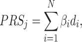
To create a linear PRS, only SNPs with the smallest P-values for association with the trait of interest are chosen. Typically, SNPs are selected at P-values to control for multiple testing, a threshold originally derived based on the number of independent common variants in populations of European ancestries [10]. The regression coefficients are estimated for each SNP and multiplied by the number of effect alleles (dosage), which can take the values 0 for no effect allele, 1 for a single effect allele, and 2 for two effect alleles. The sum over all these products yields the PRS (1) [11]. This model is considered the classical PRS model and should serve as the baseline model for comparison with more complex PRS models, it is defined as:

(1)

where , and the number of SNPs.

The goal of a PRS is to discriminate individuals at increased risk for a trait from individuals at lower risk. If successful, cases and controls from a population should be able to be separated according to Fig. 1.

Figure 1.

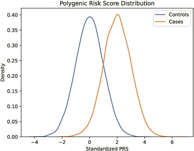
Conceptual histogram of a normalized polygenic risk score in a population, where the score is able to segregate controls and cases fairly well.

Extensions to this approach include: clumping and thresholding; stacked clumping and thresholding [12]; LDpred [13]; LDpred2 [14]; penalized regression (lassosum) [15]; and Bayesian regression (SBayesR [16] and PRS-CS [17]). In clumping and thresholding, the PRS is optimized by testing several P-value thresholds, stacked clumping and thresholding improves on that by stacking multiple of those clumping and thresholding PRS together. LDpred estimates effect sizes through an external reference panel that yields information on linkage disequilibrium (LD) together with a genetic architecture prior. LDpred2 improves LDpred by making it more robust through the use of a larger LD window size, better handling of numerical errors and a larger hyperparamater search-space [14]. Lassosum penalizes the effects of SNPs by filtering out less significant SNPs, yielding a sparser model. Lastly, Bayesian-based PRS yield credible intervals for effect sizes.

For prediction of binary traits, one of the most used metrics of a model’s discriminatory performance is the area under the receiver operating characteristic curve (AUC):

(2)

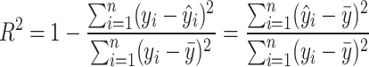
where TPR and FPR are the true and false positive rates, respectively [18]. Metrics that do not measure the ability of a model to distinguish between affected and unaffected individuals are and Nagelkerke . Both measure the proportion of variance explained by the model, which is the model’s goodness-of-fit.

(3)

where are observed values, are predicted values, is the mean of the observed values, and is the sample size.

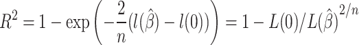(4)

, and are log likelihoods [19]. A log likelihood measures how well a model fits the observed data.

Deep learning architectures in PRS

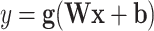
A neural network (Fig. 2a) is a non-linear regression model. The fundamental units in a neural network (neurons or perceptrons) are organized into layers: the input layer receives data; hidden layers process information through weighted connections and an output layer produces predictions. Each neuron is connected to neurons in adjacent layers, with the connections carrying weights that adjust as the network learns from the data. By stacking hidden layers between the input and output layers, a hierarchical structure is formed, allowing patterns to be learned at different levels of abstraction, from simple relationships in the early layers to complex interactions in the deeper layers. As such, neural networks can capture increasingly complex features and interactions in the data, a characteristic that makes them particularly suited for high-dimensional datasets. A key challenge is determining the correct network architecture (the configuration of the hidden layers and their connections). Different architectures embed different information and assumptions about the prediction task. A convolutional neural network (CNN) builds upon the observation that nearby pixels in an image are related and spatial patterns should be location invariant. The CNN in Fig. 2b, achieves this through a filter that slides over the image. The diagram also shows a simple multi-layer perceptron (MLP) with fully connected layers (Fig. 2a), a long short-term memory network (LSTM) (Fig. 2c) a transformer handling sequential information (Fig. 2d), a graph neural network (GNN) modeling the relationships between SNPs in a biological network (Fig. 2e), and an autoencoder performing dimensionality reduction (Fig. 2f).

Figure 2.

The surveyed deep learning-based approaches for PRS prediction can be grouped by their underlying architecture, as all architectures impose some assumptions on the SNP input data and process the SNPs differently, modeling interactions between SNPs. The six different neural network architectures found with respect to PRS are (a) MLPs, (b) CNNs, (c) LSTMs, (d) transformers, (e) GNN, and (f) autoencoders.

Neural network fundamentals

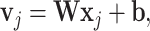
A single perceptron processes data by taking in a matrix or vector as input and yielding a weighted sum of the input and an offset as the output after applying an activation function, which in most cases introduces a non-linearity [20]:

(5)

where is a vector, 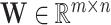is the weight matrix of a hidden layer with being the width of the layer, is a bias term, and the function is an activation function. Commonly used activation functions include:

(6)

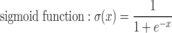(7)

(8)

(9)

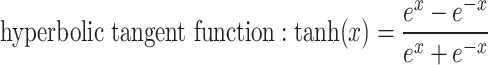
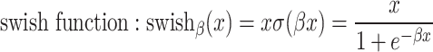
The swish function was empirically shown to work better than the most commonly used ReLU [21].

A single-layer neural network can approximate any continuous function [22]. Using the ReLU activation function [23], a hidden layer with units can approximate any dimensional Lebesgue integrable function, which should cover all functions in the scope of this work [24]. For example, to approximate a 1D function, we would require a hidden layer with at least five neurons.

Fully connected neural network

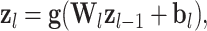
From a single perceptron, a more complex model can be created by connecting and stacking multiple perceptrons in a network, which leads to a popular neural network architecture, the fully connected neural network (FCNN), also known as a multi-layer perceptron (MLP). In an FCNN, each layer takes in data in the form of a vector, applies a weighting matrix and a bias term, and then applies a non-linearity in the form of an activation function. Subsequent layers (hidden layers) take the output of this operation as the input vector (6). The neural network is fully connected when every entry in the output layer serves as input for the next layer [25]. As information only flows in one direction from the input towards the output layer, it is a feedforward neural network. Each layer is formally described as

(10)

where is a vector, is a vector is the weight matrix of a hidden layer with being the width of the layer, is a bias term, and the function is an activation function such as ReLU (6) or swish (9).

The final output layer reduces the dimension of the feature vector to the number of classes in a classification problem, yielding a probability per class, or in the case of regression, an approximation of the target variable.

One approach for PRS development with an FCNN is to predict the risk from the SNP dosage as an input vector, a input vector consisting of entries 0, 1, and 2. The network then discriminates individuals at risk by predicting their phenotype. The likelihood of a class in the final output layer is in most cases used as the PRS.

In the case of PRS prediction, an FCNN can be used to model linear or non-linear interactions between SNPs, such as epistasis [26], which is a phenomenon where the presence of a variant of an allele suppresses the effect of another allele [27]. The FCNN assumes that every SNP can interact with another in any way, as the non-linear activation function makes it possible to go beyond the additive model.

Badre et al. used an FCNN to develop a breast cancer PRS that outperformed standard approaches [28] on data from the Discovery, Biology, and Risk of Inherited Variants in Breast Cancer (DRIVE) project. The FCNN with three hidden layers with 1000, 250, and 50 neurons had the best performance, a test AUC of 67.4 , with 5273 SNPs. Multiple models were trained filtering SNPs at different P-value thresholds, a cutoff of at yielded the best result. Increasing the P-value threshold resulted in overfitting of the model. A deeper architecture of three hidden layers was chosen in favor of a shallow network with only one hidden layer due to better performance. This neural network also uses dropout layers, which randomly selects a set percentage of units in a layer and then sets those to zero during one training pass of the optimization iteration [29]. This dropout is a form of regularization in neural networks and is a common technique to prevent the model from overfitting and to improve the model’s robustness and generalization.

Zhou et al. developed an FCNN PRS by choosing the number and dimensions of hidden layers based on the number of risk loci, the associated number of chromosomes and the number of potential pathways, achieving a higher AUC than with standard approaches [30]. The model performed best using 8100 SNPs in a predominantly European cohort, composed of the National Institute on Aging Alzheimer’s Disease Centers (ADC) cohort, the Late Onset Alzheimer’s Disease Family Study cohort (“LOAD cohort”), and the Alzheimer’s Disease Neuroimaging Initiative cohort (ADNI) cohort [31]. The superior performance of the neural network was also validated in a Chinese cohort [30, 32, 33].

Several approaches have been used to improve the predictive performance of an FCNN PRS. Kim et al. [34] used weight correlation descent, a form of regularization where the weights of nodes develop independently from each other. The resulting model outperformed other models in terms of the AUC and the Nagelkerke [19].

Another approach by Kim et al. [35] used an ensemble of stacked FCNNs. Single FCNNs were trained with different numbers of SNPs using different P-value thresholds. The predictions of those FCNNs were fed into another FCNN to give a final prediction. For breast cancer, a single FCNN outperformed additive models in terms of while the stacked FCNN further improved performance. For prostate cancer, similar improvements were seen with the exception that one Bayesian regression model [16] performed best overall. In an external validation dataset with more diversity in ancestries, the FCNN and stacked FCNN performed best, suggesting that the deep learning models are more versatile and robust than the other standard PRS models. Both models from Kim et al. were trained and tested on the UK Biobank (UKB) [36, 37] and a Korean dataset [38].

A different approach to using an FCNN for PRS development is to derive weights from a trained neural network and then use these weights instead of the in (1) to calculate the PRS. The premise is that through latent representation of SNPs, non-linear relationships can be captured. Huang et al. [39] constructed an FCNN with two hidden layers and dropout on a combined dataset of UKB data and COPDGene [40]. The weights from the two hidden layers were summed to yield a PRS. The approach was evaluated for chronic obstructive pulmonary disease against state-of-the-art statistical models and was not able to achieve a higher AUC than lassosum and logistic regression, although predictive performance was similar for all models tested. Similarly, Hou et al. [41] extracted six latent representations from 24 SNPs for breast cancer and calculated a linear PRS based on those latent features for an East Asian dataset [42]. The FCNN consisted of three hidden layers with six units each. In the final layer, covariates are introduced to adjust for age and population structure via principal components. This approach was only able to outperform linear PRS by a small margin. Based on these findings, an additive PRS based on latent representation from a neural network is not able to properly model non-additive effects.

Incorporating biological knowledge

There is also an effort to build neural networks that are specialized for the task of using SNP data to build PRS. These approaches aim to incorporate biological information or biological pathways into the model’s architecture to make the black box representation of a neural network more interpretable. Sparse biologically inspired connections between layers reduce the number of trainable parameters in the networks. These sparse connections restrict the modeling of relationships between SNPs and genes to those that are thought to be connected. The models considered below follow the same idea with variations in architecture construction. Nguyen et al. [43] proposed Varmole, a neural network where SNPs and gene expressions are mapped to a subsequent layer of the same dimension according to expressive quantitative trait loci and the gene regulatory network. As only biologically explainable connections are kept, this introduces biologically derived dropout, thereby reducing overfitting. Instead of using feature selection techniques, lasso regularization [44] is used for implicit feature selection. In contrast to FCNNs, Varmole can use more SNPs (127 304). For schizophrenia Varmole outperformed other machine learning methods, including a simple FCNN, in terms of balanced accuracy. Varmole was trained on data from the PsychENCODE Consortium [45].

Liu et al. [46] trained independent FCNNs based on genetic regions and then selected of those regions based on their predictivity. The outputs of the pre-trained FCNNs are the input to another FCNN with the output of a gBLUP model [47] that should capture infinitesimal effects. This second FCNN yields the PRS prediction. The pre-training of FCNNs for genetic regions can be seen as feature selection, as the FCNN outputs are used to calculate group-wise feature importance scores from which the regions for the final model are selected, thereby reducing the number of SNPs needed for the final model. The model was trained on data from the ADNI dataset. Another grouping architecture was proposed by van Hilten et al. [48], where biological annotations are used to group SNPs. In the first layer, SNP input neurons are connected to neurons in the following layer based on gene annotations, resulting in sparse connections. Neurons in further hidden layers are connected based on biological knowledge, such as pathways or expressions. This reduces the number of trainable parameters and makes the network more interpretable. Performance, however, has not been compared to any other method. This kind of custom architecture will look different for every phenotype and will rely on biological knowledge that might be unavailable. In this review, we report the performance on breast cancer in the UKB and on schizophrenia in a Swedish dataset [49].

The genome local net by Sigurdsson et al. [50] is another sparsely connected network that uses locally connected layers that are similar to convolutional filters in CNNs. The SNPs are encoded according to their genotype; then, in the first layer, the locally connected layers process two SNPs at a time, so that eight input nodes yield four output nodes. In subsequent layers, the input size of these local filters is enlarged to 32 nodes with four nodes as output. The output of the penultimate layer is concatenated and passed through a single fully connected layer for prediction. Performance was compared against lasso, a MLP, and a CNN on multiple phenotypes, where the genome local net outperformed the other models on UKB data.

Comparing the performance of FCNN models and customised feed forward networks—compare Table 1—the simple FCNN and the linear PRS derived from intermediate outputs does not yield significant improvement over additive models. However, introducing regularization or stacking yields improvement over additive models. In particular, the biologically inspired networks show promising improvements over linear and other machine learning models. An FCNN with a few hidden layers and a small number of units per layer is not adequate for non-linear modeling of SNPs. A simple and small FCNN might not segregate itself enough from a linear model, and the assumption that every SNP interacts with another or has non-linear effects does not seem to be adequate. The biologically inspired network goes beyond this simplistic approach, and the focus on biological knowledge restricts interactions between SNPs to interactions in regions and between pathways.

Table 1.

Performance of MLP-based PRS models for different phenotypes and compared to state-of-the-art prediction models. Models at the bottom of the table incorporate biological knowledge into the architecture of a MLP which yields higher performance gains in most cases. The different approaches are compared on phenotypes, the datasets size (n), number of SNPs used in the final model (#SNPs) and on a performance measuring metric. Here, the last column, Compared Method Score, only contains the reported score of the model that performed best in the analysis of the original authors in comparison to their newly proposed deep learning-based model. Abbreviations: LR = logistic regression, SVM = support vector machine, lasso = linear model with L1 regularization, wPRS = weighted PRS, PRS-CS = Polygenic prediction via Bayesian regression and continuous shrinkage priors [14], BayesR = Bayesian regression, RLR = repeated logistic regression, LRR = logistic ridge regression, COPD = Chronic obstructive pulmonary disease, BACC = Balanced accuracy, pearson corr. = Pearson correlation, AUC = Area under the curve of the receiver operating characteristic. Values marked with a were read from graphs

Study	Phenotype	n	# SNPs	Metric	Score	Compared method	Compared method
							score
Badre et al. [28]	Breast cancer	49 111	5273	AUC	0.674	LR	0.665
Zhou et al. [30]	Alzheimer’s disease	11 352	8100	AUC	0.73	Lasso	0.72
		3417	37	AUC	0.77	Lasso	0.73
Huang et al. [39]	COPD	14 672	3690	AUC	0.564	LR	0.569
Hou et al. [41]	Breast cancer	4861	24	AUC	0.601	LRR	0.598
Kim et al. [34]	Breast cancer	104 425	477 359	AUC		PRS-CS
	Prostate cancer	94 741	477 359	AUC		PRS-CS
Kim et al. [35]	Breast cancer	104 425	477 359	AUC		BayesR
	Prostate cancer	94 741	477 359	AUC		BayesR
Sigurdsson et al. [50]	Type 1 Diabetes	459 576	4 028 105	AUC	0.69	Lasso	0.65
Van Hilten et al. [48]	Breast cancer	2152	6 986 636	AUC	0.52	Lasso	0.52
	Schizophrenia	11 214	1 288 701	AUC	0.74	Lasso	0.65
Nguyen et al. [43]	Schizophrenia	1378	127 304	BACC	0.77	AdaBoost	0.64
Liu et al. [46]	Alzheimer’s disease	808	4 028 105	Pearson corr.		MultiBLUP	0.29

Convolutional neural network

While the simple MLP imposes few structural assumptions on its input data, the development of other neural network architectures has been inspired by the nature of the data itself. One such model is the convolutional neural network (CNN). Genetic variation has a high degree of local correlation structure between nearby variants. Given this, several studies have used a CNN.

A CNN includes at least one layer that does not connect all the perceptrons of one layer to the perceptrons of the following layer; instead, it applies convolutional filters over a matrix, and in the case of PRS only 1D, or 2D matrices are considered. A convolutional filter yields a weighted sum of a neighborhood, and its weights are learned during training of the neural network. Thereby, features in neighburing spaces are processed together and the dimensionality in subsequent layers is reduced [51]. These filters, as shown in Fig. 2b), slide over the whole feature matrix. The size of the filter, its stride, and the number of filters applied to the region are key tunable parameters. If necessary, the input matrix is padded on the edges. Another class of layers in a CNN are pooling layers. In the case of a max-pooling layer, the sliding filter yields the maximum value inside its region instead of convolutional operations. The final layers in a CNN for classification or regression are fully connected layers that take in the convoluted features as an input.

In the case of a PRS, a CNN is chosen based on the assumption that SNPs in a local neighburhood exhibit strong interactions with each other. To model these local interactions, Kwon et al. [52] encoded SNPs by their dosage and then used 1D convolutional filters that yield a weighted sum of the dosages for local neighborhoods. After these convolutional layers, fully connected layers capture interactions between neighborhoods. In a second step, a model explainability visualization technique called gradient-weighted class activation mapping is used to determine contribution scores for each SNP, similar to scores of a GWAS analysis. These scores are then used to build a PRS. Kwon et al. combined data from multiple Korean datasets, the Yonsei AF ablation cohort, the Korean AF network, the health examinee (HEXA) cohort, the Korean Multi-Rural Communities Cohort Study, and the Korea Genome Epidemiology Study (KoGES). Bae et al. [53] showed that the application of a different convolutional model is feasible for Alzheimer’s disease, using only chromosome 19 SNPs sourced from the ADNI dataset-to limit computational cost, and emphasized its ability to model epistasis. Both of these approaches have not been compared to state-of-the-art machine learning algorithms, which makes it hard to assess them in terms of performance and utility.

Bellot et al., Xu et al., and Segura et al. [54–56] found that CNNs do not improve predictive performance for several phenotypes such as height, bone heel mineral density, body mass index, systolic blood pressure, waist–hip ratio [36, 37], blood-cell traits [36, 37, 57], multiple sclerosis [36, 37, 58], and Alzheimer’s disease [31, 36, 37] in comparison to other machine learning algorithms or MLPs. This could be explained due to a few limiting factors such as a generic CNN architecture and, in some cases, class imbalance. Class imbalance is important to consider when training deep learning models and has been shown to limit predictive performance, especially for CNNs [59]. The emphasis on local neighborhoods might limit the ability to capture long-range interactions between SNPs, which might be a limiting factor for generic CNNs. Another limitation of CNNs is that the order of SNPs in the input vector can be chosen arbitrarily and neighboring SNPs in a vector representation of a genotyping array might be physically distant from another on the genome.

In contrast to simple CNNs, Yin et al. [60] outperformed logistic regression approaches for amyotrophic lateral sclerosis [61] classification by incorporating biological knowledge into a CNN. Their model focuses exclusively on genomic promoter regions. In the first step, a CNN classifier is trained for each promoter region, chosen to be represented by 64 SNPs for each region. The use of a CNN may be more justifiable as the input SNPs for each model reside in a neighborhood. In a subsequent step, only the SNPs from the eight best performing classifiers are used in the final network. The final model is also based on a CNN where filter sizes are chosen to keep the biological information. For example, the first filter was chosen to be of the same size and with stride such that SNPs from different promoter regions were not processed together. Subsequent layers then intertwine information between different regions. SNPs are encoded through dosage and feature selection by setting a P-value threshold of .

When comparing predictive performance across CNN models (Table 2) only the biologically inspired network is able to improve performance. A generic CNN does not work well on the sparse genome representation of SNPs, although CNNs have been shown to work well on coherent genetic sequences [62–64].

Table 2.

Performance of CNN-based PRS models for different phenotypes and compared to state-of-the-art prediction models. The different approaches are compared on phenotypes, the datasets size (n), number of SNPs used in the final model (#SNPs) and on a performance measuring metric. Here, the last column, compared method Score, only contains the reported score of the model that performed best in the analysis of the original authors in comparison to their newly proposed deep learning-based model. Values marked with a were read from graphs. Monocyte count was chosen as a representative example for blood cell traits. Abbreviations: LR = Logistic regression, BR = Bayesian regression, MLP = Multi-layer perceptron, CNN = Convolutional neural network, RF = Random forest, AUC = Area under the curve of the receiver operating characteristic. Bellot et al. used two sets of SNPs to evaluate performance, results for the two sets are separated by “;”, bold tags in the scores emphasize that the authors have trained a CNN and an MLP to compare their predictive performance

Study	Phenotype	n	# SNPs	Metric	Score	Compared method	Compared Method Score
Kwon et al. [52]	Atrial fibration	6358	531 766	AUC	0.780.01 (GWAS); 0.82 (PRS)	–	–
Bae et al. [53]	Alzheimer’s disease	606	266 161	AUC	0.67	RF	0.66
Segura et al. [56]	Multiple sclerosis	82 335	309	AUC	MLP	LR
					CNN
	Alzheimer’s disease	81 869	167	AUC	MLP	LR
					CNN
Bellot et al. [54]	Height	102 221		R	MLP	BayesB
					CNN
	Bone heel mineral density	91 313		R	MLP	BayesB
					CNN
	Body mass index	102 107		R	MLP	BayesB
					CNN
	Waist-hip ratio	102 176		R	MLP	BayesB
					CNN
	Systolic blood pressure	95 247		R	MLP	BayesB
					CNN
Xu et al. [55]	26 blood cell traits	403 994	674	abs improvement	MLP	LDpred2
					CNN
		39 177	674	abs improvement	MLP	BR
					CNN
Yin et al. [60]	Amyotrophic lateral sclerosis	11 908	823 504	F1-score	0.797	Promoter-CNN + LR	0.728

Sequence-based architectures

Recurrent neural networks (RNNs) are designed for processing sequences. A recurrent unit takes as input one element of the sequence and the processed output of its preceding units. A RNN does not flow forward from input to output but can cycle through feedback loops. The use of RNN in the construction of PRS assumes that the measured variants can be treated as a sequence, with the ordering based on chromosomal position.

Long short-term memory network

RNNs suffer from the vanishing gradient problem, meaning that the gradients either shrink to zero or increase so that learning does not converge. To tackle this problem, LSTMs introduce constant error carousels [65]. The LSTM cell can be seen in Fig. 2c.

Peng et al. [66] used a bi-directional LSTM for PRS development. The bi-directional architecture allows a sequence to be processed with past and future context. This is important because restricting only preceding SNPs to be of importance for the currently processed SNP would impose a very strict assumption of the input sequence. The bi-directional LSTM architecture is chosen to capture long-range interactions between SNPs.

In the first layer of their model, introduced as DeepRisk, SNPs that are associated with genes are aggregated into gene nodes, thereby reducing the dimensionality of the input. SNPs are mapped to genes if they lie inside a 250 kb region upstream or downstream; associations with multiple genes are allowed. If a SNP does not fall into any region, it is mapped to its closest gene. These gene nodes are then fed into the bi-directional LSTM. Across four binary traits from the UKB, the resulting PRS had a higher AUC than models based on lasso and clumping [66].

Transformer

A very popular neural network architecture for sequence processing, mostly due to the success of large language models [67], is the transformer model. Originally proposed as an encoder–decoder network, at its core is the dot-product self-attention mechanism [68]. Starting from the linear transformation in the standard formulation of a fully connected layer (6) inside the activation function:

(11)

here the output and input are of the same dimension, the self-attention layer applies the attention through scalar weights onto the output of (11),for every entry in a sequence. Considering an input sequence , where each is an entry in that sequence (e.g. words in a sentence), the self-attention can be formulated as [69]:

(12)

Here is the self-attention weight applied to the output of the linear transformation in (11) and the sum of non-negative weights with respect to an entry in the sequence is one. The self-attention weights are computed through a non-linearity (softmax) with linear transformations of and . Consider the two linear transformations [69]:

(13)

(14)

The dot-product between (13) and (14) is then fed into the softmax function [69]:

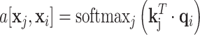(15)

In practice, the dot-product is scaled by a factor , where is the dimensionality of the key. The whole self-attention layer can be written in matrix notation as [68]:

(16)

Expanding on a single attention function, the multi-head attention layer applies attention functions in parallel, effectively learning multiple queries, key and values . Using multiple heads improves the performance of a single attention function. Attention enables the model to learn and effectively store information about the relationships between entries in a sequence in form of matrices. Using any of the attention layers above a single transformer layer is made of a sequence as follows:

• attention layer with residual connection (keeping original information and adding attention onto original input, skip connections also address vanishing gradient)

• layer normalization (stabilizing training)

• N parallel FCNNs for each entry in a sequence with residual connection (introducing non-linearity into the model, skip connections again address vanishing gradient)

• layer normalization (stabilizing training).

Depending on the specific task there are three different types of transformer architectures building upon the transformer layer:

• encoder–decoder (e.g. sequence to sequence modeling like translation)

• encoder (e.g. classification tasks), as in Fig. 2d

• decoder (e.g. text generation).

In PRS, the transformer model makes the same assumptions as the LSTM. In natural language processing, transformer-based models have overtaken LSTMs as state-of-the-art predictors and transformers are thought to be able to model long-range interactions better than LSTMs.

Reyes et al. [70] used an encoder transformer for PRS prediction for Parkinson’s disease. The SNPs are transformed into continuous variable, and starting from the dosage encodings, principal components are computed. Next, a regression model is fitted from these principal components. The residuals between the original regression coefficients from a reference GWAS analysis and the newly fitted regression model are used for each SNP as input. The authors claim removal of confounding effects as a beneficial factor of this approach. Although the proposed transformer model performed best in comparison to other machine learning algorithms, including MLP and LSTM, interpretation of these reported results have to be assessed with care as the datasets, Parkison’s Progression Markers Initiative (PPMI) and Parkinson’s Disease Biomarkers Program (PDBP), are small and no other model was evaluated.

Elmes et al. [71] proposed a transformer trained on a much larger dataset from the UKB to predict risk for gout. Their approach to SNP encoding resembles the tokenization found in natural language processing. All possible SNP combinations of the alleles (e.g. A,C, or A,ins for an insertion) are encoded into 32 numerical input tokens. Together with the SNP token, the SNP’s position is used by the model. Unfortunately, the model’s performance was not assessed against other algorithms. The reported AUC of 0.83 cannot be compared with the AUC of 0.64–0.93 from other models due to differences in study population and SNP data.

Georgantas et al. [72] followed a different approach, combining a linear PRS, a transformer model and gradient boosting. The transformer model learns to pertubate effect sizes of a classical GWAS and these modified effect sizes are then used in a linear PRS. Finally, the output of that linear PRS is combined with a covariate model, a gradient boosting model trained on age, sex and the first 20 principal components of the SNPs, to form a final prediction. The model amplifies effects for SNPs with high effect sizes and reduces small effect sizes. The model was evaluated against machine learning and sta models on 10 different phenotypes in a large cohort derived from UKB data, generally exhibiting an increase in performance but showing no increase in performance for three phenotypes.

A sequence-based model, LSTM, is able to perform fairly well on this sparse representation of the genome, improving performance in comparison to statistical models (see Table 3). The transformer-based models need further evaluation and comparison against additive models. The application of transformers in a similar setting as Yin et al. [60]’s use of CNNs might be worth investigating given the successful application of transformer-based models on short genetic sequences [73].

Table 3.

Performance of LSTM- and transformer-based PRS models for different phenotypes and compared to-state-of-the-art prediction models. The different approaches are compared on phenotypes, the datasets size (n), number of SNPs used in the final model (#SNPs) and on a performance measuring metric. Here, the last column, Compared Method Score, only contains the reported score of the model that performed best in the analysis of the original authors in comparison to their newly proposed deep learning-based model. Values marked with a were read from graphs. Abbreviations: RF = Random forest, lasso = Linear model with L1 regularization, AUC = Area under the curve of the receiver operating characteristic, SBP = Systolic Blood Pressure, TG = Triglycerides, HDL = High-Density Lipoprotein Cholesterol

Study	Phenotype	n	# SNPs	Metric	Score	Compared Method	Compared Method Score
Peng et al. [66]	Alzheimer’s disease	54 162	771	AUC		lasso
	Inflammatory bowel disease	34 652	2481	AUC		lasso
	Type 2 diabetes	159 208	5968	AUC		lasso
	Breast cancer	228 951	3830	AUC		lasso
Reyes et al. [70]	Parkinson’s disease	510	13	AUC		RF
		1068	13	AUC		RF
Elmes et al. [71]	Gout	9000	66 000	AUC	0.83	–	–
Georgantas et al. [72]	SBP	407 008	100 000			XGBoost
	TG	407 008	100 000			XGBoost
	HDL	407 008	100 000			XGBoost

Graph neural networks

Another popular way of modeling data in complex problems is a graph of nodes connected by edges. In the context of genomics, genes could be represented as nodes, while interactions between genes could be modeled as edges. If relationships between nodes are directional, the graph has directed edges, if not they are called undirected. A multigraph can have more than one edge connection between the two nodes, and in a hierarchical graph, nodes in the higher hierarchy can be graphs in a lower level. In a homogenous graph, all nodes and edges are of the same type while in a heterogenous graph, they can be of different types. To process a graph with a neural network, the information of a graph is represented in three matrices. Considering a graph with nodes and edges. First, the adjacency matrix yields information about which nodes are connected to each other via edges; if nodes and are connected, an entry in the matrix is equal to one and zero otherwise. Second, the node embeddings yield information about the individual nodes and are represented by a matrix , where is the dimension of a single node embedding and the number of nodes. The node embedding matrix is the concatenated matrix of all single node embeddings. Similarly, the third matrix of dimension represents the edge embeddings, yielding information about the edge properties. An important property of graphs and GNN is that they are not affected by permutation operations that change the order of the indices of the graphs nodes [69].

In a simple GNN, the embeddings are processed with the adjacency matrix into a hidden representation at the kth layer. The final representation at the final layer is processed by a sigmoid function to yield a probability, as in Fig. 2e.

The graph convolutional network (GCN) [74] focuses on adjacent nodes in its operations. The standard GCN is a spatial operation because it works on the original structure of the graph. If convolutional operations are applied to a transformation of the graph it is called a spectral operation. An aggregating layer in a GCN can be described as [69]:

(17)

where describes a linear transformation, is a non-linear activation function, is the identity matrix and is a -dimensional vector of ones. For the first layer is the node embedding matrix .

There are in general three types of tasks for graph neural networks [69]:

• graph-level tasks (e.g. graph classification)

• node-level tasks (e.g. node classification)

• edge-level tasks (e.g. edge prediction).

In graph-level tasks, the graph node and edge embeddings, and the adjacency matrix are used to classify or predict properties of the whole graph. In node-level tasks, properties of a single node are predicted using information from the rest of the graph’s nodes and edges. In edge-level tasks, the GNN predicts new edges between nodes based on the given embeddings and adjacency.

To process edge-level tasks, the graph is transformed into an edge graph. Here, every edge becomes a node and is connected to the original nodes via edges. In a second step, the nodes of the original graph become edges. The edge-nodes get connected between each other for each common adjacent original node. The resulting graph can then be processed by a GNN.

In PRS prediction, two of the three tasks have been applied. In a graph-level task Li et al. [75] constructed a graph for every individual where the nodes encoded genes and edges connecting the genes were based on a protein-protein interactions. The model was evaluated on multiple phenotypes from the UKB.

In a node-level task, Honda et al. [76] created a graph where every node in the graph represented an individual and was annotated by its SNP genotyping array. Edges between individuals were based on cosine similarity between the SNP genotyping arrays. This model was evaluated on phenotypes from the UKB, BioBank Japan, and the Institute of Rheumatology, Rheumatoid Arthritis cohort [77, 78].

Looking at the predictive performance of GNN PRS, compare Table 4, both approaches improve upon state-of-the-art models, including additive and simple deep learning-based models. The node classification task model, shows more promising results than the graph classification task model. The representation in the GNN-based approaches differs from neural network architectures. Intuitively, the success of the approach depends on the construction of the graph. If the edges in the graph are chosen based on known protein interactions, the model might also be seen as a biologically inspired network. A unique graph representation of the whole dataset is constructed in the node classification task and might be worth further investigations.

Table 4.

Performance of GNN-based PRS models for different phenotypes and compared to state-of-the-art prediction models. The different approaches are compared on phenotypes, the datasets size (n), number of SNPs used in the final model (#SNPs) and on a performance measuring metric. Here, the last column, Compared Method Score, only contains the reported score of the model that performed best in the analysis of the original authors in comparison to their newly proposed deep learning-based model. Values marked with a were read from graphs. The number of SNPs are reported as “?” because no information was given at the time of writing. Abbreviations: AUC = Area under the curve of the receiver operating characteristic, MLP = Multi-layer perceptron

Study	Phenotype	n	# SNPs	Metric	Score	Compared method	Compared method score
Honda et al. [76]	Rheumatoid arthritis	57 605	?	AUC		MLP
	Multiple sclerosis	30 000	?	AUC		PRS-CS
	Psoriasis	30 000	?	AUC		PRSice
	Celiac disease	30 000	?	AUC		MLP
	Atrial fibrillation	30 000	?	AUC		PRS-CS
	Alzheimer’s disease	30 000	?	AUC		MLP
Li et al. [75]	Alzheimer’s diesase	731 800	?	AUC		PLINK
	Multiple sclerosis	731 800	?	AUC		PLINK
	Atrial fibrillation	731 800	?	AUC		LDpred2
	Asthma	731 800	?	AUC		LDpred2
	Rheumatoid arthritis	731 800	?	AUC		PLINK
	Ulcerative colitis	731 800	?	AUC		lassosum2

A gain in performance with a GNN, where the dosage data has been enriched with annotated functions, and the LD of variants, in comparison to a weighted PRS has also been demonstrated by [30]. Similarly to Li et al., a graph was constructed for every individual. In contrast to a gene network, every node represents a single SNP and edges are based on pairwise LD. The features of each node, besides the dosage, included additional biological information such as the location of the SNP and the number of events of histone, open chromatin, polymerase, and transcription factor bindings. However, here the GNN was not able to outperform a state-of-the-art model like lasso.

Autoencoder

The final neural network architecture discussed here is the autoencoder, which is a unsupervised learning algorithm that learns from training examples without the need for labels. Previously, networks were trained in an supervised way using a pair of features and labels for each training example. An autoencoder is a feedforward network consisting of an encoding and decoding part. The encoding layer is typically an FCNN, reducing the dimension to a bottleneck layer of smaller dimension than the input-feature dimension. The decoder part then expands the dimension of the output layer to the same dimension as the input layer; see Fig. 2f. A training example is used as input and the decoder aims to reconstruct it at the output, eliminating the requirement for a label, thereby enabling the unsupervised learning scenario. The internal representation of the training example in the bottleneck layer is then used for downstream tasks due to its reduced dimension [79].

Autoencoders have been used in two ways for PRS development. Firstly as an alternative dimensionality reduction method next to principal component analysis (PCA), effectively enabling the use of more SNPs while keeping the computational cost low. Kaufman et al. [80] compared PCA and autoencoder dimension reduction combined with a MLP and gradient boosting and evaluated these models against state-of-the-art statistical models as well as P-value-based SNP selection in a large cohort on multiple phenotypes. For hypertension and type 2 diabetes, the PCA-based MLP performed best, for height and platelet count, P-value-based SNP selection with a MLP performed best, while for BMI and multiple sclerosis, the additive methods performed best.

A more interesting aspect, however, lies in the use of autoencoders to account for ancestral bias in PRS models. The aforementioned algorithms are for the most part trained on datasets with the majority of individuals being of the same ancestry (mostly Europeans), which yields poor performance on diverse populations with mixed ancestry and a potential bias in precision medicine. Gyawali et al. [81] propose a disentangling autoencoder where the bottleneck representation can be separated into a phenotype-specific part and an ancestry-specific part, on the premise that variations can be observed in these latent representations for different phenotypes and different ancestries, respectively. The final model then uses the phenotype specific representation as well as the original data to form a prediction. The model exhibits highly improved performance on a diverse dataset, as well as improved performance for the minority ancestry group in a predominantly European cohort on Alzheimer’s disease, in comparison to statistical models and a classical MLP. Similarly, Reyes et al. [82] use the latent representation yielded by an autoencoder of summary statistics together with principle components to predict a PRS. The difference here lies in the ancestry specific information being introduced in the loss function. The final model yields a PRS that is comparable throughout ancestries on six UK Biobank traits.

Discussion

This survey of deep learning approaches to PRS construction highlights the potential of these methods for modeling complex genetic architectures. Different architectures each provide unique flexibility in how genetic information is encoded and offer different trade-offs and assumptions about the genotype–phenotype relationship. However, our study has also revealed considerable heterogeneity in the quality and assumptions of implementation and evaluation, from sample size to SNP filtering strategies, and architecture adaption strategies. Compared to sophisticated approaches to PRS based on regularization or Bayesian approaches, deep learning PRS are only emerging as a potentially valuable approach. We identified several challenges and opportunities, listed in Table 5, that offer potential for further improvements into the future.

Table 5.

Key challenges, current state, and future opportunities for deep learning-based polygenic risk scores, as identified in this literature review

Challenge	Current state	Future opportunity
Predictive performance	DL models have better performance than linear PRS in some scenarios	Systematically investigate promising architectures (GNNs, LSTMs, Transformers)
	Performance is inconsistent across diverse architectures, datasets, and phenotypes	Evaluate techniques that improve neural network performance
	Simpler architectures may have limited predictive capacity.	Further explore the integration of prior biological knowledge.
Model benchmarking	Lack of direct comparability due to varied datasets, SNP sets, phenotypes, and evaluation metrics.	Create a common benchmark dataset to allow systematic evaluation of model improvements.
Research reproducibility	DL PRS often have no code, do not share pre-trained weights or available code is challenging to run.	Encourage following existing PRS evaluation guidelines proposed for standard PRS (e.g. Wand et al. [83])
		Encourage open sharing of code, model architectures, and pre-trained weights where feasible.
Model interpretability	—Black-box” nature of many DL models complicates biological understanding.	Assess biological hypotheses with orthogonal evidence
		Explore model basis using explainable AI techniques
		Do not confuse correlation with causation.
Cross-ancestry generalization	Ancestry bias is underexplored in DL-PRS	Assess methods across multi-ancestry, diverse datasets
	Some emerging efforts [72, 75] address ancestry bias, but cannot replicate strong predictive performance across all investigated ancestry groups	Investigate domain adaptation and transfer learning techniques.
	Autoencoder shows promising results in cross-ancestry generalization.

Model benchmarking

As the methods reviewed here were trained on different datasets and address different phenotypes with different sets of SNPs it is hard to compare them, especially since the studies do not all share the same evaluation metric. However, looking at Table 1, it is possible to identify patterns. Although results differ for different phenotypes, a larger dataset (in terms of individuals and features) can boost performance. At the same time, arbitrarily increasing the number of SNPs into the range of SNPs does not improve performance compared with a selection of significant SNPs. An algorithm’s gain in predictive performance with respect to standard models can vary on different phenotypes. This underlines the variety of genetic interactions between phenotypes, indicating that there might not be a universal MLP that can be trained for every phenotype and always yield the best results. Across all neural networks architectures predictive performance increased for breast cancer with respect to compared methods. More complex MLPs that include biological knowledge, sequence-based neural networks and GNNs also exhibit performance improvements for Alzheimer’s disease, schizophrenia and multiple sclerosis. Apart from the choice of model, the dataset itself influences performance independent on its size, as can be seen in Table 3 with Reyes et al. in two different Parkinson’s datasets.

Muneeb et al. [84] showed that a simple MLP-based PRS AUC decreases with increasing heritability and increasing genetic variation, while the classical PRS’s AUC increases, exhibiting completely opposite behavior. The decrease in performance with increasing genetic variation can be attributed to overfitting of the deep learning algorithm. An increase in the number of SNPs does not improve performance of the MLP. This study used simulated data where the heritability and genetic variation can easily be predetermined. In reality, heritability and genetic variation can be hard to determine [85]. Graeley et al. [86] show the decrease in performance with respect to explained variance for MLPs on a simulated dataset; however, the additive model exhibited a decrease in performance as well. Here, an increase of the dataset’s size led to an increase in performance.

As almost none of the authors tested their newly developed models against each other, it would certainly be of interest to see how the models compare in the same dataset. In other areas of neural network research, benchmarking datasets exist to be able to directly compare predictive performance and to track progress (e.g. image classification with the ImageNet dataset [87]). Human genetic data are costly to obtain and require large studies, which pose a challenge that would need to be overcome for the creation of an open benchmarking dataset. Similarly, in the domain of natural language processing, so-called foundation models are developed on large datasets that learn patterns in natural language in general, then for downstream tasks the foundation model can be fine-tuned and shows good predictive performance. Such foundation models have already been developed for DNA sequences [88].

Although deep learning-based PRS models have not been implemented in clinical practice, the adaptation of deep learning-based models could aid in a better stratification of risk as well as identifying more individuals at risk due to better predictive performance in comparison to some of the standard PRS models.

Model interpretability

When interpreting the findings of a deep learning algorithm many authors try to uncover the black box model of a neural network to gain insights about causality and feature importance to find novel causal associations between phenotypes and genotypes. In the case of neural networks interpretability and causality cannot be as easily inferred as with linear regression models and need to be investigated with great care. While there exist several techniques to provide insights into a neural networks such as Grad-CAM, local interpretable model-agnostic explanations, and deep learning important features [89–91] that can find the most influencing features of a model, causality cannot necessarily be inferred with these techniques. The biologically inspired customizations of MLPs also try to make the black box model more interpretable through sparse connection such that weights assigned to a connection might be associated with importance. However, in this case, further hidden layers are highly non-linear and can obscure interpretations of causality. A few authors infer genomic regions of interest through the analysis of the trained deep learning-based algorithms. Chughtai et al. [92] have shown on a simulated example that neural networks do not exhibit strong forms of universality, that is a network trained on similar tasks will learn similar features. It is also emphasized that different architectures as well as the same architecture might learn features differently. This should lead as a guideline that the feature representation trained for a single network should be interpreted with care. A plethora of networks of the same and different architectures should be trained and investigated before interpreting feature importance or weights from neural networks to explain associations between genotypes and phenotypes.

Research reproducibility

Recommendations on the development and evaluation of PRS exist in the literature [83, 93, 94]. While most of the approaches reviewed here follow most of the recommended framework for developing a PRS, there is variation in the evaluation of their findings.

The lack of evaluation guidelines leads to a difficulty in comparing results across approaches. Apart from differences in evaluation, the variety in phenotypes, datasets, and SNPs used makes it difficult to compare the different architectures. Several studies did not evaluate their findings against any of the approaches surveyed in this work. Therefore, it is hard to conclude which approaches might work the best quantitatively as most approaches report improved performance in comparison to additive models or a basic MLP, regular CNNs being an exception.

Looking at the variety of approaches being developed for the non-linear modeling of PRS with neural networks and the observation that most approaches do not build upon similar work or take similar work into account, it is apparent that the best architecture for the input of SNPs has not been found. In contrast to other domains where foundational models are being developed that work well for a given type of data, such as coherent genetic sequences [88], here, we could identify a few approaches that seemingly improve performance over additive models. If a foundational model for the sparse representation of SNPs could be developed, downstream tasks such as PRS prediction could potentially benefit.

Lastly, the lack of comparison between models could also be attributed to difficulty in reproducibility of some of the surveyed models. This could be addressed by sharing implementations of proposed deep learning-based PRS models as well as sharing the trained weights of a model for a specific phenotype. Sharing of weights might be particularly handy when researchers do not have access to the same data sources as the original authors of a specific model.

Biological knowledge shows promise for improvement

A growing trend across polygenic risk scores is the inclusion of biological knowledge to help improve the model’s ability to determine which genetic variants are important for downstream prediction. This is reflected in the deep learning methods examined in this review, where prior knowledge of disease and genetic architecture have been incorporated into several methods either in the types of deep learning architectures used or by incorporating additional information to allow the model to prioritize variants [43, 48, 60].

In the results that have been examined in this review, we observe that the inclusion of biological knowledge appears to improve the results relative to their baseline by between 6% [50] and 30% [46]. However, as discussed above, it is hard to make strong claims as the comparisons are all different.

These trends are in line with a range of developments across polygenic risk scores, in comparison to standard PRS, biological pathway-based PRS exhibit improved performance for disease stratification analyses[95, 96] and are able to improve predictive performance with respect to standard PRS [97]. Additionally, the incorporation of biological knowledge is able to improve cross-ancestry transferability of PRS [98]. This is also hinted at in Sigurddson et al.’ model [99]. However, greater exploration is required to understand whether the prediction improvements we observe from the addition of biological knowledge in neural networks remain when evaluating these models in a robust benchmarking framework.

Outlook

The clinical translation of PRS is rapidly advancing, evidenced by broad interest and an increasing number of clinical trials exploring their utility in personalized medicine. However, the predictive ceiling of conventional PRS has long been constrained by their reliance on linear models, which often fall short of capturing the complex, non-additive nature of genetic risk. While deep learning and artificial intelligence approaches, more broadly have achieved transformative successes in other genomic domains, including sophisticated modeling of DNA sequences and protein structures, these impacts are yet to be fully realized in PRS methodologies. This review has highlighted that if critical hurdles can be overcome, particularly stronger, more consistent benchmarking in model evaluation and greater method reproducibility, deep learning has the potential to redefine the landscape of PRS. Successfully addressing these issues could unlock substantial improvements in predictive accuracy, lead to novel biological insights, and ultimately foster the development of more powerful and equitable PRS for clinical application.

Key Points

• Using deep learning to develop polygenic risk scores enables nonlinear effects to be captured.

• Polygenic risk scores developed using deep learning may show better discriminatory performance than state-of-the-art additive models, though further evaluations are required.

• Incorporating biological knowledge into the neural network architecture shows promising improvement in performance.

• Comparison of performance between proposed models is made difficult by the lack of a common evaluation framework, with models developed and validated on different datasets, SNPs, phenotypes, and metrics. A comprehensive benchmark of deep learning methods within a single testing framework is needed for fair comparison.

Conflict of interest: Gillian Dite works for Rhythm Biosciences on a consultancy basis. The company had no role in the preparation of the manuscript.

References

- 1. Groenendyk JW, Greenland P, Khan SS. Incremental value of polygenic risk scores in primary prevention of coronary heart disease: a review. JAMA Intern Med 2022;182:1082–8. 10.1001/jamainternmed.2022.3171 [DOI] [PubMed] [Google Scholar]
- 2. Khunsriraksakul C, Markus H, Olsen NJ. et al. Construction and application of polygenic risk scores in autoimmune diseases. Front Immunol 2022;13:1–10. 10.3389/fimmu.2022.889296. https://www.frontiersin.org/journals/immunology/articles/10.3389/fimmu.2022.889296/full [DOI] [PMC free article] [PubMed] [Google Scholar]
- 3. Mavaddat N, Michailidou K, Dennis J. et al. Polygenic risk scores for prediction of breast cancer and breast cancer subtypes. Am J Hum Genet 2019;104:21, 1537–34, 6605. 10.1016/j.ajhg.2018.11.002 [DOI] [PMC free article] [PubMed] [Google Scholar]
- 4. Thomas M, Sakoda LC, Hoffmeister M. et al. Genome-wide modeling of polygenic risk score in colorectal cancer risk. Am J Hum Genet 2020;107:432–44. 10.1016/j.ajhg.2020.07.006 [DOI] [PMC free article] [PubMed] [Google Scholar]
- 5. Wang T, Geng J, Zeng X. et al. Exploring causal effects of sarcopenia on risk and progression of Parkinson disease by Mendelian randomization. npj Parkinson’s Dis 2024;10:1, 164–9. 10.1038/s41531-024-00782-3 [DOI] [PMC free article] [PubMed] [Google Scholar]
- 6. Uffelmann E, Huang QQ, Munung NS. et al. Genome-wide association studies. Nat Rev Methods Primers 2021;1.11:1–21. 10.1038/s43586-021-00056-9 [DOI] [Google Scholar]
- 7. Ndong Sima CAA, Step K, Swart Y. et al. Methodologies underpinning polygenic risk scores estimation: a comprehensive overview. Hum Genet 2024. 10.1007/s00439-024-02710-0 10.1007/s00439-024-02710-0 [DOI] [PMC free article] [PubMed] [Google Scholar]
- 8. Duncan L, Shen H, Gelaye B. et al. Analysis of polygenic risk score usage and performance in diverse human populations. Nat Commun 2019;10:3328. 10.1038/s41467-019-11112-0 [DOI] [PMC free article] [PubMed] [Google Scholar]
- 9. Kachuri L, Chatterjee N, Hirbo J. et al. Principles and methods for transferring polygenic risk scores across global populations. Nat Rev Genet 2024;25:8–25. 10.1038/s41576-023-00637-2 [DOI] [PMC free article] [PubMed] [Google Scholar]
- 10. Fadista J, Manning AK, Florez JC. et al. The (in)famous GWAS P-value threshold revisited and updated for low-frequency variants. Eur J Hum Genet: EJHG 2016;24:1202–5. 10.1038/ejhg.2015.269 [DOI] [PMC free article] [PubMed] [Google Scholar]
- 11. Collister JA, Liu X, Clifton L. Calculating polygenic risk scores (PRS) in UK Biobank: a practical guide for epidemiologists. Front Genet 2022;13:818574. 10.3389/fgene.2022.818574 [DOI] [PMC free article] [PubMed] [Google Scholar]
- 12. Privé F, Vilhjálmsson BJ, Aschard H. et al. Making the most of clumping and thresholding for polygenic scores. Am J Hum Genet 2019;105:1213–21. 10.1016/j.ajhg.2019.11.001 [DOI] [PMC free article] [PubMed] [Google Scholar]
- 13. Vilhjálmsson BJ, Yang J, Finucane HK. et al. Modeling linkage disequilibrium increases accuracy of polygenic risk scores. Am J Hum Genet 2015;97:576, 1537–92, 6605. 10.1016/j.ajhg.2015.09.001 [DOI] [PMC free article] [PubMed] [Google Scholar]
- 14. Privé F, Arbel J, Vilhjálmsson BJ. LDpred2: better, faster, stronger. Bioinf (Oxf) 2021;36:5424–31. 10.1093/bioinformatics/btaa1029 [DOI] [PMC free article] [PubMed] [Google Scholar]
- 15. Mak TSH, Porsch RM, Choi SW. et al. Polygenic scores via penalized regression on summary statistics. Genet Epidemiol 2017;41:469–80. 10.1002/gepi.22050 [DOI] [PubMed] [Google Scholar]
- 16. Lloyd-Jones LR, Zeng J, Sidorenko J. et al. Improved polygenic prediction by Bayesian multiple regression on summary statistics. Nat Commun 2019;10:5086. 10.1038/s41467-019-12653-0 [DOI] [PMC free article] [PubMed] [Google Scholar]
- 17. Ge T, Chen C-Y, Ni Y. et al. Polygenic prediction via Bayesian regression and continuous shrinkage priors. Nat Commun 2019;10:1776. 10.1038/s41467-019-09718-5 [DOI] [PMC free article] [PubMed] [Google Scholar]
- 18. Melo F. Area under the ROC curve. In: Dubitzky W, Wolkenhauer O, Cho K-H et al (eds), Encyclopedia of Systems Biology. New York, NY: Springer, 2013, 38–39. 10.1007/978-1-4419-9863-7_209. [DOI] [Google Scholar]
- 19. Nagelkerke NJD. A note on a general definition of the coefficient of determination. Biometrika 1991;78:691–2. 10.1093/biomet/78.3.691 [DOI] [Google Scholar]
- 20. Alpaydin E. Introduction to Machine Learning. en-US MIT Press, 2014. https://mitpress.mit.edu/9780262028189/introduction-to-machine-learning/. [Google Scholar]
- 21. Ramachandran P, Zoph B, Le QV. Searching for activation functions. arXiv preprint 2017. arXiv:1710.05941. 10.48550/arXiv.1710.05941 [DOI]
- 22. Hornik K. Approximation capabilities of multilayer feedforward networks. Neural Netw 1991;4:251–7. 10.1016/0893-6080(91)90009-T [DOI] [Google Scholar]
- 23. Fukushima K. Visual feature extraction by a multilayered network of analog threshold elements. IEEE Trans Syst Sci Cybernet 1969;5:322–33. 10.1109/TSSC.1969.300225 [DOI] [Google Scholar]
- 24. Lu Z, Pu H, Wang F. et al. The expressive power of neural networks: a view from the width. In: Curran Associates Inc. (eds.), Proceedings of the 31st International Conference on Neural Information Processing Systems. Red Hook, NY, USA, 2017, 6232–6240. 10.48550/arXiv.1709.02540 [DOI]
- 25. LeCun Y, Bengio Y, Hinton G. Deep learning. Nature 2015;521:436–44. 10.1038/nature14539 [DOI] [PubMed] [Google Scholar]
- 26. Perelygin V, Kamelin A, Syzrantsev N. et al. Deep learning captures the effect of epistasis in multifactorial diseases. Front Med 2025;11:1–11. 10.3389/fmed.2024.1479717 https://www.frontiersin.org/journals/medicine/articles/10.3389/fmed.2024.1479717/full [DOI] [PMC free article] [PubMed] [Google Scholar]
- 27. Cordell HJ. Epistasis: what it means, what it doesn’t mean, and statistical methods to detect it in humans. Hum Mol Genet 2002;11:2463–8. 10.1093/hmg/11.20.2463 [DOI] [PubMed] [Google Scholar]
- 28. Badré A, Zhang L, Muchero W. et al. Deep neural network improves the estimation of polygenic risk scores for breast cancer. J Hum Genet 2021;66:359–69. 10.1038/s10038-020-00832-7 [DOI] [PubMed] [Google Scholar]
- 29. Hinton GE, Srivastava N, Krizhevsky A. et al. Improving neural networks by preventing co-adaptation of feature detectors. arXiv:1207.0580. arXiv preprint 2012. https://arxiv.org/abs/1207.0580v1 [Google Scholar]
- 30. Zhou X, Chen Y, Ip FCF. et al. Deep learning-based polygenic risk analysis for Alzheimer’s disease prediction. Commun Med 2023;3:1–20. 10.1038/s43856-023-00269-x [DOI] [PMC free article] [PubMed] [Google Scholar]
- 31. Saykin AJ, Shen L, Foroud TM. et al. Alzheimer’s disease neuroimaging initiative biomarkers as quantitative phenotypes: genetics core aims, progress, and plans. Alzheimers Dement 2010;6:265–73. 10.1016/j.jalz.2010.03.013 [DOI] [PMC free article] [PubMed] [Google Scholar]
- 32. Zhou X, Chen Y, Mok KY. et al. Identification of genetic risk factors in the Chinese population implicates a role of immune system in Alzheimer’s disease pathogenesis. Proc Natl Acad Sci U S A 2018;115:1697–706. 10.1073/pnas.1715554115 [DOI] [PMC free article] [PubMed] [Google Scholar]
- 33. Zhou X, Chen Y, Ip FCF. et al. Genetic and polygenic risk score analysis for Alzheimer’s disease in the Chinese population. Alzheimer’s Dement (Amsterdam, Netherlands) 2020;12:e12074. 10.1002/dad2.12074 [DOI] [PMC free article] [PubMed] [Google Scholar]
- 34. Kim SB, Kang JH, Cheon M. et al. Penalised neural network with weight correlation descent for predicting polygenic risk score. medRxiv preprint 2023. 10.1101/2023.05.23.23290438. https://www.medrxiv.org/content/10.1101/2023.05.23.23290438v1 [DOI]
- 35. Kim SB, Kang JH, Cheon M. et al. Stacked neural network for predicting polygenic risk score. Sci Rep 2024;14:11632. 10.1038/s41598-024-62513-1 [DOI] [PMC free article] [PubMed] [Google Scholar]
- 36. Sudlow C, Gallacher J, Allen N. et al. UK Biobank: an open access resource for identifying the causes of a wide range of complex diseases of middle and old age. PLoS Med 2015;12:e1001779. 10.1371/journal.pmed.1001779 [DOI] [PMC free article] [PubMed] [Google Scholar]
- 37. Bycroft C, Freeman C, Petkova D. et al. The UK Biobank resource with deep phenotyping and genomic data. Nature 2018;562:203–9. 10.1038/s41586-018-0579-z [DOI] [PMC free article] [PubMed] [Google Scholar]
- 38. Health Examinees Study Group . The health examinees (HEXA) study: rationale, study design and baseline characteristics. Asian Pacific J Cancer Prevent: APJCP 2015;16:1591–7. 10.7314/apjcp.2015.16.4.1591 [DOI] [PubMed] [Google Scholar]
- 39. Huang S, Ji X, Cho M. et al. DL-PRS: a novel deep learning approach to polygenic risk scores. Preprint 2021. 10.21203/rs.3.rs-423764/v1. https://www.researchsquare.com/article/rs-423764/v1 [DOI]
- 40. Regan EA, Hokanson JE, Murphy JR. et al. Genetic epidemiology of COPD (COPDGene) study design. COPD 2010;7:32–43. 10.3109/15412550903499522 [DOI] [PMC free article] [PubMed] [Google Scholar]
- 41. Hou C, Xu B, Hao Y. et al. Development and validation of polygenic risk scores for prediction of breast cancer and breast cancer subtypes in Chinese women. BMC Cancer 2022;22:374. 10.1186/s12885-022-09425-3 [DOI] [PMC free article] [PubMed] [Google Scholar]
- 42. Wen W, Shu X-O, Guo X. et al. Prediction of breast cancer risk based on common genetic variants in women of east Asian ancestry. Breast Cancer Res: BCR 2016;18:124. 10.1186/s13058-016-0786-1 [DOI] [PMC free article] [PubMed] [Google Scholar]
- 43. Nguyen ND, Jin T, Wang D. Varmole: a biologically drop-connect deep neural network model for prioritizing disease risk variants and genes. Bioinformatics 2021;37:1772–5. 10.1093/bioinformatics/btaa866 [DOI] [PMC free article] [PubMed] [Google Scholar]
- 44. Tibshirani R. Regression shrinkage and selection via the lasso. J R Stat Soc B Methodol 1996;58:267–88. [Google Scholar]
- 45. Wang D, Liu S, Warrell J. et al. Comprehensive functional genomic resource and integrative model for the human brain. Science (New York, NY) 2018;362:eaat8464. 10.1126/science.aat8464 [DOI] [PMC free article] [PubMed] [Google Scholar]
- 46. Liu L, Meng Q, Weng C. et al. Explainable deep transfer learning model for disease risk prediction using high-dimensional genomic data. PLoS Comput Biol 2022;18:e1010328. 10.1371/journal.pcbi.1010328 [DOI] [PMC free article] [PubMed] [Google Scholar]
- 47. Clark SA, van der Werf J. Genomic best linear unbiased prediction (gBLUP) for the estimation of genomic breeding values. In: Gondro C, van der Werf J, Hayes B (eds.), Genome-Wide Association Studies and Genomic Prediction. Methods in Molecular Biology, Vol. 1019. Totowa, NJ, USA: Humana Press, 2013, 321–30. 10.1007/978-1-62703-447-0_13. 10.1007/978-1-62703-447-0_13 [DOI] [PubMed] [Google Scholar]
- 48. van Hilten A, Kushner SA, Kayser M. et al. GenNet framework: interpretable deep learning for predicting phenotypes from genetic data. Commun Biol 2021;4:1, 2399–9, 3642. 10.1038/s42003-021-02622-z [DOI] [PMC free article] [PubMed] [Google Scholar]
- 49. Purcell SM, Moran JL, Fromer M. et al. A polygenic burden of rare disruptive mutations in schizophrenia. Nature 2014;506:185–90. 10.1038/nature12975 [DOI] [PMC free article] [PubMed] [Google Scholar]
- 50. Sigurdsson AI, Louloudis I, Banasik K. et al. Deep integrative models for large-scale human genomics. Nucleic Acids Res 2023;51:e67. 10.1093/nar/gkad373 [DOI] [PMC free article] [PubMed] [Google Scholar]
- 51. LeCun Y, Bengio Y. Convolutional networks for images, speech, and time series. In: Arbib MA (ed.), The Handbook of Brain Theory and Neural Networks, 255–8. Cambridge, MA: USA MIT Press, 1998. [Google Scholar]
- 52. Kwon O-S, Hong M, Kim T-H. et al. Genome-wide association study-based prediction of atrial fibrillation using artificial intelligence. Open Heart 9:2022, e001898. 10.1136/openhrt-2021-001898 [DOI] [PMC free article] [PubMed] [Google Scholar]
- 53. Bae J, Logan PE, Acri DJ. et al. A simulative deep learning model of SNP interactions on chromosome 19 for predicting Alzheimer’s disease risk and rates of disease progression. Alzheimers Dement 2023;19:5690–9. 10.1002/alz.13319 [DOI] [PMC free article] [PubMed] [Google Scholar]
- 54. Bellot P, de los Campos G, Pérez-Enciso M. Can deep learning improve genomic prediction of complex human traits? Genetics 2018;210:809–19. 10.1534/genetics.118.301298 [DOI] [PMC free article] [PubMed] [Google Scholar]
- 55. Xu Y, Vuckovic D, Ritchie SC. et al. Machine learning optimized polygenic scores for blood cell traits identify sex-specific trajectories and genetic correlations with disease. Cell Genomics 2022;2:1–12. 10.1016/j.xgen.2021.100086 https://www.cell.com/cell-genomics/abstract/S2666-979X(21)00107-5 [DOI] [PMC free article] [PubMed] [Google Scholar]
- 56. Segura MA, Bini G, Krithara A. et al. Machine learning methods applied to classify complex diseases using genomic data. bioRxiv preprint 2024. 10.1101/2024.03.18.585541. https://www.biorxiv.org/content/10.1101/2024.03.18.585541v1 [DOI]
- 57. Moore C, Sambrook J, Walker M. et al. The INTERVAL trial to determine whether intervals between blood donations can be safely and acceptably decreased to optimise blood supply: study protocol for a randomised controlled trial. Trials 2014;15:363. 10.1186/1745-6215-15-363 [DOI] [PMC free article] [PubMed] [Google Scholar]
- 58. Consortium IMSG, Hafler DA, Compston A. et al. Risk alleles for multiple sclerosis identified by a genomewide study. N Engl J Med 2007;357:851–62. 10.1056/NEJMoa073493 [DOI] [PubMed] [Google Scholar]
- 59. Buda M, Maki A, Mazurowski MA. A systematic study of the class imbalance problem in convolutional neural networks. Neural Netw 2018;106:249–59. 10.1016/j.neunet.2018.07.011 [DOI] [PubMed] [Google Scholar]
- 60. Yin B, Balvert M, van der Spek RAA. et al. Using the structure of genome data in the design of deep neural networks for predicting amyotrophic lateral sclerosis from genotype. Bioinformatics 2019;35:i538–47. 10.1093/bioinformatics/btz369 [DOI] [PMC free article] [PubMed] [Google Scholar]
- 61. Van Rheenen W, Pulit SL, Dekker AM. et al. Project MinE: study design and pilot analyses of a large-scale whole-genome sequencing study in amyotrophic lateral sclerosis. Eur J Hum Genet 2018;26:1537–46. 10.1038/s41431-018-0177-4 [DOI] [PMC free article] [PubMed] [Google Scholar]
- 62. Agarwal V, Shendure J. Predicting mRNA abundance directly from genomic sequence using deep convolutional neural networks. Cell Rep 2020;31. 10.1016/j.celrep.2020.107663. https://www.cell.com/cell-reports/abstract/S2211-1247(20)30616-1 [DOI] [PubMed] [Google Scholar]
- 63. Kelley DR, Reshef YA, Bileschi M. et al. Sequential regulatory activity prediction across chromosomes with convolutional neural networks. Genome Res 2018;28. Company: Cold Spring Harbor Laboratory Press Distributor: Cold Spring Harbor Laboratory Press Institution: Cold Spring Harbor Laboratory Press Label: Cold Spring Harbor Laboratory Press Publisher: Cold Spring Harbor Lab PMID: 29588361, 739–750. issn: 1088–9051, 1549–5469. 10.1101/gr.227819.117 [DOI] [PMC free article] [PubMed] [Google Scholar]
- 64. Avsec Ž, Agarwal V, Visentin D. et al. Effective gene expression prediction from sequence by integrating long-range interactions. Nat Methods 2021;18:1196–203. 10.1038/s41592-021-01252-x [DOI] [PMC free article] [PubMed] [Google Scholar]
- 65. Hochreiter S, Schmidhuber J. Long short-term memory. Neural Comput 1997;9:1735–80. 10.1162/neco.1997.9.8.1735 [DOI] [PubMed] [Google Scholar]
- 66. Peng J, Bao Z, Li J. et al. DeepRisk: a deep learning approach for genome-wide assessment of common disease risk. Fund Res 2024;4:752–60. 10.1016/j.fmre.2024.02.015. https://www.sciencedirect.com/science/article/pii/S2667325824001171 [DOI] [PMC free article] [PubMed] [Google Scholar]
- 67. Zhao WX, Zhou K, Li J. et al. A survey of large language models. arXiv:2303.18223. arXiv preprint 2024. 10.48550/arXiv.2303.18223. http://arxiv.org/abs/2303.18223 [DOI]
- 68. Vaswani A, Shazeer N, Parmar N. et al. Attention is all you need. In: Curran Associates Inc. (eds.), Proceedings of the 31st International Conference on Neural Information Processing Systems. Red Hook, NY, USA, 2017, 6000–10. 10.48550/arXiv.1706.03762 [DOI]
- 69. Prince SJ. Understanding Deep Learning. The MIT Press, 2023. http://udlbook.com [Google Scholar]
- 70. Reyes DM, Kim M, Chao H. et al. Genomics transformer for diagnosing Parkinson’s disease. IEEE-EMBS International Conference on Biomedical and Health Informatics 2022. 2022. 10.1109/bhi56158.2022.9926815 [DOI] [PMC free article] [PubMed] [Google Scholar]
- 71. Elmes K, Benavides-Prado D, Tan NO. et al. SNVformer: an attention-based deep neural network for GWAS data. bioRxiv preprint 2022. 10.1101/2022.07.07.499217. https://www.biorxiv.org/content/10.1101/2022.07.07.499217v2 [DOI]
- 72. Georgantas C, Kutalik Z, Richiardi J. Delphi: a deep-learning framework for polygenic risk prediction. medRxiv preprint 2024. 10.1101/2024.04.19.24306079. https://www.medrxiv.org/content/10.1101/2024.04.19.24306079v1 [DOI]
- 73. Jumper J, Evans R, Pritzel A. et al. Highly accurate protein structure prediction with AlphaFold. Nature 2021;596:583–9. 10.1038/s41586-021-03819-2 [DOI] [PMC free article] [PubMed] [Google Scholar]
- 74. Kipf TN, Welling M. Semi-supervised classification with graph convolutional networks. International Conference on Learning Representations 2017. 10.48550/arXiv.1609.02907. http://arxiv.org/abs/1609.02907 [DOI]
- 75. Li H, Zeng J, Snyder MP. et al. PRS-net: Interpretable polygenic risk scores via geometric learning. In: Ma J (ed.), International Conference on Research in Computational Molecular Biology, pp. 377–80. Cham: Springer Nature Switzerland, 2024. 10.1101/2024.02.13.580211 [DOI]
- 76. Honda S, Ikari K, Terao C. et al. Polygenic risk score for predicting the development of autoimmune diseases using graph convolutional networks: a model development and validation study. Annals of the Rheumatic Diseases 2024;83:538–39. https://papers.ssrn.com/abstract=4695065 [Google Scholar]
- 77. Yamanaka H, Tanaka E, Nakajima A. et al. A large observational cohort study of rheumatoid arthritis, IORRA: providing context for today’s treatment options. Mod Rheumatol 2020;30:1–6. 10.1080/14397595.2019.1660028 [DOI] [PubMed] [Google Scholar]
- 78. Nagai A, Hirata M, Kamatani Y. et al. Overview of the BioBank Japan project: study design and profile. J Epidemiol 2017;27:S2–8. 10.1016/j.je.2016.12.005 [DOI] [PMC free article] [PubMed] [Google Scholar]
- 79. Bank D, Koenigstein N, Giryes R. Autoencoders. arXiv: 2003.05991. arXiv preprint 2021. 10.48550/arXiv.2003.05991 http://arxiv.org/abs/2003.05991 [DOI]
- 80. Kaufman H, Hochenberg Y, Linial M. et al. DROP-DEEP: dimensionality reduction for polygenic risk score using DEEP learning approach. medRxiv preprint 2024. 10.1101/2024.05.01.24306609. https://www.medrxiv.org/content/10.1101/2024.05.01.24306609v1 [DOI]
- 81. Gyawali PK, Le Guen Y, Liu X. et al. Improving genetic risk prediction across diverse population by disentangling ancestry representations. Commun Biol 2023;6:1–9. 10.1038/s42003-023-05352-6 [DOI] [PMC free article] [PubMed] [Google Scholar]
- 82. Machado Reyes D, Bose A, Karavani E. et al. FairPRS: adjusting for admixed populations in polygenic risk scores using invariant risk minimization. Biocomputing 2023. World Scientific, 2022, 198–208. 10.1142/9789811270611_0019. https://www.worldscientific.com/doi/10.1142/9789811270611_0019 [DOI] [PMC free article] [PubMed] [Google Scholar]
- 83. Wand H, Lambert SA, Tamburro C. et al. Improving reporting standards for polygenic scores in risk prediction studies. Nature 2021;591:211–9. 10.1038/s41586-021-03243-6 [DOI] [PMC free article] [PubMed] [Google Scholar]
- 84. Muneeb M, Feng SF, Henschel A. Heritability, genetic variation, and the number of risk SNPs effect on deep learning and polygenic risk scores AUC Proceedings of the 14th International Conference on Bioinformatics and Biomedical Technology. ICBBT ‘22. New York, NY, USA Association for Computing Machinery, 2022, 65–71. 10.1145/3543377.3543387. https://dl.acm.org/doi/10.1145/3543377.3543387. [DOI] [Google Scholar]
- 85. Zuk O, Hechter E, Sunyaev SR. et al. The mystery of missing heritability: genetic interactions create phantom heritability. Proc Natl Acad Sci 2012;109:1193–8. 10.1073/pnas.1119675109 [DOI] [PMC free article] [PubMed] [Google Scholar]
- 86. Grealey J, Abraham G, Méric G. et al. Deep learning for polygenic prediction: the role of heritability, interaction type and sample size. medRxiv preprint 2024. 10.1101/2024.10.25.24316156. https://www.medrxiv.org/content/10.1101/2024.10.25.24316156v1 [DOI]
- 87. Deng J, Dong W, Socher R. et al. ImageNet: a large-scale hierarchical image database. 2009 IEEE Conference on Computer Vision and Pattern Recognition. 2009, 248–255. 10.1109/CVPR.2009.5206848 [DOI]
- 88. Dalla-Torre H, Gonzalez L, Mendoza-Revilla J. et al. Nucleotide Transformer: building and evaluating robust foundation models for human genomics. Nature Methods 2025;22: 287–97. 10.1038/s41592-024-02523-z [DOI] [PMC free article] [PubMed] [Google Scholar]
- 89. Ribeiro MT, Singh S, Guestrin C. “Why should I trust you?”: explaining the predictions of any classifier. In Proceedings of the 22nd ACM SIGKDD International Conference on Knowledge Discovery and Data Mining. New York, NY, USA: Association for Computing Machinery, 2016, 1135–44. 10.48550/arXiv.1602.04938 [DOI]
- 90. Shrikumar A, Greenside P, Kundaje A. Learning important features through propagating activation differences. In International Conference on Machine Learning. Sydney, NSW, Australia: JMLR.org, 2017, 3145–53. https://arxiv.org/abs/1704.02685v2
- 91. Selvaraju RR, Cogswell M, Das A. et al. Grad-CAM: visual explanations from deep networks via gradient-based localization. Int J Comput Vis 2020.. arXiv:1610.02391;128:336–59 1573–1405. 10.1007/s11263-019-01228-7 [DOI] [Google Scholar]
- 92. Chughtai B, Chan L, Nanda N. A toy model of universality: reverse engineering how networks learn group operations. In International Conference on Machine Learning 2023, 6243–67. 10.48550/arXiv.2302.03025 [DOI]
- 93. Choi SW, Mak TS-H, O’Reilly PF. Tutorial: a guide to performing polygenic risk score analyses. Nat Protoc 2020;15:2759–72. 10.1038/s41596-020-0353-1 [DOI] [PMC free article] [PubMed] [Google Scholar]
- 94. Pain O, Glanville KP, Hagenaars SP. et al. Evaluation of polygenic prediction methodology within a reference-standardized framework. PLoS Genet 2021;17:e1009021. 10.1371/journal.pgen.1009021 [DOI] [PMC free article] [PubMed] [Google Scholar]
- 95. Choi SW, García-González J, Ruan Y. et al. PRSet: pathway-based polygenic risk score analyses and software. PLoS Genet 2023;19:e1010624, 1553–7404. 10.1371/journal.pgen.1010624 [DOI] [PMC free article] [PubMed] [Google Scholar]
- 96. Dehestani M, Liu H, Sreelatha AAK. et al. Mitochondrial and autophagy-lysosomal pathway polygenic risk scores predict Parkinson’s disease. Mol Cell Neurosci 2022;121:103751. 10.1016/j.mcn.2022.103751 [DOI] [PubMed] [Google Scholar]
- 97. Dass SAH, McCracken K, Pokhvisneva I. et al. A biologically-informed polygenic score identifies endophenotypes and clinical conditions associated with the insulin receptor function on specific brain regions. EBioMedicine 2019;42:188–202. 10.1016/j.ebiom.2019.03.051 [DOI] [PMC free article] [PubMed] [Google Scholar]
- 98. Amadeus S, Cenggoro TW, Budiarto A. et al. A Design of Polygenic Risk Model with deep learning for colorectal cancer in multiethnic Indonesians. In: Procedia Computer Science. 5th International Conference on Computer Science and Computational Intelligence 2020 179, 2021,. 632–639. 10.1016/j.procs.2021.01.049 [DOI] [Google Scholar]
- 99. Sigurdsson AI, Ravn K, Winther O. et al. Improved prediction of blood biomarkers using deep learning. medRxiv preprint 2022. 10.1101/2022.10.27.22281549 [DOI]