Effect Measures in Prevalence Studies

Abstract

There is still considerable confusion and debate about the appropriate methods for analyzing prevalence studies, and a number of recent papers have argued that prevalence ratios are the preferred method and that prevalence odds ratios should not be used. These arguments assert that the prevalence ratio is obviously the better measure and the odds ratio is “unintelligible.” They have often been accompanied by demonstrations that when a disease is common the prevalence ratio and the prevalence odds ratio may differ substantially. However, this does not tell us which measure is the more valid to use. In fact, the prevalence odds ratio a) estimates the incidence rate ratio with fewer assumptions than are required for the prevalence ratio; b) can be estimated using the same methods as for the odds ratio in case–control studies, namely, the Mantel–Haenszel method and logistic regression; and c) provides practical, analytical, and theoretical consistency between analyses of a prevalence study and prevalence case–control analyses based on the same study population. For these reasons, the prevalence odds ratio will continue to be one of the standard methods for analyzing prevalence studies and prevalence case–control studies.

Although the methods for analyzing incidence studies (and incidence case–control studies) are now well established, there is still considerable confusion and debate about the appropriate methods for analyzing prevalence studies (and prevalence case–control studies). In particular, it has been argued that prevalence ratios are the preferred method and that prevalence odds ratios (PORs) should not be used. In this article I argue that PORs should continue to be one of the standard methods for analyzing such studies. I briefly review the relationship between incidence and prevalence studies and then discuss the relative merits of using PORs and prevalence ratios.

Incidence Studies

Table 1 shows the findings of a hypothetical incidence study of 20,000 persons followed for 10 years (Pearce 2003). Three measures of disease incidence are commonly used in incidence studies (Pearce 1993): the person-time incidence rate, the incidence proportion, and the incidence odds. These all involve the same numerator: the number of incident cases of disease (b). They differ in whether their denominators represent person-years at risk (Y₀), persons at risk (N₀), or survivors (d).

Table 1.

Findings from a hypothetical cohort study of 20,000 persons followed for 10 years.

	Exposed	Nonexposed	Ratio
Cases	1,813 (a)	952 (b)
Noncases	8,187 (c)	9,048 (d)
Total population	10,000 (N1)	10,000 (N0)
Person-years	90,635 (Y1)	95,163 (Y0)
Incidence rate	0.0200 (I1)	0.0100 (I0)	2.00
Incidence proportion (average risk)	0.1813 (R1)	0.0952 (R0)	1.90
Incidence odds	0.2214 (O1)	0.1052 (O0)	2.11

The person-time incidence rate is a measure of the disease occurrence per unit population time and has the reciprocal of time as its dimension. In this example (Table 1), there were 952 cases of disease diagnosed in the nonexposed group during the 10 years of follow-up, which involved a total of 95,163 person-years, and the person-time incidence rate, b/Y₀ = I₀, was 952/95,163 = 0.0100 (or 1,000 per 100,000 person-years).

The incidence proportion, or average risk, is a second measure of disease occurrence and is the proportion of study subjects who experience the outcome of interest at any time during the follow-up period. In this instance, there were 952 incident cases among the 10,000 people in the nonexposed group, and the incidence proportion, b/N₀ = R₀, was therefore 952/10,000 = 0.0952 over the 10-year follow-up period. When the outcome of interest is rare over the follow-up period (e.g., an incidence proportion < 10%), then the incidence proportion is approximately equal to the incidence rate multiplied by the length of time that the population has been followed (in the example this product is 0.1000, whereas the incidence proportion is 0.0952).

A third possible measure of disease occurrence is the incidence odds (Greenland 1987), which is the ratio of the number of people who experience the outcome (b) to the number of people who do not experience the outcome (d). As for the incidence proportion, the incidence odds is dimensionless, but it is necessary to specify the time period over which it is being measured. In this example, the incidence odds, b/d = O₀, is 952/9,048 = 0.1052. When the outcome is rare over the follow-up period, the incidence odds is approximately equal to the incidence proportion.

Corresponding to these three measures of disease occurrence, there are three principal ratio measures of effect that can be used in incidence studies (Pearce 1993): the rate ratio, the risk ratio, and the incidence odds ratio.

The rate ratio is the ratio of the incidence rate in the exposed group (a/Y₁) to that in the nonexposed group (b/Y₀). In the example in Table 1, the incidence rates are 0.02 per person-year in the exposed group and 0.01 per person-year in the nonexposed group, and the rate ratio is therefore 2.00. A second commonly used effect measure is the risk ratio, which is the ratio of the incidence proportion in the exposed group (a/N₁) to that in the nonexposed group (b/N₀). In this example, the risk ratio is 0.1813/0.0952 = 1.90. A third possible effect measure is the incidence odds ratio, which is the ratio of the incidence odds in the exposed group (a/c) to that in the non-exposed group (b/d). In this example, the odds ratio is 0.2214/0.1052 = 2.11.

These three multiplicative effect measures are sometimes referred to under the generic term of relative risk. In this example, they all show that the rate (or risk, or odds) of developing the disease under study is about twice as high in the exposed group as in the nonexposed group, but their precise estimates vary (2.00, 1.90, and 2.11, respectively). Thus, they are all approximately equal when the disease is rare during the follow-up period (e.g., an incidence proportion < 10%). However, although the rate ratio and (to a lesser extent) the risk ratio are both commonly used for analyzing incidence studies, the odds ratio has been severely criticized as an effect measure (Greenland 1987; Miettinen and Cook 1981) and has little intrinsic meaning in incidence studies.

Prevalence Studies

Incidence studies are the ideal method for studying disease occurrence because they involve collecting and analyzing all the relevant information on the source population, and we can get better information on when exposure and disease occurred. However, these types of studies involve lengthy periods of follow-up and many resources in terms of both time and funding, and it may be difficult to identify incident cases of nonfatal chronic conditions such as diabetes or asthma. Furthermore, in some instances we may be more interested in factors that affect the current burden of disease in the population. Consequently, although incidence studies are usually preferable, there is also an important role for prevalence studies, for practical reasons and because such studies enable the assessment of the level of morbidity and the population “disease burden” for a nonfatal condition (Pearce 2003; Thompson et al. 1998).

Measures of effect in prevalence studies.

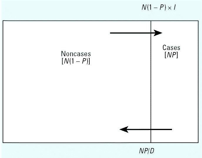
Figure 1 shows the relationship between incidence and prevalence of disease in a “steady-state” population. Suppose we denote the prevalence of disease in the study population by P, and we assume that the population is in a steady state (stationary) over time (in that the numbers within each subpopulation defined by exposure, disease, and covariates do not change with time)—this usually requires that incidence rates and exposure and disease status are unrelated to the immigration and emigration rates and population size, and that average disease duration (D) does not change over time. Then the prevalence odds is equal to the incidence rate (I) times D (Alho 1992):

Figure 1. Relationship between prevalence and incidence in a steady-state population. Abbreviations: D, duration; I, incidence; N, population; P, prevalence.

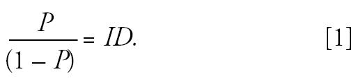Now suppose that we compare two populations (indexed by 1 = exposed and 0 = non-exposed) that both satisfy the above conditions. Then, the prevalence odds is directly proportional to the disease incidence, and the POR satisfies the equation

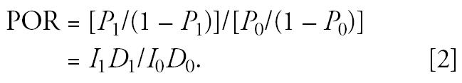An increased POR may thus reflect the influence of factors that increase the duration of disease as well as those that increase disease incidence. A difference in prevalence between two groups could depend entirely on differences in disease duration (e.g., because of factors that prolong or exacerbate symptoms) rather than differences in incidence. However, in the special case where the average duration of disease is the same in the exposed and non-exposed groups (i.e., exposure has no effect on duration), then the POR satisfies the equation

That is, under the above assumptions, the POR directly estimates the incidence rate ratio. However, the prevalence ratio (P₁/P₀) only approximately satisfies this equation provided that the disease is rare and therefore (1 − P₁) and (1 − P₀) are close to 1.0.

Of course, such a steady-state population will rarely exist in practice, but it will be approximated in situations where disease incidence and the relevant exposures are not changing markedly over time (provided the other assumptions specified above are met). This is also conditional on other risk factors (e.g., age) because even when incidence is independent of age, prevalence will often be age dependent (Keiding 1991, 2000), and these other risk factors therefore need to be controlled for in the analysis.

Table 2 shows data from a prevalence study of 20,000 people, with the data derived from Table 1 using Equation 2 above. This is based on the assumptions that, for both populations, the incidence rate and population size are constant over time, that the average duration of disease is 5 years, and that there is no migration of people with the disease into or out of the population (such assumptions may not be realistic but are made here for purposes of illustration). In this situation, the number of cases who “lose” the disease each year is balanced by the number of new cases generated from the source population. For example, in the nonexposed group, there are 476 prevalent cases, and 95 (20%) of these “lose” their disease each year; this is balanced by the 95 people who develop the disease each year (0.0100 of the susceptible population of 9,524 people). One example of such a condition would be childhood asthma, where most children “lose” the condition after a few years (5 years on average, in this hypothetical example) whereas other children are acquiring the condition for the first time; meanwhile, the age-specific prevalence remains relatively constant. With the additional assumption that the average duration of disease is the same in the exposed and nonexposed groups, then the POR (2.00) validly estimates the incidence rate ratio (Table 1).

Table 2.

Findings from a hypothetical prevalence study of 20,000 persons.

	Exposed	Nonexposed	Ratio
Cases	909 (a)	476 (b)
Noncases	9,091 (c)	9,524 (d)
Total population	10,000 (N1)	10,000 (N0)
Prevalence	0.0909 (P1)	0.0476 (P0)	1.91
Prevalence odds	0.1000 (O1)	0.0500 (O0)	2.00

Data are derived from Table 1 using Equation 2 based on the assumptions that, for both populations, the incidence rate and population size are constant over time, that the average duration of disease is 5 years, and that there is no migration of people with the disease into or out of the population.

Of course, when the above steady-state assumptions are not met, which will frequently be the case, then both the POR and the prevalence ratio will differ from the incidence rate ratio (Thompson et al. 1998), and which measure is more “valid” will be highly specific to the population, exposure, and disease. However, as the population pattern approaches steady state, the POR increasingly estimates the incidence rate ratio with greater validity than does the prevalence ratio.

Prevalence case–control studies.

Just as an incidence case–control study can be used to obtain the same findings as a full incidence study, a prevalence case–control study can be used to obtain the same findings as a full prevalence study in a more efficient manner. In particular, if obtaining exposure information is difficult or costly (e.g., if it involves lengthy interviews, or serum samples), then it may be more efficient to conduct a prevalence case–control study by obtaining exposure information on all of the prevalent cases and a sample of controls selected at random from the noncases. For example, suppose a nested case–control study is conducted in the study population (Table 2), involving all of the 1,385 prevalent cases and a group of 1,385 controls selected from the noncases (Table 3). The ratio of exposed to nonexposed controls will estimate the exposure odds (b/d) of the noncases, and the odds ratio obtained in the prevalence case–control study will therefore estimate the POR in the source population (2.00), which in turn estimates the incidence rate ratio, provided that the above assumptions are satisfied in the exposed and non-exposed populations.

Table 3.

Findings from a hypothetical prevalence case–control study based on the population represented in Table 1.

	Exposed	Nonexposed	Ratio
Cases	909 (a)	476 (b)
Controls	676 (c)	709 (d)
Prevalence odds	1.34 (O1)	0.67 (O0)	2.00

Which Effect Measure Should We Use?

So which effect measure should we use to analyze a prevalence study?

Reasons for using the POR.

There are a number of reasons why the use of the POR is attractive. First, although this is not always the case, prevalence studies are frequently conducted to learn more about the risk factors for a disease; that is, they are conducted to find out how to prevent the incidence of the disease. In this situation, incidence is the effect measure of interest. As shown above, provided that certain (admittedly restrictive) assumptions are met, the POR provides an unbiased estimate of the incidence rate ratio. On the other hand, for the prevalence ratio to provide such an unbiased estimate requires that all of the same assumptions are met, plus the additional assumption that the disease is rare. Thus, when the incidence rate ratio is the real effect measure of interest, the POR will estimate this with fewer assumptions than are required for the prevalence ratio.

A second reason often given for using the POR is ease of computation, because the POR can be calculated using standard methods for case–control studies such as the Mantel–Haenszel (1959) method or logistic regression (Rothman and Greenland 1998). This has obvious practical advantages because of the widespread availability and use of appropriate computer packages. Logistic regression or the proportional hazards model can also be used to estimate the prevalence ratio, but this is not straightforward and estimation may be intractable in the presence of many covariates (Thompson et al. 1998). However, this “problem” with using the prevalence ratio is more imaginary than real because standard methods can be used to model prevalences, just as they can be used to model risks (both prevalence and risk are expressed as a proportion; Tables 1 and 2). These include the Mantel–Haenszel method for risk/prevalence (pure count data; Rothman and Greenland 1998), and (exponential) risk regression (Zocchetti et al. 1995). It is sometimes argued that (exponential) risk regression is inappropriate because it may yield predicted values of the prevalence that are < 0 or > 1 (Lee 1995), but this is rarely a problem in practice (Rothman and Greenland 1998). It is also argued that only a few explanatory variables can be accommodated because cross-classification will yield many cells without at least one prevalence case (Lee 1995). However, the Mantel–Haenszel method for risk:prevalence ratios is relatively robust, just as the Mantel–Haenszel method for odds ratios is (Rothman and Greenland1998). Similarly, (exponential) risk regression using maximum likelihood methods performs just as well as logistic regression does for estimating odds ratios. Thus, this “computational” argument for using PORs rather than prevalence ratios is invalid.

However, there is a third reason for using PORs that is rarely mentioned: that it provides consistency between prevalence studies and prevalence case–control studies based on the same population. It is frequently the case that a prevalence study is conducted first to identify cases and noncases for a chronic condition such as asthma or diabetes, and that all of the identified cases and a control sample (chosen from the noncases) are then selected for further investigation. For example, phase I of the International Study of Asthma and Allergies in Childhood (Asher et al. 1995; Pearce et al. 1993) involved asthma prevalence studies in children in 155 centers in 56 countries (Beasley et al. 1998), and the initial prevalence studies were in many instances used as basis for more detailed prevalence case–control studies (e.g., Wickens et al. 1999). Such an approach is practical and logical because it is not necessary to obtain detailed information (e.g., more detailed questionnaires, skin prick testing, blood tests) for the entire study population; rather, it is more efficient to obtain it for all of the cases and a sample of the noncases. In prevalence case–control studies the prevalence odds ratio is the standard effect measure, just as in an incidence case–control study the (incidence) odds ratio is the standard effect measure (Morgenstern and Thomas 1993; Pearce 1998). Furthermore, provided that controls are sampled without bias, the POR in a prevalence case–control study will provide an unbiased estimate of the POR that would have been obtained in a full prevalence study based on the same source population. There are therefore obvious benefits, both practically and conceptually, with using the POR in a full prevalence study to provide theoretic and analytic consistency between the analysis of the full prevalence study and any prevalence case–control analyses that may be conducted in the same population.

Reasons for using the prevalence ratio.

So why doesn’t everyone use the POR? One argument is that when a disease is common, then the POR and the prevalence ratio may differ greatly, and there may also be differences in the nature and extent of confounding and effect modification (Thompson et al. 1998). However, the fact that the two methods give different results when the disease is common (they give very similar results when the disease is rare) does not tell us which measure is more appropriate to use. Rather, it emphasizes the importance of using the measure that is most appropriate for the task.

A second argument is that “the odds ratio is incomprehensible” (Lee 1994). However, this assertion is based on a misquoting of the literature (e.g., Greenland 1987), which shows that the odds ratio is not a meaningful effect measure in a cohort study. This tells us nothing about the use of the odds ratio in other contexts. In particular, the odds ratio is the standard effect measure in an (incidence) case–control study and, provided that the controls have been selected appropriately, will estimate the incidence rate ratio without the need for any rare disease assumption (Pearce 1993). Similarly, as shown above, provided a number of more restrictive assumptions are made, the POR is not only a meaningful effect measure in a prevalence study, but will also estimate the incidence rate ratio with fewer assumptions than are required for the prevalence ratio. What is incomprehensible and inappropriate for use in a cohort study may be quite comprehensible and appropriate for use in a incidence case–control study or a prevalence study.

A third and related argument is that the prevalence ratio has greater “natural intelligibility” (Axelson et al. 1994; Lee and Chia 1993; Thompson et al. 1998). For example, Lee and Chia (1993) argue that “whereas PR [prevalence ratio] is easy to interpret and to communicate, POR lacks intelligibility.” However, what is most intelligible and interpretable to one person may not be so to another. Moreover, the most intelligible measures may not be the most valid. For example, using the same logic, one might argue that the ratio of the percentage of cases exposed to the percentage of controls exposed in an (incidence) case–control study (the exposure ratio) is more intelligible and easier to communicate than is the (exposure) odds ratio. Moreover, it could be argued that there is good evidence for this given the confusion about the odds ratio, and what it is estimating in an (incidence) case–control study, that stretches back for nearly 50 years (Pearce 1993). Nevertheless, the odds ratio is the standard effect measure to use in an (incidence) case–control study despite its lack of “natural intelligibility.”

A final argument for using the prevalence ratio is that sometimes we are interested in prevalence itself, rather than incidence, and that in this situation the prevalence ratio is clearly the effect measure of interest—for example, when we are concerned about the public health burden of disease. This argument clearly has merit, albeit with the qualification that in this situation it is often the absolute value of prevalence and the prevalence difference that are of greatest interest, rather than the prevalence ratio.

Conclusion

A number of authors have argued that the prevalence ratio is the preferable effect measure to use in prevalence studies. The case for using the prevalence ratio essentially reduces to the assertion that it is obviously the better measure whereas the odds ratio is “unintelligible,” and that when a disease is common the prevalence ratio and the POR may differ substantially. However, although such analyses are valuable in indicating how much the two measures may diverge, and under what circumstances, they do not solve the problem as to which measure is the most appropriate to use. A more valid argument is that the prevalence ratio is the effect measure of interest when we are interested in the public health burden of disease, although in this situation the absolute prevalence and the prevalence difference are usually of more interest. However, when we are interested in disease etiology, the POR a) estimates the incidence rate ratio with fewer assumptions than are required for the prevalence ratio; b) can be estimated using the same methods as for the odds ratio in case–control studies, namely, the Mantel–Haenszel method and logistic regression; and c) provides practical, analytical, and theoretical consistency between analyses of a prevalence study and those of a prevalence case–control study based on the same study population. For these reasons, the POR will continue to be one of the standard methods for analyzing prevalence studies and prevalence case–control studies.

References

- Alho JM. On prevalence, incidence, and duration in general stable populations. Biometrics. 1992;48:587–592. [PubMed] [Google Scholar]
- Asher I, Keil U, Anderson HR, Beasley R, Crane J, Martinez F, et al. International study of asthma and allergies in childhood (ISAAC): rationale and methods. Eur Respir J. 1995;8:483–491. doi: 10.1183/09031936.95.08030483. [DOI] [PubMed] [Google Scholar]
- Axelson O, Fredriksson M, Ekberg K. Use of the prevalence ratio v the prevalence odds ratio as a measure of risk in cross-sectional studies. Occup Environ Med. 1994;51:574. doi: 10.1136/oem.51.8.574. [DOI] [PMC free article] [PubMed] [Google Scholar]
- Beasley R, Keil U, Von Mutius E, Pearce N. Worldwide variation in prevalence of symptoms of asthma, allergic rhinoconjunctivitis and atopic eczema: ISAAC. The International Study of Asthma and Allergies in Childhood (ISAAC) Steering Committee. Lancet. 1998;351:1225–1232. [PubMed] [Google Scholar]
- Greenland S. Interpretation and choice of effect measures in epidemiologic analyses. Am J Epidemiol. 1987;125:761–768. doi: 10.1093/oxfordjournals.aje.a114593. [DOI] [PubMed] [Google Scholar]
- Keiding N. Age-specific incidence and prevalence: a statistical perspective. J R Statist Soc. 1991;154:371–412. [Google Scholar]
- Keiding N. 2000. Incidence-prevalence relationships. In: Encyclopedia of Epidemiological Methods (Gail M, Benichou J, eds). Chichester, UK:Wiley, 433–437.
- Lee J. Odds ratio or relative risk for cross-sectional data. Int J Epidemiol. 1994;23:201–203. doi: 10.1093/ije/23.1.201. [DOI] [PubMed] [Google Scholar]
- Lee J. Estimation of prevalence rate ratios from cross-sectional data: a reply. Int J Epidemiol. 1995;24:1065–1066. doi: 10.1093/ije/24.5.1064. [DOI] [PubMed] [Google Scholar]
- Lee J, Chia KS. Estimation of prevalence rate ratios for cross-sectional data: an example in occupational epidemiology. Br J Ind Med. 1993;50:861–862. doi: 10.1136/oem.50.9.861. [DOI] [PMC free article] [PubMed] [Google Scholar]
- Mantel N, Haenszel W. Statistical aspects of the analysis of data from retrospective studies of disease. J Natl Cancer Inst. 1959;22:719–748. [PubMed] [Google Scholar]
- Miettinen OS, Cook EF. Confounding: essence and detection. Am J Epidemiol. 1981;114:593–603. doi: 10.1093/oxfordjournals.aje.a113225. [DOI] [PubMed] [Google Scholar]
- Morgenstern H, Thomas D. Principles of study design in environmental epidemiology. Environ Health Perspect. 1993;101(suppl 4):23–38. doi: 10.1289/ehp.93101s423. [DOI] [PMC free article] [PubMed] [Google Scholar]
- Pearce N. What does the odds ratio estimate in a case-control study? Int J Epidemiol. 1993;22:1189–1192. doi: 10.1093/ije/22.6.1189. [DOI] [PubMed] [Google Scholar]
- Pearce N. The four basic epidemiologic study types. J Epidemiol Biostat. 1998;3:171–177. [Google Scholar]
- Pearce N. 2003. A Short Introduction to Epidemiology. Wellington, New Zealand:Centre for Public Health Research.
- Pearce N, Weiland S, Keil U, Langridge P, Anderson HR, Strachan D, et al. Self-reported prevalence of asthma symptoms in children in Australia, England, Germany and New Zealand: an international comparison using the ISAAC protocol. Eur Respir J. 1993;6:1455–1461. [PubMed] [Google Scholar]
- Rothman KJ, Greenland S. 1998. Modern Epidemiology. 2nd ed. Philadelphia:Lippincott-Raven.
- Thompson ML, Myers JE, Kriebel D. Prevalence odds ratio or prevalence ratio in the analysis of cross sectional data: what is to be done? Occup Environ Med. 1998;55:272–277. doi: 10.1136/oem.55.4.272. [DOI] [PMC free article] [PubMed] [Google Scholar]
- Wickens K, Crane J, Kemp T, Lewis S, D’Souza W, Sawyer G, et al. Family size, infections and asthma in New Zealand children. Epidemiology. 1999;10:699–705. [PubMed] [Google Scholar]
- Zocchetti C, Consonni D, Bertazzi PA. Estimation of prevalence rate ratios from cross-sectional data. Int J Epidemiol. 1995;24:1064–1105. doi: 10.1093/ije/24.5.1064. [DOI] [PubMed] [Google Scholar]