

Abstract
We determined the secular trend in blood lead levels in a cohort of 321 children born in Mexico City between 1987 and 1992. Blood lead level was measured every 6 months during a 10-year period. We modeled the effect of yearly air lead concentration nested within the calendar year in which the child was born, family use of lead-glazed pottery, socioeconomic status, year in which the child was born, age of the child at the time of blood lead measurement, place of residence, and an indicator variable for subjects with complete or incomplete blood lead values. The yearly mean of air lead of the Valley of Mexico decreased from its highest level of 2.80 μg/m3 in 1987 to 0.07 μg/m3 in 2002. The contribution of air lead to blood lead according to year of birth was strongest for subjects born in 1987 and fell to nearly zero for children born in 1992. The geometric mean of the entire cohort rose from 8.4 μg/dL in the first year of life to 10.1 μg/dL in the second and decreased thereafter until it reached 6.4 μg/dL at 10 years of age. Children of families who used lead-glazed ceramics had blood lead levels 18.5% higher than did children of nonusing families. Children who belonged to the lowest socioeconomic levels had blood lead levels 32.2% higher than did those of highest socioeconomic levels. Children who lived in the northeast part of the city had blood lead levels 10.9% higher compared with those who lived in the southwest.
Keywords: air lead, blood lead, children, gasoline, lead-glazed ceramic, Mexico City
Population lead exposure has been one of the main environmental health problems in Mexico (Albert and Badillo 1991; Friberg and Vahter 1983; Olaiz et al. 1996; Romieu et al. 1994; Rothenberg et al. 1993). Several standards have been published in the last decade to restrict emissions and reduce the exposure to this metal. Lead in gasoline, one of the main sources of environmental exposure eliminated in the past decade, was reduced by > 98.5% between 1986 and 1997. In September 1997 it was eliminated from all gasoline sold in the metropolitan zone of the Valley of Mexico. Thanks to the elimination of this source, from 1988 to 2002 the mean lead air level was reduced from 2.80 μg/m3 to 0.07 μg/m3 (Departamento del Distrito Federal 1998; Driscoll et al. 1992; Romieu et al. 1994). Notwithstanding the success in reducing air lead, there are still other sources of population exposure, such as fixed industrial sources that contaminate restricted zones in their surroundings and lead-glazed ceramics that affect most of the population (Hernandez-Avila et al. 1991, 1996; Navarrete-Espinosa et al. 2000; Olaiz et al. 1996).
The results of several cross-sectional studies from the population in Mexico City performed during the last decade reveal a reduction in blood lead levels, an indicator of environmental lead exposure.
However, these data do not allow evaluation of the effect of the reduction of environmental exposure across time. For this reason, our objective in this work was to determine the secular trend in blood lead concentrations of a cohort of children evaluated every 6 months during their first 10 years of life. We also quantified the relative contribution of several other sources of exposure to this metal to their blood lead levels. Nevertheless, because of the difficulty in specifying and measuring the different lead sources, the data of this study can only provide the lower limit of the contribution of each source.
Materials and Methods
Subjects.
We recruited 502 pregnant women attending the prenatal clinic at 12 weeks of pregnancy at the National Institute of Perinatology in Mexico City. They all signed an informed consent form approved by the ethics committee of the institute. Only 383 of the children born to these women fulfilled the inclusion criteria: 5-min Apgar score ≥ 7, birth weight > 2,000 g, gestation age ≥ 36 weeks, without major or minor congenital anomalies or being the product of multiple birth. Of these children, 62 were lost to follow-up between 1 and 6 months after birth.
We followed 321 children, born between 1987 and 1992, through structured interviews of the parents and with psychometric tests and blood lead determinations every 6 months from delivery. Table 1 presents the characteristics of the sample. Parents were informed of potential sources of lead, routes of exposure, toxicity of lead, and some ways to avoid it. They also received nutritional and hygienic orientation. None of the children received chelation therapy.
Table 1.
Characteristics of tested versus not-tested subjects.
| Subjects included (n = 321)
|
Subjects not tested (n = 62)
|
||
|---|---|---|---|
| Characteristics | No. (%) | No. (%) | p-Valuea |
| Sex | |||
| Male | 174 (54.2) | 32 (51.6) | 0.781 |
| Female | 147 (45.8) | 30 (48.4) | |
| SES | |||
| Lowest | 52 (16.2) | 8 (12.9) | 0.714 |
| Medium | 189 (58.9) | 36 (58.1) | |
| Highest | 80 (24.9) | 18 (29.0) | |
| Clay pot useb | |||
| Yes | 128 (39.9) | 24 (46.2) | 0.447 |
| No | 193 (60.1) | 28 (53.8) | |
| Cohort size (year)c | |||
| 1987 | 38 (11.8) | 13 (21.0) | |
| 1988 | 68 (21.2) | 16 (25.8) | |
| 1989 | 34 (10.6) | 2 (3.2) | |
| 1990 | 60 (18.7) | 14 (22.6) | |
| 1991 | 49 (15.3) | 5 (8.1) | |
| 1992 | 72 (22.4) | 12 (19.3) | |
Fisher’s exact test or Pearson chi-square exact probability, subjects tested versus subjects not tested.
In some not-tested subjects, there was no information about clay pot use.
Year in which child was born.
Blood lead measurements.
We drew venous blood into purple-top Vacutainers that contained ethylenediamine tetraacetic acid. Blood samples were analyzed in duplicate by anodic stripping voltammetry, at the Environmental Associates Laboratories (ESA Labs; Chelmsford, MA, USA). Samples with mean duplicate values < 5 μg/dL were reanalyzed via atomic absorption spectrometry. Quality control information is provided elsewhere (Rothenberg et al. 1994). ESA Labs is a reference laboratory for the Centers for Disease Control and Prevention’s Blood Lead Laboratory Reference System (Atlanta, GA, USA) and participates in the Commonwealth of Pennsylvania Department of Health Blood Lead Proficiency Testing Program (Exton, PA, USA).
For the statistical analysis, we calculated the arithmetic mean of the biannual concentrations of lead determined during each year of the child’s life and natural log transformed the means for use in modeling.
Air lead measurements.
We extracted air lead information from the Statistical Compendium of the System of Atmospheric Monitoring of the Metropolitan Zone of the Valley of Mexico (MZVM), 1986–2002 (Departamento del Distrito Federal 2003). Air lead concentrations were obtained through the Automatic Network of Atmospheric Monitoring (ANAM) of the MZVM that started operations in 1986 (Departamento del Distrito Federal 2003).
At present, the ANAM includes 19 stations with manual equipment. The network records in particle filters the concentrations of total suspended particles, particles < 10 μm, and metals such as lead. The ANAM generates a 24-hr sample every 6 days. Air lead concentrations were analyzed by atomic absorption spectrometry.
We used air lead data collected at three air monitoring stations that reported the most complete data during the study period. In the selection of these stations, we also looked for a geographic area with high contamination levels (Xalostoc, an industrial zone placed behind a smelter in the northeast sector of the city), a zone with intermediate levels (Merced, a mixed high-density commercial–residential zone with heavy vehicular traffic in the center of the city), and a zone with low atmospheric lead levels (Pedregal, a low-density, upscale residential zone in the southwest of the city).
We calculated each year’s average of 3-month means for each station’s air lead data. We used natural-log–transformed yearly means for statistical modeling.
Other variables.
Children were placed into separate subcohorts according to the year in which they were born. To avoid collinearity of air lead over time with age of child, air lead was nested within each of the resulting six subcohorts in subsequent analyses, instead of being used as a separate independent variable. The resulting coefficients for the six nested air lead variables thus reflected the effect of lead on secular trend of air lead on subcohort blood lead across all ages instead of on blood lead according to age of child.
Socioeconomic status (SES) was computed by equally weighting the sum of three separate nine-point scales measuring education and occupation of the head of the family and the total family income based on integral multiples of the minimum wage. SES of the families ranged from low-low to lower-upper. For this analysis, we collapsed the resulting sum of the three SES scales into only three categories: low SES (the low-low and middle-low categories), upper-lower and lower-middle SES, and middle-middle and higher SES. The information about family use of lead-glazed ceramic was obtained during the pregnancy and was coded as a “yes” or “no” response on the questionnaire. Place of residence was fixed into one of the three nonoverlapping zones in which the air monitoring stations were located based on family residential address. The northeast sector, represented by the Xalostoc air monitoring station (with the highest air lead values), was used as the omitted dummy variable in the residential analysis. We recorded the family residential address at recruitment and at varying times after. We created a dummy variable indicating whether the address changed during the participation of the child in the study. We coded as “unchanged address” the 53 subjects (16.5% of the sample) whose post-natal address was unverifiable but who contributed postnatal lead data. Because not all subjects had blood lead data for every age, we created a dummy variable indicating complete or incomplete (missing data at one or more ages) blood lead for each subject.
Statistical analyses.
We used Fisher’s exact tests (StatXact 5; Cytel Software Corp., Cambridge, MA, USA) to compare frequencies of sex, SES, and leaded ceramic ware use between subjects included in the analysis and subjects whose mother was recruited into the study but who failed to present to the study after 1 month of age. We compared the same variables with Fisher’s exact tests to determine if there were significant differences between subjects with complete lead data from 1 to 10 years of age and those with missing data points for 1 or more years. We used t-tests for independent groups to determine differences in blood lead concentration at each age between subjects with complete lead data and those with missing data at one or more ages. We applied a Kruskal-Wallis chi-square test with exact probabilities (StatXact) to determine if there was a significant association between SES and use of lead-glazed ceramic ware.
We used the SPSS version 11.5 (SPSS, Inc., Chicago, IL, USA) linear mixed-effects models procedure to analyze the data set as a repeated-measures, unbalanced analysis of variance design using heterogeneous first-order autoregressive covariance structure of the repeated measure, natural log blood lead at each age (10 levels), and a fixed-effects air lead (mean annual air lead concentration for each calendar year of the study) nested within the subcohort according to the calendar year in which the child was born (six levels). The other fixed variables were year in which the child was born (six levels), family SES (three categories), use of lead-glazed ceramic ware (two levels), indicator variables for place of residence (three variables), and an indicator variable for subjects with complete or one or more missing blood lead values.
We selected the covariance structure of the repeated-measures variable by inspection of the covariance matrix and by the use of information criteria of the model as a whole. The restricted log likelihood measures the fit of the data to the model, and Bozdogan’s criterion (Bozdogan 2000) provides an alternate measure of fit, penalizing the fit measure according to the number of parameters in the model. We used the heterogeneous first-order autoregressive structure because it was in accordance with the observed unrestricted covariance matrix and maximized the fit measures.
We used the Sidak procedure to adjust two-tailed p-values in all post hoc multiple comparisons. We used the Jonckheere-Terpstra test in post hoc analyses of the trend in blood lead across year of birth at each age. We used exact p-values as calculated by StatXact.
Results
Table 1 shows the differences between included and excluded data. There were no differences between the groups in sex, SES, or use of lead-glazed ceramics. Only 31.2% (n = 100) of subjects provided lead data at all 10 ages; 48.3% (n = 155) of subjects had three or fewer missing lead values. The proportion of children who used lead-glazed ceramic ware was lower in the group of subjects with incomplete data (Table 2). The proportion of children living in the southwest sector was lower and in the northeast sector was higher in children with incomplete data. The geometric mean of blood lead (GMPb) was also significantly higher in the incomplete group at almost all ages except at 1, 2, and 4 years of age (Table 3).
Table 2.
Characteristics of subjects with complete versus incomplete data.
| With complete data (n = 100)
|
With incomplete data (n = 221)
|
||
|---|---|---|---|
| Characteristics | No. (%) | No. (%) | p-Valuea |
| Sex | |||
| Male | 51 (51.0) | 123 (55.6) | 0.469 |
| Female | 49 (49.0) | 98 (44.4) | |
| SES | |||
| Lowest | 10 (10.0) | 42 (19.0) | 0.126 |
| Medium | 63 (63.0) | 127 (57.5) | |
| Highest | 27 (27.0) | 52 (23.5) | |
| Clay pot use | |||
| Yes | 48 (48.0) | 79 (35.7) | 0.048 |
| No | 52 (52.0) | 142 (64.3) | |
| Cohort size (year born)b | |||
| 1987 | 10 (10.0) | 28 (12.7) | |
| 1988 | 17 (17.0) | 51 (23.1) | |
| 1989 | 13 (13.0) | 21 (9.5) | |
| 1990 | 16 (16.0) | 44 (19.9) | |
| 1991 | 16 (16.0) | 33 (14.9) | |
| 1992 | 28 (28.0) | 44 (19.9) | |
| Place of residence | |||
| Southwest | 48 (48.0) | 71 (32.1) | 0.008 |
| Center | 33 (33.0) | 77 (34.8) | |
| Northeast | 19 (19.0) | 73 (33.1) | |
Fisher’s exact test or Pearson chi-square exact probability, complete data versus incomplete data.
Year in which child was born.
Table 3.
Differences in GMPb between subjects with complete and incomplete data.
| With complete data
|
With incomplete data
|
||||
|---|---|---|---|---|---|
| Age (years) | Mean ± SD | No. | Mean ± SD | No. | p-Valuea |
| 1 | 9.2 ± 1.7 | 100 | 9.3 ± 1.7 | 202 | 0.762 |
| 2 | 10.5 ± 1.8 | 100 | 11.0 ± 1.7 | 164 | 0.480 |
| 3 | 9.3 ± 1.7 | 100 | 10.9 ± 1.6 | 118 | 0.014 |
| 4 | 8.4 ± 1.6 | 100 | 9.4 ± 1.7 | 107 | 0.101 |
| 5 | 7.4 ± 1.6 | 100 | 9.5 ± 1.6 | 81 | 0.001 |
| 6 | 6.6 ± 1.6 | 100 | 8.1 ± 1.6 | 65 | 0.008 |
| 7 | 6.2 ± 1.6 | 100 | 7.8 ± 1.5 | 64 | 0.002 |
| 8 | 5.5 ± 1.6 | 100 | 6.6 ± 1.6 | 54 | 0.022 |
| 9 | 5.2 ± 1.6 | 100 | 6.8 ± 1.5 | 45 | 0.001 |
| 10 | 4.9 ± 1.6 | 100 | 6.2 ± 1.5 | 34 | 0.014 |
t-Tests for independent groups.
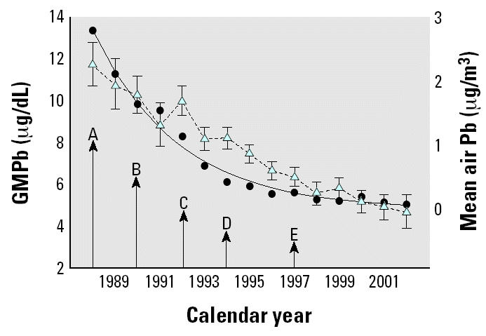
Figure 1 shows the time course of lead in air and lead in blood of the entire cohort according to the year of the study. In this graph, blood lead is confounded by age and year because in the early years of the study only younger children were available and in the later years of the study only older children contributed data. Yearly average air lead concentration decreased from its highest level of 2.8 μg/m3 in 1987 to 0.07 μg/m3 in 2002. Dates of important changes in gasoline lead content are indicated by the arrows in Figure 1.
Figure 1. Yearly GMPb concentration with geometric 95% CIs (blue triangles, dashed line) of entire cohort and yearly mean air lead concentration with natural log air lead regression line (black circles, solid line) as a function of calendar year. Regression adjusted R2 = 0.96, indicating adequate specification of air lead by natural log transformation in statistical modeling. Arrows indicate important reductions in permitted lead content of gasoline in Mexico: A, 0.5–1.0 mL/gal; B, 0.3–0.54 mL/gal; C, 0.2–0.3 mL/gal; D, 0.1–0.2 mL/gal; E, 0.0 mL/gal.
SES, the age of the child at the time of blood lead measurement, the year in which the child was born, family use of lead-glazed ceramic, and the yearly mean of air lead of the Valley of Mexico significantly predicted the children’s blood lead levels (p ≤ 0.001) as well as place of residence and having missing data (p < 0.05; Table 4).
Table 4.
Estimates of fixed effects.a
| Parameter | Estimate [ln(μg/dL)] | df | p-Value | 95% CI |
|---|---|---|---|---|
| Intercept | 1.615 | 1073.84 | 0.000 | 1.388 to 1.842 |
| SES | ||||
| Low | 0.280 | 368.84 | 0.000 | 0.157 to 0.402 |
| Medium | 0.088 | 368.84 | 0.046 | 0.002 to 0.175 |
| High | 0.000b | |||
| Age (years) | ||||
| 1 | 0.274 | 1140.60 | 0.000 | 0.120 to 0.428 |
| 2 | 0.456 | 1131.48 | 0.000 | 0.315 to 0.596 |
| 3 | 0.405 | 1009.02 | 0.000 | 0.279 to 0.531 |
| 4 | 0.339 | 880.97 | 0.000 | 0.229 to 0.449 |
| 5 | 0.309 | 796.55 | 0.000 | 0.210 to 0.408 |
| 6 | 0.199 | 623.72 | 0.000 | 0.116 to 0.283 |
| 7 | 0.188 | 524.82 | 0.000 | 0.114 to 0.261 |
| 8 | 0.084 | 439.96 | 0.011 | 0.019 to 0.148 |
| 9 | 0.034 | 316.94 | 0.167 | −0.014 to 0.082 |
| 10 | 0.000b | |||
| Year born | ||||
| 1987 | 0.437 | 677.11 | 0.000 | 0.266 to 0.608 |
| 1988 | 0.472 | 620.64 | 0.000 | 0.316 to 0.627 |
| 1989 | 0.328 | 535.15 | 0.000 | 0.151 to 0.506 |
| 1990 | 0.205 | 512.58 | 0.014 | 0.042 to 0.368 |
| 1991 | 0.194 | 516.75 | 0.033 | 0.016 to 0.371 |
| 1992 | 0.000b | |||
| Clay pot use | ||||
| Yes | 0.170 | 364.6 | 0.000 | 0.096 to 0.244 |
| No | 0.000b | |||
| Locationc | ||||
| Southwest | −0.115 | 3670.0 | 0.013 | −0.205 to −0.024 |
| Center | −0.074 | 379.11 | 0.125 | −0.169 to 0.021 |
| Air lead (year born) | ||||
| 1987 | 0.213 | 924.26 | 0.000 | 0.114 to 0.312 |
| 1988 | 0.166 | 834.78 | 0.000 | 0.086 to 0.246 |
| 1989 | 0.162 | 986.16 | 0.002 | 0.061 to 0.261 |
| 1990 | 0.116 | 998.51 | 0.005 | 0.035 to 0.196 |
| 1991 | 0.143 | 1004.30 | 0.001 | 0.056 to 0.229 |
| 1992 | −0.003 | 1191.42 | 0.934 | −0.083 to 0.076 |
| Incomplete blood lead | 0.089 | 360.95 | 0.023 | 0.012 to 0.167 |
Dependent variable was ln(blood lead).
This parameter is set to zero because it is redundant.
Northeast (Xalostoc) is the omitted dummy variable.
The contribution of air lead to lifetime blood lead according to year of birth was estimated in the mixed model (Table 4). It was strongest for subjects born in 1987 (each natural log decrease in air lead was accompanied by a 23.7% decrease in blood lead concentration across the first 10 years of life) and fell to nearly zero in the children born in 1992. Post hoc contrasts showed that the most important difference in lifetime blood lead was between the part of the cohort born in 1987 and 1988 compared with the part of the cohort born in 1991 and 1992 (Figure 2). The difference in lifetime blood lead concentration between the two subcohorts was 43.0% [t = 5.919, degrees of freedom (df) = 725.9, p < 0.0005]. It is notable that completely unleaded gasoline was introduced into Mexico City in the last quarter of 1990. Leaded gasoline completely disappeared from the Mexico City market in 1997 (Figure 1). There was a significant decrease (p < 0.01) in the percentage of children with blood lead ≥ 10 μg/dL (the current Mexican action limit) across year of birth (subcohort) during each of the first 7 years of life (Table 5).
Figure 2. Effect of year of birth on GMPb. Shown are geometric means with 95% CIs estimated from the mixed model.
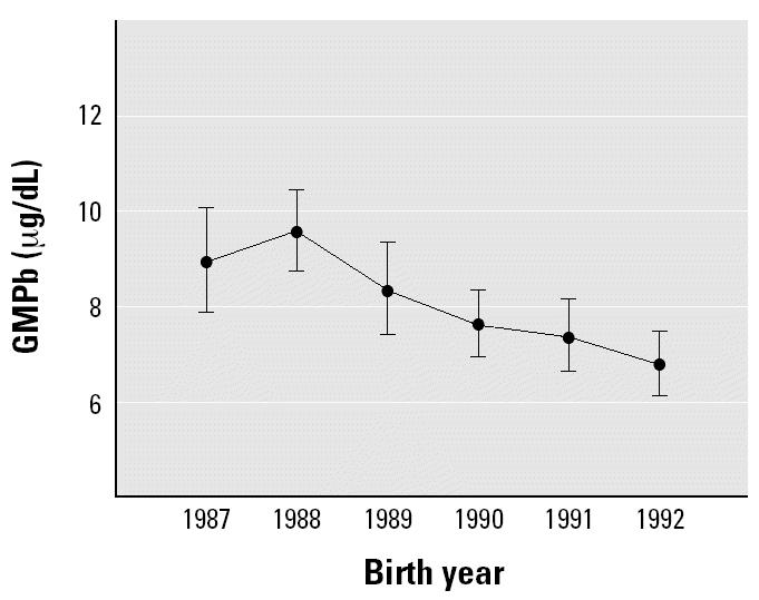
Table 5.
Percentage of children with blood lead levels ≥ 10 μg/dL during the first 10 years of life by year of birth.
| Year
|
||||||||
|---|---|---|---|---|---|---|---|---|
| Age (years) | 1987 | 1988 | 1989 | 1990 | 1991 | 1992 | J–T testa | p-Value |
| 1 | 80.0 | 74.6 | 42.4 | 38.6 | 41.3 | 19.1 | 13360.5 | < 0.0005 |
| 2 | 89.3 | 89.7 | 55.5 | 52.0 | 38.5 | 26.7 | 9450.5 | < 0.0005 |
| 3 | 73.1 | 78.0 | 84.0 | 43.2 | 38.7 | 19.6 | 6757.5 | < 0.0005 |
| 4 | 76.9 | 68.6 | 45.5 | 21.6 | 21.2 | 16.7 | 6111.0 | < 0.0005 |
| 5 | 76.2 | 68.6 | 12.5 | 25.0 | 25.8 | 15.2 | 4788.0 | < 0.0005 |
| 6 | 47.6 | 37.9 | 18.8 | 15.2 | 25.0 | 14.3 | 4794.0 | 0.003 |
| 7 | 42.1 | 33.3 | 17.6 | 17.1 | 13.0 | 15.0 | 4837.0 | 0.007 |
| 8 | 26.3 | 16.1 | 17.6 | 6.9 | 5.0 | 15.8 | 4635.5 | 0.254 |
| 9 | 10.0 | 16.1 | 6.3 | 12.0 | 0.0 | 11.8 | 4236.0 | 0.599 |
| 10 | 9.5 | 12.0 | 6.3 | 13.0 | 5.6 | 12.9 | 3731.0 | 0.842 |
Jonckheere–Terpstra test for trend across subcohorts.
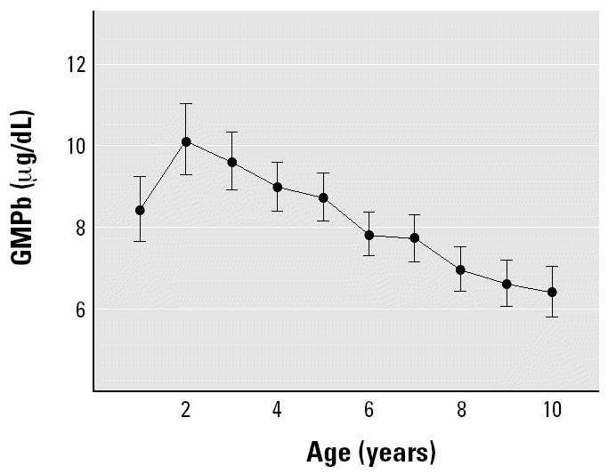
The estimated GMPb of the entire cohort rose from 8.4 μg/dL [95% confidence interval (CI), 7.7 to 9.2] in the first year of life to 10.1 μg/dL (95% CI, 9.3 to 11.0) in the second and decreased thereafter linearly to 6.4 μg/dL (95% CI, 5.8 to 7.1) when children reached their tenth birthday (Figure 3). The GMPb of the cohort at 2 years of age was > 10 μg/dL, a level considered unacceptable in children by the national Mexican and international standards for lead exposure. Blood lead concentration at 2 years and 3 years of age was significantly higher than at 1 year of age (Sidak p ≤ 0.001). Blood lead concentration of the cohort at 9 and 10 years of age fell significantly below the 1-year concentration (Sidak p < 0.01).
Figure 3. Effect of age on estimated GMPb of the entire cohort with 95% CIs.
Children belonging to the lowest and middle SES had 32.3% (95% CI, 17.0 to 49.5) and 9.3% (95% CI, 0.2 to 19.1) higher GMPb than children belonging to the highest stratum (Table 4). In preliminary modeling we failed to find a significant interaction between SES and either age or year of birth on blood lead. Children from families who used ceramic pottery had GMPb levels 18.5% (95% CI, 10.0 to 27.6) higher than did children from families who did not use such pottery (Table 4). Although there was a significant association between ceramic pottery use and poverty (Kruskal–Wallis chi-square = 5.921, df = 1, p = 0.015; 53.8, 38.9, and 31.6% used clay pottery as SES increased from the lowest to the highest stratum), the interaction between poverty and use of ceramic pottery in the prediction of blood lead level was not significant in the multivariate analyses (p = 0.88), and it was not included in the final model. The group of children with complete data had a GMPb 8.6% (95% CI, 1.3 to 15.4) lower than the group with incomplete data (Table 4).
The results showed that the children living in the southwest (residential) and central (mixed commercial–residential) sectors of the city had a GMPb 10.9% (95% CI, 2.4 to 18.6 and 7.2% (95% CI, −2.1 to 15.6) lower than did those who lived in the northeast sector (Table 5). The effect of moving residence during the study was not significant (p = 0.192) in the mixed model and was not included in the above estimations.
Discussion
Design issues.
Our results have at least three limitations. We used only three air monitoring stations to estimate the annual means of atmospheric lead, which were not necessarily representative of the place of residence of all subjects. A better estimate would have resulted from adjusting the children’s air lead exposure according to their place of residence. Because we did not have those data, we selected the station that had the highest atmospheric lead levels (Xalostoc) and the lowest levels (Pedregal) and a station with middle levels (Merced), and we fixed the place of residence of the children based on family residential address into one of the three nonoverlapping zones in which the air monitoring stations were located. Residence in the highest air lead zone (Xalostoc) was significantly associated with higher lifetime blood lead concentrations (p = 0.013) compared with those living in the lowest air lead zone (Pedregal), as had already been found in a prior study in Mexico City (Lara-Flores et al. 1989). We found that 7.5% (n = 24) had changed their address sometime during their participation in the study. We included this information in a preliminary model as a dummy variable and found no significant (p > 0.20) effect. However, we lost contact with 53 subjects before verifying whether their address had changed, and so these data are likely incomplete. Our presented model did not include a term for change of address.
Another limitation of our study is that the use of lead-glazed ceramic pottery was not quantified and was formally assessed only at the start of the study. We asked only whether they used this kind of pottery to serve, cook, or keep foods. For our analysis we used the data provided by the mother during pregnancy. We advised all mothers after application of the pregnancy questionnaire that use of lead-glazed pottery was a risk factor for lead exposure, and we repeated that advice throughout the study. We found that similar data gathered after pregnancy were not very reliable, because mothers admitted “limited use” in the home when home visits were made, despite answering no in previous and subsequent questionnaires, and also revealed that their children would occasionally or frequently eat with family members outside their own home, families that continued to use lead-glazed pottery.
The variable of air lead nested within sub-cohort showed some collinearity with age of subject. Test models (data not shown) without this variable calculated age coefficients and standard errors 1.5–2 times and 1–2 times, respectively, higher than the age coefficients and standard errors calculated with the nested air lead term in the model. Nevertheless, the degree of collinearity was not severe. The pattern of change in the sub-cohort main effect remained unaffected by the addition of the nested air lead variable. Furthermore, the pattern of change in the coefficients of the air lead variable nested with subcohort shows that the strongest relationship of air lead on lifetime blood lead was in the earliest-born subcohort and the weakest in the latest-born subcohort.
Public health implications.
Among the variables tested, atmospheric lead levels were the strongest predictors of blood lead levels of the children across their first 10 years of life. Increased blood lead levels during the second year of life have been reported by several investigators and explained as a consequence of, among other factors, an increase in gastrointestinal capacity to absorb lead, as well as to the characteristic hand-to-mouth activity of this age in which children introduce materials into their mouths, including their generally dirty hands (Baghurst et al. 1992; Rothenberg et al. 1996). This age group has also a greater prevalence of iron deficiency, a factor associated with increased lead absorption and retention (Ruff et al. 1996).
The presence of high blood lead levels among children born in the first 2 years of the study is unlikely to be the result of greater lifetime accumulation of lead in the bones of children born earlier in the study when air lead levels were high, because bone lead is highly labile in infants and young children (O’Flaherty 1995). As shown in Table 4, the coefficients of air lead nested within year of birth fall with later year of birth, reaching essentially zero for the part of the cohort born in 1992. Thus, the higher lifetime blood lead levels of children born in 1987 and 1988 compared with those born in 1991 and 1992 may be most likely caused by the higher air lead concentrations to which the former children were exposed during their lifetime. The model presented here supports the importance of air lead concentration in determining blood lead level throughout the first 10 years of life.
Belonging to a family with low SES significantly contributed to higher blood lead levels at all ages. Other studies have already reported an association among high lead levels and poverty (Carter-Pokras et al. 1990; Lanphear et al. 1998; Mahaffey et al. 1986).
According to the National Nutrition Survey of Mexico of 1999 (Rivera-Domarco et al. 2001), the median of the percentage of consumption of the minimum daily requirement of calcium, iron, and zinc of children 12–59 months of age in Mexico City was 110, 48.6, and 40.7%, respectively. It is possible that frequent and extended conditions of insufficient nutrition in our cohort favored greater digestive absorption as well as a greater retention of lead in the poorer children.
In addition, the poorer residential zones in Mexico City are usually the most industrialized and their pollution is higher. Perhaps children living in those areas have not been favored by the reduction of air lead to the same degree as those with medium SES, because lead emissions from stationary industrial sources were not affected by gasoline lead reduction. However, our models continue to show an effect of poverty even when we account for area of residence. It is clear that we are unable to account for many sources of lead variance in our data set. Some of these unaccounted sources may be partially measured by our poverty index. Nonetheless, the association of SES and lead exposure appears in many investigations from other cultures, each culture likely having its own unique pattern of unmeasured variables that contribute to the effect. After examining the sources specifically addressed in our model as not being responsible for the effect of poverty on blood lead, we found that SES differences in nutrition remain the most plausible explanation of the association.
From a public health viewpoint, the significant effect of the use of clay pots on children’s blood lead levels is important. To this date there have been no effective efforts by authorities to reduce their production, distribution, and use, despite passage of controlling regulations in 1993. Despite the personal counseling that the mothers of our study received about the dangers implied in the use of lead-glazed ceramics, blood lead differences among users and nonusers remain until the end of our study. It is difficult to change behaviors that are considered part of one’s cultural identity, especially when the effects of lead can be nonspecific, subtle, and delayed and can easily be attributed to other causes.
If, in the short term, education by itself has not been enough to obtain a behavioral change in the lead-glazed ceramic users of our cohort, it is important that federal authorities recognize the importance of strict enforcement of existing regulations to eliminate this source of exposure. According to the results of our study, if no children of our cohort had used this type of pottery, there would have been a reduction of 18.8% in the number of blood lead measurements that exceeded the current standard for lead during the study period. We consider that such lead reduction in the Mexican population would potentially have a significant public health impact.
Conclusions
In the last decade, the Mexican government has achieved notable advances in the reduction and control of different lead sources, resulting in a corresponding reduction of blood lead levels of children and adults. Among the adopted measures, the elimination of this metal in gasoline is the one that has had the greatest measurable impact on the reduction of the blood lead levels of the inhabitants of Mexico City. Similar effects have been reported in other countries, where the changeover from leaded to unleaded gasoline has been the major antecedent of sharp declines in average blood lead levels and in the number of children with elevated lead level (Hayes et al. 1994; Luo et al. 2003; Neo et al. 2000; Schuhmacher et al. 1996; Stromberg et al. 1995; Wietlisbach et al. 1995). Since the gradual removal of lead in gasoline started in several countries in the 1970s, nearly 50 nations have already banned lead in gasoline (Landrigan 2002).
In November 1993, the Mexican government established regulations to control the lead content of low-temperature glazed ceramic ware. However, its use is still a very common practice among certain sectors of the Mexican population, with serious implications from a public health viewpoint. It is a problem that is hard to control and eliminate because the clay pots are produced largely by small family enterprises without quality control. Despite the standard to limit the amount of lead that can be released from this kind of earthenware, no official inspection program oversees the production, distribution, and sale of such receptacles. Such lead-glazed vessels can release large amounts of lead into foods and beverages, and today lead-glazed pottery is the principal source of elevated blood lead level in Mexico for populations not exposed to industrial sources.
Several studies have reported that Mexican potters and their families have blood lead levels several times higher than the already elevated levels of the general population (Fernandez et al. 1997; Molina-Ballesteros et al. 1980; Serrato and Olaiz 1996). The beneficiaries of reducing the presence of lead-glazed ceramics would not be limited to just the users but would also include the producers, and an important source of occupational exposure to lead in Mexico would be eradicated.
References
- Albert LA, Badillo F. Environmental lead in Mexico. Rev Environ Contam Toxicol. 1991;117:1–49. doi: 10.1007/978-1-4612-3054-0_1. [DOI] [PubMed] [Google Scholar]
- Baghurst PA, Tong SL, McMichael AJ, Robertson EF, Wigg NR, Vimpani GV. Determinants of blood lead concentrations to age 5 years in a birth cohort study of children living in the lead smelting city of Port Pirie and surrounding areas. Arch Environ Health. 1992;47(3):203–210. doi: 10.1080/00039896.1992.9938350. [DOI] [PubMed] [Google Scholar]
- Bozdogan H. Akaike’s information criterion and recent developments in information complexity. J Math Psychol. 2000;44:62–91. doi: 10.1006/jmps.1999.1277. [DOI] [PubMed] [Google Scholar]
- Carter-Pokras O, Pirkle J, Chavez G, Gunter E. Blood lead levels of 4–11-year-old Mexican American, Puerto Rican, and Cuban children. Public Health Rep. 1990;105(4):388–393. [PMC free article] [PubMed] [Google Scholar]
- Departamento del Distrito Federal 1998. Informe Anual de la Calidad del Aire en el Valle de México—1997. Evaluación del Desempeño Ambiental en Aire. México City:Dirección General de Prevención y Control de la Contaminación.
- Departamento del Distrito Federal 2003. Compendio Estadístico del Sistema de Monitoreo Atmosférico del al Zona Metropoliltana del Valle de México 1986–2002. México City:Dirección General de Prevención y Control de Contaminación.
- Driscoll W, Mushak P, Garfias J, Rothenberg SJ. Reducing lead in gasoline: Mexico’s experience. Environ Sci Technol. 1992;26(9):1702–1705. [Google Scholar]
- Fernandez GO, Martinez RR, Fortul TI, Palazuelos E. High blood lead levels in ceramic folk art workers in Michoacan, Mexico. Arch Environ Health. 1997;52(1):51–55. doi: 10.1080/00039899709603800. [DOI] [PubMed] [Google Scholar]
- Friberg L, Vahter M. Assessment of exposure to lead and cadmium through biological monitoring: results of a UNEP/WHO global study. Environ Res. 1983;30(1):95–128. doi: 10.1016/0013-9351(83)90171-8. [DOI] [PubMed] [Google Scholar]
- Hayes EB, McElvaine MD, Orbach HG, Fernandez AM, Lyne S, Matte TD. Long-term trends in blood lead levels among children in Chicago: relationship to air lead levels. Pediatrics. 1994;93(2):195–200. [PubMed] [Google Scholar]
- Hernandez Avila M, Romieu I, Rios C, Rivero A, Palazuelos E. Lead-glazed ceramics as major determinants of blood lead levels in Mexican women. Environ Health Perspect. 1991;94:117–120. doi: 10.1289/ehp.94-1567967. [DOI] [PMC free article] [PubMed] [Google Scholar]
- Hernandez-Avila M, Gonzalez-Cossio T, Palazuelos E, Romieu I, Aro A, Fishbein E, et al. Dietary and environmental determinants of blood and bone lead levels in lactating postpartum women living in Mexico City. Environ Health Perspect. 1996;104:1076–1082. doi: 10.1289/ehp.961041076. [DOI] [PMC free article] [PubMed] [Google Scholar]
- Landrigan PJ. The worldwide problem of lead in petrol [Editorial] Bull World Health Organ. 2002;80(10):768. [PMC free article] [PubMed] [Google Scholar]
- Lanphear BP, Byrd RS, Auinger P, Schaffer SJ. Community characteristics associated with elevated blood lead levels in children. Pediatrics. 1998;101(2):264–271. doi: 10.1542/peds.101.2.264. [DOI] [PubMed] [Google Scholar]
- Lara-Flores E, Alagon-Cano J, Bobadilla JL, Hernandez-Prado B, Ciscomani-Begona A. Factores asociados a los niveles de plomo en sangre en residents de la Ciudad de México [in Spanish] Salud Publica Mex. 1989;31(5):625–633. [PubMed] [Google Scholar]
- Luo W, Zhang Y, Li H. Children’s blood lead levels after the phasing out of leaded gasoline in Shantou, China. Arch Environ Health. 2003;58(3):184–187. doi: 10.3200/AEOH.58.3.184-187. [DOI] [PubMed] [Google Scholar]
- Mahaffey KR, Gartside PS, Glueck CJ. Blood lead levels and dietary calcium intake in 1- to 11-year-old children: the Second National Health and Nutrition Examination Survey, 1976 to 1980. Pediatrics. 1986;78(2):257–262. [PubMed] [Google Scholar]
- Molina-Ballesteros G, Zuniga-Charles MA, Garcia-de Alba JE, Cardenas-Ortega A, Solis-Camara P. Lead exposure in two pottery handicraft populations. Arch Invest Med (Mex) 1980;11(1):147–154. [PubMed] [Google Scholar]
- Navarrete-Espinosa J, Sanin-Aguirre LH, Escandon-Romero C, Benitez-Martinez G, Olais-Fernandez G, Hernandez-Avila M. Niveles de plomo sanguíneo en madres y recién nacidos derechohabientes del Instituto Mexicano del Seguro Social [in Spanish] Salud Publica Mex. 2000;42(5):391–396. [PubMed] [Google Scholar]
- Neo KS, Goh KT, Sam CT. Blood lead levels of a population group not occupationally exposed to lead in Singapore. Southeast Asian J Trop Med Public Health. 2000;31(2):295–300. [PubMed] [Google Scholar]
- O’Flaherty EJ. Physiologically based models for bone-seeking elements. V. Lead absorption and disposition in childhood. Toxicol Appl Pharmacol. 1995;131(2):297–308. doi: 10.1006/taap.1995.1072. [DOI] [PubMed] [Google Scholar]
- Olaiz G, Fortoul TI, Rojas R, Doyer M, Palazuelos E, Tapia CR. Risk factors for high levels of lead in blood of schoolchildren in Mexico City. Arch Environ Health. 1996;51(2):122–126. doi: 10.1080/00039896.1996.9936004. [DOI] [PubMed] [Google Scholar]
- Rivera-Domarco J, Villalpando-Hernandez S, Gonzalez de Cossio T, Hernandez-Prado B, Sepulveda J. 2001. Encuesta Nacional de Nutrición 1999. Estado Nutricio de Niños y Mujeres en México. Cuernavaca, Morelos, Mexico:Instituto Nacional de Salud Pública.
- Romieu I, Palazuelos E, Hernandez-Avila M, Rios C, Munoz I, Jiménez C, et al. Sources of lead exposure in Mexico City. Environ Health Perspect. 1994;102:384–389. doi: 10.1289/ehp.94102384. [DOI] [PMC free article] [PubMed] [Google Scholar]
- Rothenberg SJ, Karchmer S, Schnaas L, Perroni E, Zea F, Fernandez-Alba J. Changes in serial blood lead levels during pregnancy. Environ Health Perspect. 1994;102:876–880. doi: 10.1289/ehp.94102876. [DOI] [PMC free article] [PubMed] [Google Scholar]
- Rothenberg SJ, Schnaas-Arrieta L, Perez-Guerrero IA, Hernandez-Cervantes R, Martinez-Medina S, Perroni-Hernandez E. Factores relacionados al nivel de plomo en niños de 6 a 30 meses de edad en el Estudio Prospectivo de Plomo en la Ciudad de México [in Spanish] Salud Publica Mex. 1993;35(6):592–598. [PubMed] [Google Scholar]
- Rothenberg SJ, Williams FA, Jr, Delrahim S, Khan F, Kraft M, Lu M, et al. Blood lead levels in children in south central Los Angeles. Arch Environ Health. 1996;51(5):383–388. doi: 10.1080/00039896.1996.9934426. [DOI] [PubMed] [Google Scholar]
- Ruff HA, Markowitz ME, Bijur PE, Rosen JF. Relationships among blood lead levels, iron deficiency, and cognitive development in two-year-old children. Environ Health Perspect. 1996;104:180–185. doi: 10.1289/ehp.96104180. [DOI] [PMC free article] [PubMed] [Google Scholar]
- Schuhmacher M, Belles M, Rico A, Domingo JL, Corbella J. Impact of reduction of lead in gasoline on the blood and hair lead levels in the population of Tarragona Province, Spain, 1990–1995. Sci Total Environ. 1996;184(3):203–209. doi: 10.1016/0048-9697(96)05102-9. [DOI] [PubMed] [Google Scholar]
- Serrato M, Olaiz G. Factores de exposición a plomo en Santa Maria Atzompa, Oaxaca [Exposure factors to lead in Santa Maria Atzompa, Oaxaca] Bol Salud Ambiental, SSA. 1996;6:20–24. [Google Scholar]
- Stromberg U, Schutz A, Skerfving S. Substantial decrease of blood lead in Swedish children, 1978–94, associated with petrol lead. Occup Environ Med. 1995;52(11):764–769. doi: 10.1136/oem.52.11.764. [DOI] [PMC free article] [PubMed] [Google Scholar]
- Wietlisbach V, Rickenbach M, Berode M, Guillemin M. Time trend and determinants of blood lead levels in a Swiss population over a transition period (1984–1993) from leaded to unleaded gasoline use. Environ Res. 1995;68(2):82–90. doi: 10.1006/enrs.1995.1011. [DOI] [PubMed] [Google Scholar]