Three-dimensional, Bayesian image reconstruction from sparse and noisy data sets: Near-infrared fluorescence tomography

Abstract

A method for inverting measurements made on the surfaces of tissues for recovery of interior optical property maps is demonstrated for sparse near-infrared (NIR) fluorescence measurement sets on large tissue-simulating volumes with highly variable signal-to-noise ratio. A Bayesian minimum-variance reconstruction algorithm compensates for the spatial variability in signal-to-noise ratio that must be expected to occur in actual NIR contrast-enhanced diagnostic medical imaging. Image reconstruction is demonstrated by using frequency-domain photon migration measurements on 256-cm³ tissue-mimicking phantoms containing none, one, or two 1-cm³ heterogeneities with 50- to 100-fold greater concentration of Indocyanine Green dye over background levels. The spatial parameter estimate of absorption owing to the dye was reconstructed from only 160 to 296 surface measurements of emission light at 830 nm in response to incident 785-nm excitation light modulated at 100 MHz. Measurement error of acquired fluence at fluorescent emission wavelengths is shown to be highly variable. Convergence and quality of image reconstructions are improved by Bayesian conditioning incorporating (i) experimentally determined measurement error variance, (ii) recursively updated estimates of parameter uncertainty, and (iii) dynamic zonation. The results demonstrate that, to employ NIR fluorescence-enhanced optical imaging for large volumes, reconstruction approaches must account for the large range of signal-to-noise ratio associated with the measurements.

Near-infrared (NIR) diagnostic imaging in tissues can be theoretically extended beyond contrast owing to endogenous chromophores such as melanin, oxy- and deoxy-hemoglobin, fat, and water (1, 2) on introducing NIR-excitable fluorescent contrast agents that can molecularly target and report disease (3, 4). The development of NIR-excitable dyes for diagnostic imaging continues in a number of laboratories (5–7), and numerous groups have demonstrated image reconstruction from synthetic data computed from coupled transport equations describing propagation and generation of excitation and emission light (3). However, although there has been a reported success in fluorescent image reconstruction of a small (9.8-cm³) tissue-like volume from dense continuous wave measurements (8), reports on larger tissue volumes are limited (9). Unlike NIR tomography, which depends on endogenous contrast and involves measurement of reemitted light at the same wavelength as incident light, fluorescence-enhanced optical tomography must address (i) a significantly lower and widely varying signal to noise associated with measurement on large volumes, (ii) sparse data associated with tissue volumes devoid of contrast agent and where no fluorescence is generated, and (iii) incomplete excitation light rejection that corrupts the information content of detected light. These difficulties create unique challenges for the problem of image reconstruction in fluorescence-enhanced optical tomography.

Several approaches have been used to regularize ill-posed inverse problems in optical tomography (for a recent review, see ref. 10). For example, Tikhonov regularization (11) involves a regularization parameter that is added to the diagonal of the matrix to be inverted to achieve diagonal dominance; this parameter is spatially invariant and must be carefully selected to ensure convergence, or can be updated dynamically by using heuristics, as in the Levenberg-Marquardt method (12). Improved results have been demonstrated by using spatially variant regularization based on a priori assumptions of system noise (13), or by using a penalty function based on a priori assumptions on the final parameter distribution (10). Others have used estimates of measurement error based on shot-noise statistics to weight measurements (14). The issue of determining appropriate regularization parameters for arbitrary unknown domains remains a difficult problem. In this contribution, we present the application of a Bayesian reconstruction algorithm, termed APPRIZE (automatic progressive parameter-reducing inverse zonation and estimation), for reconstruction of fluorochrome absorption from experimental measurements through a large three-dimensional (3D) tissue mimicking volume. Unique components of APPRIZE include (i) the minimum-variance (“optimal”) approximate extended Kalman filter (AEKF), which employs both a priori estimates of system noise and on-the-fly calculations of spatially variant measurement error and parameter uncertainty to regularize the inversion and compensate for spatial variability in the signal-to-noise ratio, and (ii) data-driven zonation (DDZ) to stabilize and accelerate convergence and to minimize artifacts. On disabling key features of the algorithm, namely (i) weighting with actual measurement error variances, (ii) damping on the basis of dynamic estimates of parameter uncertainty, or (iii) DDZ, we demonstrate the importance of each of these components of APPRIZE in addressing the challenges of noisy, sparse fluorescence-enhanced frequency domain photon migration (FDPM) measurements for image reconstruction in large tissue volumes.

Materials and Methods

Tissue Phantoms.

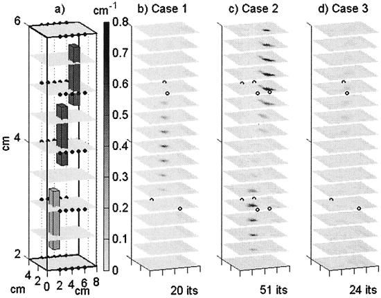
The phantoms each consisted of a 4 × 8 × 8-cm³ open-topped, rectangular, black, opaque acrylic box filled with a solution of 1% Intralipid (Pharmacia and Upjohn) containing 2 × 10⁻⁸ M Indocyanine Green (ICG; Aldrich) as prepared from a 1.1 × 10⁻⁴ M ICG stock solution, to which sodium polyaspartate (Sigma) was added to a concentration of 1.2 × 10⁻⁴ M for dye stabilization (15). Fluorescently tagged heterogeneities consisted of sealed plastic cuvettes containing 1 cm³ of the same Intralipid solution with the exception of a 50- or 100-fold greater concentration of ICG. For the results reported herein, experiments were conducted on a phantom with homogeneous background properties and containing either a single heterogeneity with 100:1 contrast (Case 1, Fig. 1a, center heterogeneity), two heterogeneities, with 50:1 and 100:1 contrast (Case 2, Fig. 1a, bottom and top heterogeneities, respectively), and no tagged heterogeneity (Case 3). Background optical properties, including absorption coefficients at excitation wavelength owing to non-fluorophore (μ_axi) and fluorophore (μ_axf), absorption at emission wavelength owing to non-fluorophore (μ_ami) and fluorophore (μ_amf), and reduced scattering coefficients at excitation (μ′_sx) and emission (μ′_sm) wavelengths, were measured by using FDPM techniques (16) and are shown in Table 1. The reflectance coefficients, required for the computational boundary conditions, were determined (17) to be 0.022 for the acrylic boundaries and 0.431 for the air boundary. Fluorescence lifetime and quantum efficiency of ICG had been previously determined to be 5.6 ns and 0.016, respectively. Integrating absorption owing to fluorophore μ_axf over the 1-cm³ volume of each heterogeneity, the heterogeneity with 50:1 contrast had a true integrated absorption of 0.30 cm², and the heterogeneities with 100:1 contrast each had a true integrated absorption of 0.60 cm².

Figure 1.

(a) The initial homogeneous estimate discretized onto the 9 × 17 × 17 grid used for the initial inversion iteration, and shown with the true locations of the three heterogeneities and the 50 detectors (small dots). (b) Case 1: The reconstructed absorption including the middle fluorescing heterogeneity, interpolated onto the 17 × 33 × 33 grid used for prediction, and shown with the locations of the four sources used (open circles). (c) Case 2: The reconstructed absorption including the top and bottom fluorescing heterogeneities shown with the locations of the eight sources used (open circles). (d) Case 3: The reconstructed absorption of a homogeneous phantom shown with the locations of the four sources used (open circles). Although the phantoms and reconstructions were actually 8 cm in the vertical dimension, only the center 4 vertical cm are shown here.

Table 1.

Background optical properties of tissue mimicking phantoms (in cm⁻¹)

μaxi	μaxf	μsx	μami	μamf	μsm
0.0313	0.006	10.75	0.025	5.06E-04	7.87

FDPM Measurement.

Each 8 × 8-cm² face contained an array of twenty-five 1,000-μm-diameter holes (locations shown in Fig. 1a), fitted with high numerical aperture (n.a. = 0.39) fiber optics (Thorlabs, Newton, NJ; FT-1.0-EMT) and connected to the source and/or detection scheme. For Cases 1 and 3, four sources were used (Fig. 1 b and d), whereas, for Case 2, eight sources were used (Fig. 1c). No collection fiber was closer than 1 cm from another used for collection or source delivery. FDPM measurements were conducted by using the instrumentation previously reported elsewhere (18). Briefly, 785-nm light from a 50-mW laser diode, modulated at 100 MHz, was delivered to each source fiber individually whereas all other fibers collected the light for detection. Two gain-modulated photomultiplier tubes (PMTs; Hamamatsu, Bridgewater, NJ, model R928) fitted with an 830-nm interference filter (CVI Laser, Albuquerque, NM, F10-830) were used as detectors for individual measurements and provided a heterodyned signal at 100 Hz for amplification and data acquisition by using labview (National Instruments, Austin, TX) algorithms written in-house.

The data were sampled at a rate of 10,240 samples per second, with a total of 2,048 samples being collected for a 0.20-s acquisition time for each collection fiber. One PMT provided a “reference” emission signal detected near to the source fiber, whereas the second PMT registered the emission signals of phase-delay (θ), AC amplitude (A), and DC relative to the “reference” PMT. The “referenced” AC fluence at the emission wavelength (Φ_m) was then calculated from the means of AC and phase delay from 100 repeated measurements at each collection fiber, and the measurement error covariance was directly computed from these repetitions of acquired phase and AC. Hence, the error associated with each individual measurement was experimentally acquired, and the measurements were “self-calibrated” without the need for an external calibrating phantom. When the DC values of the collected signals fell below a prescribed set and constant value and the AC no longer provided an adequate emission measurement, the data were not used by the APPRIZE algorithm for image reconstruction. Consequently, the number m of complex emission fluence measurements inverted for Case 1, Case 2, and Case 3 were 172, 296, and 160, respectively.

Image Reconstruction Algorithm.

3D maps of spatially variant absorption owing to fluorophore were estimated by inverting the logarithm of referenced fluence measurements at the emission wavelength by using the APPRIZE algorithm. The APPRIZE method comprises the AEKF (19, 20) combined with DDZ (19), as shown schematically in the following pseudocode and briefly described herein.

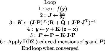where “T” is matrix transpose.

Observable states x are predicted by a forward simulator f based on evolving estimates of uncertain parameters y (step 1). In this work, x refers to the natural logarithm of the complex referenced fluence at the emission wavelength (ln Φ_m), partitioned into its real (ln A) and imaginary (θ) components (and is thus of dimension 2m × 1). The forward simulator f consists of a 3D finite difference model (with n nodes) of the coupled diffusion equations for excitation and emission light propagation with partial current boundary conditions (21), using the current estimate of absorption owing to fluorophore (μ_axf), with all other optical properties set at the values listed in Table 1. Beta-distributed fluorescence absorption, μ_axf was transformed to a normally distributed random variable y (initially, n × 1) through the use of a pseudobeta transform (21), assuming zero to be the minimum feasible absorption whereas the maximum feasible absorption was 0.800 cm⁻¹, with a 0.2 left skew in the distribution. Absorption estimates μ_axf were recovered from updated estimates of y by the inverse pseudobeta transform, and were thereby constrained to fall between zero and 0.800 cm⁻¹. This application of pseudobeta transforms is thus used to constrain both ends of the target parameter distribution in much the same way as logarithmic transforms are commonly used to constrain one end of an estimated parameter distribution to zero, without violating the assumption of least-squares estimators (such as the AEKF) that the estimated parameter y is normally distributed. The feasible range was here deliberately specified to be larger than the true range of absorption (0.006 to 0.598 cm⁻¹), to reduce the likelihood of bias in our results.

The initial stochastic parameterization for each tomographic inversion is highly distributed, to enable high resolution of small heterogeneities. For these experiments, the volume simulating the experimental system was initially discretized into 9 × 17 × 17 nodes (½-cm uniform node spacing) for the inverse problem; these n = 2601 nodes were subsequently merged into fewer zones by using DDZ (step 6). With DDZ, spatially adjacent parameters with similarly updated estimates are identified through cluster analysis and merged into larger stochastic parameter “zones” via random field union (19). Thus, as the estimation proceeds, the number of uncertain parameters decreases dramatically (and all matrices and vectors with initial dimension n are correspondingly reduced), and the size, shape, value, and covariance of the different parameter zones are simultaneously determined in a data-driven fashion. For comparison, reconstructions were also performed without DDZ (step 6 was omitted). Parameter estimates were interpolated back onto a finer mesh (¼-cm uniform node spacing) for the forward solution (step 1) in each iteration.

The Jacobian J (initially, 2m × n) was estimated (step 2) with an approximate adjoint approach (22), with appropriate modifications for the measurement referencing scheme, the use of log measurements, and the use of the pseudobeta transformed parameters. The Jacobian was then used along with the parameter error covariance, P (initially, n × n), the measurement noise covariance R (2m × 2m), and the system noise covariance Q (2m × 2m) to compute the AEKF gain matrix K (initially, n × 2m; step 3), which was then used to update the parameters y (step 4) and parameter error covariance P (step 5). This algorithm is a recursive Bayesian, weighted, damped nonlinear least-squares method, in which the system is regularized by weighting on the inverse of the sum of the measurement error covariance R and system noise covariance matrix Q and by damping on the inverse of the recursively updated parameter error covariance matrix P. Because the Jacobian J is a full matrix, the gain K is also a full matrix. Note that, by conditioning on the logarithm of the complex fluence, the differences between measurements z (2m × 1) and predictions x make the physically meaningful comparisons of phase differences and amplitude ratios. In the experiments reported here, all measurements were used during each iteration. Absorption at the emission wavelength owing to fluorophore (μ_amf) was taken to be the experimentally measured fraction (0.0846) of its absorption at the excitation wavelength (μ_axf); all updates to μ_axf were propagated to μ_amf by this relationship. An adaptive regularization scheme was also put in place to safeguard against overly aggressive updates in highly nonlinear problems, by limiting the step size of updates such that the sum of squared prediction errors (SSE) was never increased by more than 5%. When the relative change in the SSE between predictions and measurements was less than 0.1% and the estimate of μ_axf did not change by more than 0.01 cm⁻¹, the system was said to have converged and the loop was terminated. If the system had not converged within 100 iterations, the reconstruction was aborted.

The Parameter Error Covariance P.

For all inversions, the parameter error covariance P, of the transformed parameter y, was initialized to the identity matrix, corresponding to an initial uncorrelated parameter variance in μ_axf of ≈0.01 cm⁻². Parameter error was assumed to remain uncorrelated for the purposes of locating small fluorescent heterogeneities, thus enabling storage and computation of only the diagonal elements of P. As the information content of an estimate increases and P is correspondingly recursively reduced, the system becomes increasingly damped. For comparison, reconstructions were also performed wherein the update of P (step 5) was omitted.

The Measurement Error Covariance R.

To assess the impact of using the actual measurement error variance and correlation in the weighting scheme, experimental data from the three cases were used to reconstruct images by using (i) the full (spatially correlated) R matrix experimentally obtained; (ii) the diagonal components of R representing the experimentally obtained measurement error variance, with off-diagonal components set to zero; and (iii) the diagonal components of R equivalent to a constant (spatially invariant) measurement error variance computed as the true median of the measurement error variance, with off-diagonal components set to zero.

The System Error Covariance Q.

The system noise covariance Q reflects discrepancies between the computational model and the physical system, including discretization error, round-off error, simplifications in the physics, and errors in parameters considered known. Unlike R, the system noise covariance Q is impossible to determine for physical domains with unknown optical properties, so it was estimated as follows. Measurements (defined as the mean of 100 repetitions) between 200 source/detector pairs in each of six known phantom domains (including zero, one, or two fluorescent heterogeneities with varying levels of contrast and in different locations) were subtracted from simulated measurements generated from computational models of each domain. To generalize these results for use in the AEKF on arbitrary source-detector configurations and arbitrary domains, we determined the median variance of the empirically estimated system noise (median system variance of ln A was 0.1113, and median system variance of θ was 0.0026), and used these as spatially invariant estimates of variance in a strictly diagonal approximation of Q. When both R and Q are diagonal matrices, memory requirements can be reduced by storing only the diagonal elements of these matrices, thereby affording additional potential computational savings.

Summary of Experiments Performed.

In this paper, results of five reconstructions on each of the three phantom domains are presented. (i) “Diagonal R”: The APPRIZE algorithm as described previously was used, incorporating actual (spatially variant) measurement error variance but assuming measurement error was spatially uncorrelated (off-diagonal components set to zero), using recursively updated parameter error covariance P, and applying DDZ. All other experiments varied only one aspect of APPRIZE relative to this implementation. (ii) “Full R” used the full (correlated) measurement error covariance matrix R. (iii) “Median R” used a strictly diagonal R matrix assuming spatially invariant measurement error variance using median values. (iv) “Static P” did not recursively update P (omitted step 5). And (v) “No DDZ” did not apply any data-driven zonation (omitted step 6).

Results

Reconstructions with Diagonal R.

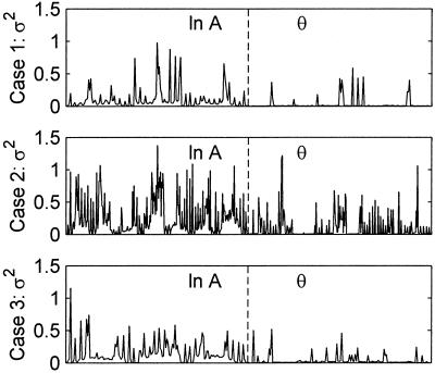
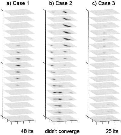
Measurement error variance was determined to be both highly spatially variant and problem specific for the measurements of emission fluence retained for use in each inversion (Fig. 2), but spatial correlation between measurement errors was low. The APPRIZE algorithm used these measurement error variances as the diagonal of the R matrix, thereby ensuring that more accurate measurements were weighted more heavily in determining parameter updates. Starting from an initially homogeneous estimate of μ_axf = 0.006 cm⁻¹ initially distributed over 2,601 parameters (Fig. 1a), the inversions converged for all three phantoms containing zero, one or two fluorescent heterogeneities, with a final reduction of between 50 and 74% (average 59.7%) in the SSEs. DDZ reduced the dimensionality of the parameterization in the final estimates by an order of magnitude from 2,601 to 184, 155, and 270, for Cases 1, 2, and 3, respectively. Because the lengths of the measurement vectors z for the three cases were 344, 592, and 320, all three problems were moved from under- to overdetermined. The three heterogeneities (Cases 1 and 2) were identified in close to their correct locations (Fig. 1 a–c). Defining the volumes of heterogeneities as spatially contiguous voxels with μ_axf > 0.15 cm⁻¹, the integrated value of the lower heterogeneity of Case 2 (0.51 cm²) was less than that of the upper heterogeneity of Case 2 (1.29 cm²), reflecting the different levels of contrast (Fig. 1c), although both were overestimated. The integrated absorption of the single heterogeneity in Case 1 (0.30 cm²) was underestimated, possibly because of the greater source/heterogeneity distances in Case 1 resulting in a lower signal. The highest recovered absorption in the homogeneous Case 3 (Fig. 1d) was only 0.1 cm⁻¹. In the experiments reported here, the adaptive regularization was never invoked on Cases 1 and 3, but did yield a 5% improvement in the SSE for the Case 2 reconstruction. The computation time of the (nonoptimized) implementation of APPRIZE was approximately 10 s per iteration, per source used, on a 950-MHz Pentium III.

Figure 2.

Measurement error variance for each source-detector pair used in the inversions, shown for each of the three test domains. Measurement error variance of the referenced logarithm of AC amplitude is shown in the left half of each panel, and measurement error variance of referenced phase is shown in the right half of each panel.

Reconstructions with Full R.

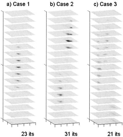
Reconstructions using the full (correlated) measurement error covariance R matrix were also able to resolve the three heterogeneities of Cases 1 and 2, where signal strength at the emission wavelength was relatively high because of the fluorescing heterogeneities (Fig. 3 a and b). Average reductions in SSE were 59.5%, comparable to those obtained with diagonal R. The integrated absorption estimate of the lower heterogeneity of Case 2 (0.31 cm²) was roughly half that of the upper heterogeneity of Case 2 (0.55 cm²), both close to their correct values, although the integrated absorption of the heterogeneity in Case 1 remained underestimated (0.40 cm²). In Case 3 (homogeneous), where signal strength was much lower, using the full R matrix resulted in the appearance of artifacts (Fig. 3c).

Figure 3.

Reconstruction of fluorescence absorption in the three phantom domains by using the full (correlated) measurement error covariance R. Scale and grayscale are as in Fig. 1.

Reconstructions with Median R.

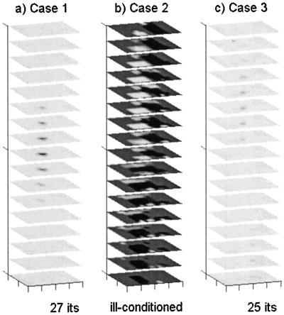
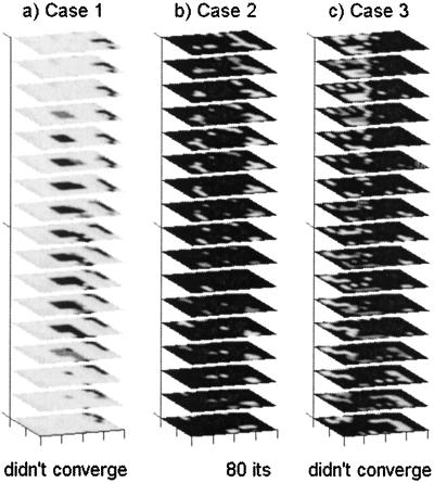
Using diagonal R matrices, where the empirically determined measurement error variances were replaced by spatially invariant median values, resulted in deleterious effects. The Case 2 reconstruction was completely unstable and became ill-conditioned after 33 iterations (Fig. 4b), and an artifact appeared in the Case 3 reconstruction (Fig. 4c).

Figure 4.

Reconstruction of fluorescence absorption in the three phantom domains by using the spatially invariant diagonal measurement error covariance R, using median error variances on the diagonal. Scale and grayscale are as in Fig. 1.

Reconstructions with Static P.

When the recursive update of parameter uncertainty P (step 5) was eliminated, the SSE decreased during the first few iterations for all three cases, but the inversions ultimately became unstable and the reconstructions failed (Fig. 5).

Figure 5.

Reconstruction of fluorescence absorption in the three phantom domains by using static, spatially invariant P as the damping matrix. Scale and grayscale are as in Fig. 1.

Reconstructions with No DDZ.

In these experiments, eliminating DDZ (step 6) actually improved the average reduction of the SSEs slightly, to 63.9%, but artifacts were introduced in the Case 2 and Case 3 reconstructions, and the Case 2 reconstruction still had not converged after 100 iterations (Fig. 6).

Figure 6.

Reconstruction of fluorescence absorption in the three phantom domains without DDZ. Scale and grayscale are as in Fig. 1.

Discussion

Large mixed-determined problems can be inherently ill-posed, leading to problems of non-uniqueness and instability. This ill-posedness is exacerbated by large and variable measurement error, as can be expected of fluorescence measurements through tissues of clinically relevant volumes. APPRIZE incorporates two innovations that address this issue, AEKF and DDZ.

The AEKF is a Bayesian, stochastic, recursive least-squares estimator that can be considered “optimal” in that it minimizes the sum of the estimated parameter error variances, by weighting parameter updates with the inverse of the sum of measurement and system errors, and damping on the inverse of the recursively updated parameter uncertainty. The dynamic and spatially variant regularization is automatic and physically based. The statistical optimality of the AEKF offers potential advantages for nonlinear inverse problems, especially where there is a high degree of scattering and/or nonuniform, sparse or noisy measurements, and precludes the difficult problem of determining how to specify regularization parameters for arbitrary domains. Our results show that the potential benefits of the AEKF innovation are realized with fluorescence-enhanced contrast imaging.

For example, reconstruction of the Case 2 phantom (containing two fluorescently tagged heterogeneities of different contrast levels) failed when not regularized with the actual spatially variant measurement error variance (Fig. 4b). Reconstruction of all three cases failed when the parameter uncertainty P was not dynamically updated (Fig. 5). This observation demonstrates that in the AEKF convergence is achieved even when the initial choice of the damping matrix has not been optimized for convergence. Reconstructions of the Case 3 homogeneous phantom (where measured signal strength was lowest) failed or included artifacts in all reconstructions except the APPRIZE inversion using uncorrelated measurement error variances and parameter uncertainty updating (Fig. 1d).

Although using actual measurement error variances in the regularization proved critical, the importance of modeling correlation between measurement errors is less clear. In these experiments, ignoring low measurement error correlation actually helped to suppress artifacts in the low-signal homogeneous Case 3 domain (Fig. 1d vs. Fig. 3c). Because future improvements in data collection methodologies are expected to reduce measurement error correlation even further, we are optimistic that the computational benefits of using a strictly diagonal R matrix may be exploited in clinical applications involving relevant tissue volumes.

In contrast to Case 2 and 3 reconstructions, inversion of data from the Case 1 phantom (containing one fluorescently tagged heterogeneity) was fairly robust, regardless of how the measurement error covariance was deployed in the conditioning, with reductions of 74% to 79% in the SSE as long as the inversion was damped by the recursively updated parameter error covariance P (Figs. 1b, 3a, 4a, and 6a). This finding underscores the dangers of drawing general conclusions from results on individual domains.

Whereas fluorescent dye distribution in a small (2.5-cm diameter, 9.8 cm³) tissue-like volume has been accurately reconstructed from dense, continuous wave fluorescence measurements by using the simpler algebraic reconstruction technique (8), the results presented herein clearly demonstrate that (i) weighting on spatially variant measurement error variance and (ii) damping with a recursively updated spatially variant estimate of parameter uncertainty can be valuable for inverting sparse, noisy fluorescence measurements in large volumes of highly scattering, tissue-like media. The use of FDPM rather than continuous wave measurement data type will enable application to parameter estimates of fluorescent decay kinetics as a means to perform contrast-enhanced imaging, as afforded by innovative “beacon” dye developments such as by Weissleder and coworkers (7).

The second major innovation of APPRIZE is DDZ. DDZ is used to dynamically reduce the dimensionality of the parameterization, while simultaneously estimating the size and shape of the regions modeled by each parameter zone, thereby moving the problem from underdetermined to overdetermined. DDZ offers several potential benefits over conventional static parameterization, including dynamic increases in computational efficiency, stability, and accuracy of the inversions, and these benefits have been validated by synthetic studies. This study demonstrates that, in experimental fluorescence tomography, DDZ not only enhances convergence, but also tends to suppress background heterogeneity in parameter fields, thereby reducing the number of artifacts, whereas high-contrast fluorescent inclusions remain highly resolved (Fig. 1 vs. Fig. 6).

Summary.

Fully 3D inversion of sparse and noisy experimental FDPM data, in 256-cm³ tissue-mimicking phantoms with a mildly fluorescing background and containing zero, one, or two inclusions tagged with an increased concentration of an NIR excitable fluorophore, was demonstrated. As expected, measurement error variance of fluorescence emission exhibited high spatial variability specific to each domain. Several unique aspects of the APPRIZE inverse method were found to be valuable in the inversions, including regularization with empirically determined measurement error variances and recursively updated parameter uncertainty estimates, and the use of data-driven zonation to dynamically reduce the dimensionality of the parameter space. These results suggest that simultaneous Bayesian estimation and zonation with APPRIZE may be robust and computationally efficient enough for tomographic fluorescence imaging of clinically relevant tissue volumes containing fluorescently tagged inclusions of biological interest, despite the highly variable measurement error expected in such systems. The statistically optimal properties of the APPRIZE inverse method may also prove advantageous for other imaging modalities associated with variable error characteristics.

Abbreviations

APPRIZE

automatic progressive parameter-reducing inverse zonation and estimation

AEKF

approximate extended Kalman filter

NIR

near infrared

FDPM

frequency domain photon migration

DDZ

data-driven zonation

ICG

Indocyanine Green

SSE

sum of squared errors

PMT

photomultiplier tube

3D

three-dimensional

References

- 1.Pogue B W, Poplack S P, McBride T O, Wells W A, Osterman K S, Osterberg U L, Paulsen K D. Radiology. 2001;218:261–266. doi: 10.1148/radiology.218.1.r01ja51261. [DOI] [PubMed] [Google Scholar]
- 2.Shah N, Cerussi A, Eker C, Espinoza J, Bulter J, Fishkin J, Hornung R, Tromberg B. Proc Natl Acad Sci USA. 2001;98:4420–4425. doi: 10.1073/pnas.071511098. [DOI] [PMC free article] [PubMed] [Google Scholar]
- 3.Hawrysz D J, Sevick-Muraca E M. Neoplasia. 2000;2:382–417. doi: 10.1038/sj.neo.7900118. [DOI] [PMC free article] [PubMed] [Google Scholar]
- 4.Ntziachristos V, Chance B. Breast Cancer Res. 2001;3:41–46. doi: 10.1186/bcr269. [DOI] [PMC free article] [PubMed] [Google Scholar]
- 5.Achilefu S, Dorshow R B, Bugaj J E, Rajagopalan R. Invest Rad. 2000;8:479–485. doi: 10.1097/00004424-200008000-00004. [DOI] [PubMed] [Google Scholar]
- 6.Licha K, Hessenius C, Becker A, Henklein P, Bauer M, Wisniewski S, Wiedenman B, Semmler W. Bioconjugate Chem. 2001;12:44–50. doi: 10.1021/bc000040s. [DOI] [PubMed] [Google Scholar]
- 7.Weissleder R, Tung C H, Mahmood U, Bogdanov A., Jr Nat Biotech. 1999;17:375–378. doi: 10.1038/7933. [DOI] [PubMed] [Google Scholar]
- 8.Ntziachristos V, Weissleder R. Opt Lett. 2001;26:893–895. doi: 10.1364/ol.26.000893. [DOI] [PubMed] [Google Scholar]
- 9.Hawrysz D J, Eppstein M J, Lee J, Sevick-Muraca E M. Opt Lett. 2001;26:704–706. doi: 10.1364/ol.26.000704. [DOI] [PubMed] [Google Scholar]
- 10.Hielscher A H, Bartel S. J Biomed Opt. 2001;6:183–192. doi: 10.1117/1.1352753. [DOI] [PubMed] [Google Scholar]
- 11.Tikhonov A, Arsenin V. Solution of Ill-Posed Problems. New York: Wiley; 1977. [Google Scholar]
- 12.Nocedal J, Wright S J. Numerical Optimization. New York: Springer; 1999. [Google Scholar]
- 13.Pogue B W, McBride T O, Prewitt J, Osterberg U L, Paulsen K D. Appl Opt. 1999;38:2950–2961. doi: 10.1364/ao.38.002950. [DOI] [PubMed] [Google Scholar]
- 14.Ye J C, Webb K J, Bouman C A, Millane R P. J Opt Soc Am A. 1999;16:2400–2412. [Google Scholar]
- 15.Rajagopalan R, Utrecht P, Bugaj J E, Achilefu S A, Dorshow R B. Photochem Photobiol. 2000;71:347–350. doi: 10.1562/0031-8655(2000)071<0347:sotota>2.0.co;2. [DOI] [PubMed] [Google Scholar]
- 16.Sevick E M, Chance B, Leigh J, Nioka S, Maris M. Anal Biochem. 1991;195:330–351. doi: 10.1016/0003-2697(91)90339-u. [DOI] [PubMed] [Google Scholar]
- 17.Haskell R C, Svaasand L O, Tsay T-T, Feng T-C, McAdams M S, Tromberg B J. J Opt Soc Am A. 1994;11:2727–2741. doi: 10.1364/josaa.11.002727. [DOI] [PubMed] [Google Scholar]
- 18.Mayer R, Reynolds J S, Sevick-Muraca E M. Appl Opt. 1999;38:4930–4938. doi: 10.1364/ao.38.004930. [DOI] [PubMed] [Google Scholar]
- 19.Eppstein M J, Dougherty D E. Water Resour Res. 1996;32:3321–3336. [Google Scholar]
- 20.Eppstein M J, Dougherty D E. Geophysics. 1998;63:1053–1061. [Google Scholar]
- 21.Eppstein M J, Dougherty D E, Hawrysz D J, Sevick-Muraca E M. IEEE Trans Med Imaging. 2001;20:147–163. doi: 10.1109/42.918467. [DOI] [PubMed] [Google Scholar]
- 22.Lee J, Sevick-Muraca E M. J Biomed Opt. 2001;6:58–67. doi: 10.1117/1.1331561. [DOI] [PubMed] [Google Scholar]