Sympatric speciation by sexual conflict

Abstract

It is well established that sexual conflict can drive an endless coevolutionary chase between the sexes potentially leading to genetic divergence of isolated populations and allopatric speciation. We present a simple mathematical model that shows that sexual conflict over mating rate can result in two other general regimes. First, rather than “running away” from males, females can diversify genetically into separate groups, effectively “trapping” the males in the middle at a state characterized by reduced mating success. Female diversification brings coevolutionary chase to the end. Second, under certain conditions, males respond to female diversification by diversifying themselves. This response results in the formation of reproductively isolated clusters of genotypes that emerge sympatrically.

Sexual conflict occurs when characteristics that enhance the fitness components of one sex reduce the fitness of the other sex. Numerous examples of sexual conflict resulting from the costs of mating, polyspermy, and sensory exploitation have been discussed in detail (1–11). For example, peptides contained in the seminal fluids of Drosophila melanogaster males increase female death rate (3), mating in bed bugs results in severe physical harm to females (9), and if more than one sperm fertilizes an egg, the egg usually dies (11). These detrimental effects of mating on female (or egg) fitness components can be reduced by females evolving resistance to male (or sperm) pre- and postmating manipulations (6). The potential for coevolution because of sexual conflict recently has been evaluated experimentally by using laboratory Drosophila populations (12–14), as well as by using comparative studies of insects (15, 16) and mathematical models (1, 7, 17–20). With respect to speciation, previous discussions have emphasized that sexual conflict drives an endless coevolutionary chase between the sexes and leads to the genetic divergence of isolated populations and allopatric speciation (6, 7, 11, 21, 22). This verbal reasoning has been supported recently by a mathematical model (17) demonstrating that coevolutionary chase between the sexes occurs under a range of conditions. That previous model used a standard Gaussian approximation for the distributions of male and female traits in the population. Here, in contrast, we make no a priori assumptions about the population distributions. By using a simple, explicit genetic model, we show that sexual conflict over mating rate can result in two other general regimes (which could not exist within the realm of the Gaussian approximation). First, rather than evolving away from males, females can diversify genetically and split into separate clusters, effectively “trapping” the males in the middle at a state characterized by low mating success. Second, under certain conditions, males themselves can split into separate groups that subsequently chase different female clusters. As a result, the population becomes subdivided into reproductively isolated groups that emerge sympatrically.

Model

Consider a sexual haploid population with distinct nonoverlapping generations. We concentrate on two possibly linked multiallelic loci: locus x with alleles x_i that are only expressed in females (or eggs), and locus y with alleles y_j that are only expressed in males (or sperm). At the beginning of a generation, the population state is characterized by the frequencies Φ_ij of x_iy_j genotypes. The marginal frequencies of x_i female alleles and y_i male alleles are Φ_f,i = ∑_j Φ_ij and Φ_m,j = ∑_i Φ_ij, respectively. Before mating, males may experience viability selection. Let v_m,j be the viability of y_j males. Then, the frequency of y_j alleles, after viability selection in males, is (v_m,j/v̄_m)Φ_m,j, where v̄_m = ∑_jv_m,jΦ_m,j is the average male viability. We say that two individuals (or gametes) are compatible if mating, fertilization, and offspring development are not prevented by isolating mechanisms. Let Ψ_ij be the probability that female (or egg) carrying an x_i allele is compatible with male (or sperm) carrying a y_j allele. The fraction of males compatible with the female is

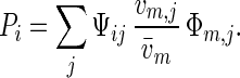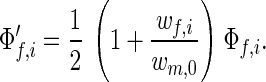
Assume that females are subject to multiple mating attempts but can be fertilized only once. The probability, f_i, that an x_i female (or egg) is successfully fertilized is an increasing function of P_i: f_i = f(P_i). Multiple matings reduce female viability (2–4, 8–10). Ignoring, for simplicity, female interactions with incompatible males, female viability is a decreasing function of P_i: v_f,i = v(P_i). As a result, the overall probability that an x_i female leaves offspring is

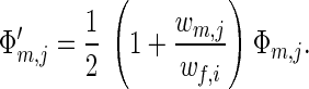
and this is maximized at an optimum proportion of compatible males P_opt, which is smaller than one. In sea urchins, for example, egg fitness is maximized at a level of sperm density which is much smaller than levels common under natural conditions (23). In our model, female mating rate is directly proportional to the proportion of compatible males, and the assumption P_opt < 1 formalizes the idea of sexual conflict over mating rate; for the males, it is optimal to have P_opt = 1, because then all females are susceptible to fertilization by any male. Males that have survived viability selection compete for fertilization opportunities. By the assumptions above, the probability that a y_j male is the one that fertilizes an x_i female is Ψ_ij/P_i. Therefore, the overall probability that a y_j male leaves offspring is

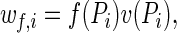
where the two factors in the right-hand side can be interpreted as relative viability and relative mating success. Both female and male overall fitnesses w_f,i and w_m,j are frequency-dependent.

The equations describing the dynamics of genotype frequencies are presented below in Methods. To illustrate the dynamics, the mutation scheme and “preference function” Ψ_ij have to be defined more explicitly. Here, we will use the classical, stepwise mutation model, which was previously used for modeling speciation (24, 25). Specifically, we assume that, at each locus, there is a large number of alleles labeled by integers 0, ∓1, ∓2, …, and that the x_i allele can only mutate to the alleles x_i−1 and x_i+1 and that the y_j allele can only mutate to y_j−1 and y_j+1. For simplicity, we assume that all possible mutations occur with the small but equal probabilities of μ/2. Close matching between parental genes (or traits) is required at all levels of the reproduction process including sperm–egg interaction, mate recognition and mating-pair formation, copulation, and postfertilization development (26–33). To formalize this idea, we posit that Ψ_ij is a symmetric unimodal function of z = i − j: Ψ_ij = Ψ(z) which reaches a maximum value of unity at z = 0. We will also assume that Ψ(z) is convex (d²Ψ(z)/dz² < 0) for small | z |. In our model, genotype frequencies change deterministically. To avoid artifacts of very small numerical values in deterministic models, and also to introduce implicitly the effects of finite population size, each time the frequency of a gamete fell below a small cut-off, Δ, the frequency was set to zero. The inverse of Δ can be thought of as a proxy for the population size.

Methods

Here, we briefly outline some technical details of the analytical methods used for studying the model dynamics. Readers who are not mathematically inclined can safely skip this section.

Our model of sexual conflict is similar to that in refs. 17 and 18. The major difference is that, whereas the latter assumed a normal approximation for male and female trait distributions, our model makes no a priori assumptions about Φ_ij. Note that multimodal distributions presented in some figures could not possibly be described within the realm of the normal approximation. Also, whereas the previous models were phenomenological and postulated specific fitness functions for the sexes, the current model is explicitly genetic and derives these functions from the underlying processes.

Dynamic Equations.

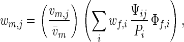
Consider females of x_iy_j genotype and males of x_ky_l genotype. The overall contribution of this pair of genotypes to offspring is proportional to

The term in the parentheses can be interpreted as “fitness” W_ij,kl of the diploid genotype formed by a pair of mating haploids. Simplifying the standard equations for two-locus multiallele diploid systems, one finds that the frequency of x_iy_j genotypes after selection and recombination is

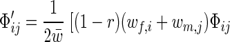where w̄ = ∑_i w_f,iΦ_f,i = ∑_j w_m,jΦ_m,j is the average fitness of the population and r is the recombination rate. Summing over all i or j yields the dynamic equations for allele frequencies:

Effects of mutation on genotype frequencies are described in a standard way.

Invasion Dynamics.

Our approximations are similar to those used within the adaptive dynamics approach (34–36). The major differences are that we do not assume that mutation effects are very small and we allow for an arbitrary number of alleles to be present simultaneously.

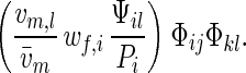
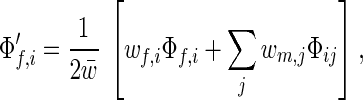
Assume that the population is monomorphic for a female allele x_i. Then Eq. 5b for the frequencies of male alleles simplifies to

This equation is structurally identical to that describing one-locus multiallele haploid systems. Thus, with no mutation, the only male alleles surviving in the population are those maximizing w_m,j. These are alleles maximizing the product v_m,jΨ_i,j with respect to j.

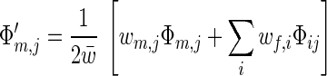
Next, assume that the population is monomorphic for a male allele, say y₀. Then, Eq. 5a for the frequencies of female alleles simplifies to

Thus, with no mutation, the only surviving female alleles are those maximizing w_f,i (and optimizing female mating rate P_i). The absolute maximum of w_f,i is achieved by two alleles x_δ and x_−δ at an optimum number, δ, of mutational steps from y₀. If both of these alleles are present, the population becomes dimorphic.

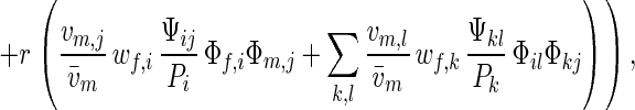
Finally, assume that, initially, the population is monomorphic for male allele y₀ and is dimorphic for two female alleles x_δ and x_−δ that maximize female fitness (2) and are at equal frequencies. This state is an equilibrium of the dynamic system (4). At this state, w̄ = w_f,δ = w_f,−δ and P_δ = P_−δ = Ψ_δ0 = Ψ_−δ0. Eq. 5a simplifies to

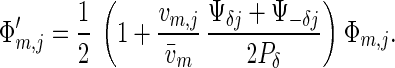This equation immediately shows that the only surviving male alleles are those maximizing the product v_m,j(Ψ_δj + Ψ_−δj). If v_m,1(Ψ_δ1 + Ψ_−δ1) > v_m,0(Ψ_δ0 + Ψ_−δ0)—that is, whether alleles y₁ and y₋₁ have higher fitness than the resident allele y₀—the equilibrium with allele y₀ close to fixation is unstable, and the males will become polymorphic. These results are very insensitive to the precise recombination rate.

Interpretation of Numerical and Analytical Results

Figs. 1–3 illustrate three general regimes observed by iterating the dynamic equations numerically.

Fig 1.

Endless coevolutionary chase between the sexes. Parameters: μ = 10⁻⁵, r = 0.5, Δ = 10⁻⁶, v_m,j = 1, Ψ_ij = exp[−(i − j)²/(2α²)] with α = , and w_f,i = exp[−S(P_i − P_opt)²] with S = 1, P_opt = 0.4. Initial genotype frequencies are Φ₅₆ = 0.99, Φ₅₅ = 0.01. The equilibrium value of P̄ is ≈0.86.

Fig 3.

Sympatric speciation. Parameters are the same as in Fig. 2 except P_opt = 0.4. The equilibrium value of P̄ ≈ 0.42.

Endless Coevolutionary Chase.

In a population with low genetic variation, any male allele that increases male compatibility Ψ_ij with females and any female allele that shifts P_i toward P_opt has a selective advantage (see Methods). This feature can result in a continuous coevolutionary race between the sexes in which females continuously evolve to decrease the mating rate, whereas males continuously evolve to increase it (see Fig. 1). This race was the focus of previous verbal arguments (6, 7, 11, 21, 22) and mathematical models (17, 18). In this regime, there is a dynamic compromise between the sexes, and the proportion of compatible pairs, P̄ = ∑_i P_iΦ_f,i, is intermediate between P_opt and 1. Genetic variation in the population is much higher than expected under mutation–selection balance in a static population (cf. ref. 37).

Buridan's Ass Regime.

In the run described in Fig. 2, the cut-off Δ was reduced, which corresponds to an increased population size, and P_opt was increased, which corresponds to relaxing selection in females. First, a transient period occurred, during which the population evolved to a regime of coevolutionary chase between the sexes (generations 0 through 600). After this, a new female allele, that was substantially different from the resident alleles, successfully invaded the population. The establishment of this allele ended the coevolutionary chase. The population reached an equilibrium at which there are two groups of females (here, at x₃ and x₋₃) both characterized by the values of P_i close to P_opt. Males were trapped in the middle (here, at y₀) and had reduced mating success (Ψ₃₀ = Ψ₋₃₀ = 0.637), a situation resembling the fabled Buridan's Ass. The explanation of this behavior is straightforward. If males are (nearly) monomorphic, say for the y_j allele, then the overall fitness of x_i females depends only on the absolute value | i − j |. Thus, in principle, there are two optimum female alleles, x_j+δ and x_j−δ, which lie at an equal number of mutational steps, δ, from the male y_j allele. Female alleles will split into two clusters if the optimum female alleles are initially present, or if these alleles are produced by mutation. In smaller populations (larger Δ) experiencing stronger selection, the frequency of the second optimum female allele will never exceed the cutoff Δ, and the population will stay in a regime of an endless coevolutionary chase. By contrast, with higher population size (smaller Δ) and weaker selection, mutation produces both optimum female alleles, which then become deterministically established by selection. [Note that if Ψ is a monotonic function of i − j (as used, for example, in ref. 18), then for each male allele, there is a unique optimum female allele, and splitting will not be possible.]

Fig 2.

Buridan's Ass scenario. Parameters are the same as in Fig. 1 except Δ = 10⁻⁸, P_opt = .6 and initial genotype frequencies are Φ₂₃ = 0.99, Φ₂₂ = 0.01. The equilibrium value of P̄ ≈ 0.64.

Sympatric Speciation.

In the run depicted in Fig. 3, the optimum proportion of compatible males P_opt was reduced. By generation ≈1,000, the population reached a state that resembles the Buridan's Ass regime: there are two separate groups of females and a single group of males which are not particularly good at mating with either female group. This state, however, is not an equilibrium. By generation ≈1,200, male alleles split into two groups. This splitting leads to a formation of two large genotypic clusters which start evolving in opposite directions. Also present are two smaller clusters formed by recombinant genotypes. A recombinant female is perfectly compatible with males from one large cluster, whereas a recombinant male with the same genotype is perfectly compatible with females from the other large cluster. The formation of these intermediate recombinant genotypes represents an obstacle to speciation. Nevertheless, genetic divergence of the two clusters leads to substantial reproductive isolation. For example, at generation 2,500, the probability of compatibility between organisms from different clusters is less than one percent. Thus, these clusters can be interpreted as different species which have emerged sympatrically. The regime of coevolutionary chase within-species ends after increasing genetic variation in female alleles leads to the splitting of female alleles into two subclusters within each species. By contrast, genetic variation in male alleles remains very low within each species. Female P_i values are close to P_opt, whereas males get trapped between two female subclusters and have low mating success (the Buridan's Ass regime). For example, at generation 8,000, the most common alleles are x₋₃, y₋₅, and x₋₇ in the first species and x₃, y₅, and x₇ in the second species, the average proportion of compatible pairs is 0.42, and the probability of between-species compatibility is 4%.

The conditions for sympatric speciation can be found analytically. Assume that there is no viability selection in males. (Stabilizing viability selection in males has the general effect of restricting the conditions under which sympatric speciation occurs; see Methods for a general case). Given enough genetic variation, the population first evolves to the Buridan's Ass state where a single male allele, say allele y₀, is close to fixation, and there are two female alleles x_δ and x_−δ at the frequencies close to one half which are at the optimum distance δ from the male allele. Then, if the local convexity condition

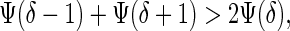applies, male alleles split into two groups, each subsequently evolving toward the closest optimum female allele, resulting in sympatric speciation. If inequality (9) is not satisfied, the population stays at the Buridan's Ass state. Let the function Ψ(z) be sufficiently smooth and have a single inflection point at z*. Then, inequality 9 is satisfied if the second derivative of Ψ(z) at z = δ is positive. This result allows one to express conditions for sympatric speciation in simple graphical terms. Plot two functions: g = Ψ(z) and g = P_opt for positive z. These functions intersect at a point z = δ which gives the optimum “distance” of female alleles from y₀. If δ > z*, condition 9 is satisfied. For example, if Ψ(z) = exp[−z²/(2α²)], then z* = α. Therefore, sympatric speciation takes place if δ > α. If δ < α, the system stays in the Buridan's Ass state.

If P_opt is sufficiently small, the population can undergo further splittings, resulting in sympatric emergence of up to 1/P_opt new species with complex genetic structure (Fig. 4a). Condition 9 also clarifies the reason for our assumption that Ψ(z) is convex for small | z |. If Ψ(z) is concave for all z, then inequality 9 is satisfied for any δ. In this case, male alleles that match existing female alleles can always become established in the population. Consequently, the population reaches a state with more or less continuous genetic variation (see Fig. 4b) rather than with discrete genetic clusters.

Fig 4.

Complex genetic structure. (a) Sympatric emergence of four species. Parameters are the same as in Fig. 3 except P_opt = 0.25 and S = 0.5. P̄ ≈ 0.27. (b) Genetic diversification without distinct cluster formation. Parameters are the same as in Fig. 3, except Ψ_ij = exp[−/(2α²)], P_opt = 0.7, α = 2, and initial genotype frequencies are Φ₁₀ = 0.45, Φ₋₁₀ = 0.55. P̄ ≈ 0.71.

Discussion

Here, we have shown that if there is more than one way for females to reduce the burden of sexual conflict, females can achieve substantially higher fitness by diversifying genetically and splitting into separate clusters than by “running away” in a single pack. Such a diversification (and splitting) will end coevolutionary chase even without direct (stabilizing) selection in one or both sexes. Some data are compatible with the prediction of deceleration of evolution in fertilization proteins (31). The model also predicts complex genetic clustering within populations with female alleles typically having higher variation than male alleles. Although there is some empirical support for both of these predictions (26, 30, 33, 38), more data about levels of genetic variability in compatibility genes (traits) in natural populations are needed.

Sexual conflict generates direct selection on genes responsible for reproductive isolation. This feature makes sexual conflict a very powerful engine of speciation. Here, we were able to find conditions for sympatric speciation analytically. Within the class of preference functions we used, sympatric speciation always happens if the optimum proportion of compatible males P_opt is sufficiently small. The specific form of different functions and parameter values (such as the rates of recombination and mutation, etc.) seem to be of minor importance. Increasing population size will intensify sexual conflict and reduce P_opt. Thus, the periods when local population densities are high will be the most conducive for sympatric speciation and geographic areas of high productivity and, subsequently, of high population densities may be a major source of new species. Subsequent ecological differentiation or some spatial segregation are required for stable coexistence of these species.

Our model is simple enough to allow analysis and yet, we believe, is complex enough to capture the essence of the problem. Its simplicity means it will not directly apply to most metazoans that have much more complex genetic systems underlying mating interactions. However, we expect that the three dynamic regimes identified and studied have a wider applicability than just the original two-locus haploid model. They also can occur in more realistic situations including diploid models, under appropriate conditions. For example, all results obtained for fitness components and the conclusions about conditions of invasion and stabilization of optimal female alleles apply in a diploid version of the original model, with complete dominance. Genetic diversification and speciation are, in our model, driven by strong selection which, in general, is very effective in inducing genetic changes, irrespective of genetic architecture. This is true for morphology, fitness components, or, as in our case, reproductive isolation. These arguments are strongly supported by patterns of selection-driven speciation that have emerged from theoretical studies over the last 40 years. No significant differences have been noted between haploid and diploid models or between models with very small or large numbers of loci (S.G., unpublished work). Stable polymorphism and, ultimately, speciation have been shown to be much more plausible when strong selection directly acts on the loci underlying mating behavior—a feature that also occurs in our model.

In our model, sympatric speciation can occur even when rare genotypes are penalized for being “choosy”, initial genetic variation is very low or absent, and mutation rates are realistically small. In contrast, in recent numerical models of sympatric speciation driven by ecological competition and disruptive natural or sexual selection (34, 35, 39, 40), a choosy female is guaranteed to mate no matter how rare the preferred males are, and initial genetic variation in the loci controlling mating behavior is set at a maximum possible level. The mutation rates used in ref. 34 are higher than those in natural populations by at least two orders of magnitude. These are conditions strongly favoring genetic divergence (and speciation). It is still unclear how these models will fare under more realistic situations. At the same time, simple haploid genetics of reproductive isolation assumed in our model probably simplify conditions for sympatric speciation. Incorporating more complex (e.g., diploid multilocus) genetics into the sexual conflict framework is a necessary next step.

References

- 1.Parker G. A. (1979) in Sexual Selection and Reproductive Competition in Insects, eds. Blum, M. S. & Blum, N. A. (Academic, New York), pp. 123–166.
- 2.Arnqvist G. & Rowe, L. (1995) Proc. R. Soc. London Ser B 261, 123-127. [Google Scholar]
- 3.Chapman T. & Partridge, L. (1996) Proc. R. Soc. London Ser B 263, 755-759. [DOI] [PubMed] [Google Scholar]
- 4.Stockley P. (1997) Trends Ecol. Evol. 12, 154-159. [DOI] [PubMed] [Google Scholar]
- 5.Partridge L. & Hurst, L. D. (1998) Science 281, 2003-2008. [DOI] [PubMed] [Google Scholar]
- 6.Holland B. & Rice, W. R. (1998) Evolution (Lawrence, Kans.) 52, 1-7. [DOI] [PubMed] [Google Scholar]
- 7.Parker G. A. & Partridge, L. (1998) Philos. Trans. R. Soc. London B 353, 261-274. [DOI] [PMC free article] [PubMed] [Google Scholar]
- 8.Civetta A. & Clark, A. G. (2000) Proc. Natl. Acad. Sci. USA 97, 13162-13165. [DOI] [PMC free article] [PubMed] [Google Scholar]
- 9.Stutt A. D. & Siva-Jothy, M. T. (2001) Proc. Natl. Acad. Sci. USA 98, 5683-5687. [DOI] [PMC free article] [PubMed] [Google Scholar]
- 10.Knowles L. L. & Markow, T. A. (2001) Proc. Natl. Acad. Sci. USA 98, 8692-8696. [DOI] [PMC free article] [PubMed] [Google Scholar]
- 11.Howard D. J., Reece, M., Gregory, P. G., Chu, J. & Cain, M. L. (1998) in Endless Forms. Species and Speciation, eds. Howard, D. J. & Berlocher, S. H. (Oxford Univ. Press, New York), pp. 279–288.
- 12.Rice W. R. (1996) Nature (London) 381, 232-234. [DOI] [PubMed] [Google Scholar]
- 13.Holland B. & Rice, W. R. (1999) Proc. Natl. Acad. Sci. USA 96, 5083-5088. [DOI] [PMC free article] [PubMed] [Google Scholar]
- 14.Pitnick S., Brown, W. D. & Miller, G. T. (2001) Proc. R. Soc. London Ser. B 268, 557-563. [DOI] [PMC free article] [PubMed] [Google Scholar]
- 15.Arnqvist G., Edvardsson, M, Friberg, U. & Nilsson, T. (2000) Proc. Natl. Acad. Sci. USA 97, 10460-10464. [DOI] [PMC free article] [PubMed] [Google Scholar]
- 16.Arnqvist G. & Rowe, L. (2002) Nature (London) 415, 787-789. [DOI] [PubMed] [Google Scholar]
- 17.Gavrilets S. (2000) Nature (London) 403, 886-889. [DOI] [PubMed] [Google Scholar]
- 18.Gavrilets S., Arnqvist, G. & Friberg, U. (2001) Proc. R. Soc. London Ser. B 268, 531-539. [DOI] [PMC free article] [PubMed] [Google Scholar]
- 19.Wachtmeister C.-A. & Enquist, M. (2000) Behav. Ecol. 11, 405-410. [Google Scholar]
- 20.Frank S. A. (2000) Evol. Ecol. Res. 2, 613-625. [Google Scholar]
- 21.Rice W. R. (1998) in Endless Forms. Species and Speciation, eds. Howard, D. J. & Berlocher, S. H. (Oxford Univ. Press, New York), pp. 261–270.
- 22.Palumbi S. R. (1998) in Endless Forms. Species and Speciation, eds. Howard, D. J. & Berlocher, S. H. (Oxford Univ. Press, New York), pp. 271–278.
- 23.Franke, E. S., Styan, C. A. & Babcock, R. (2002) Am. Nat., in press. [DOI] [PubMed]
- 24.Nei M., Maruyma, T. & Wu, C.-I. (1983) Genetics 103, 557-579. [DOI] [PMC free article] [PubMed] [Google Scholar]
- 25.Wu C.-I. (1985) Evolution (Lawrence, Kans.) 39, 66-82. [Google Scholar]
- 26.Palumbi S. R. (1999) Proc. Natl. Acad. Sci. USA 96, 12632-12637. [DOI] [PMC free article] [PubMed] [Google Scholar]
- 27.Howard D. J. (1999) Annu. Rev. Ecol. Syst. 30, 109-132. [Google Scholar]
- 28.Tregenza T. & Wedell, N. (2000) Mol. Ecol. 9, 1013-1027. [DOI] [PubMed] [Google Scholar]
- 29.Kubota K. & Sota, T. (1998) Res. Popul. Ecol. 40, 213-222. [Google Scholar]
- 30.Sota T., Kusumoto, F. & Kubota, K. (2000) Biol. J. Linnean Soc. 71, 297-313. [Google Scholar]
- 31.Yang Z. H., Swanson, W. J. & Vacquier, V. D. (2000) Mol. Biol. Evol. 17, 1446-1455. [DOI] [PubMed] [Google Scholar]
- 32.Alipaz J. A., Wu, C.-I. & Karr, T. L. (2001) Proc. R. Soc. London Ser B 268, 789-795. [DOI] [PMC free article] [PubMed] [Google Scholar]
- 33.Swanson W. J., Aquadro, C. F. & Vacquier, V. D. (2001) Mol. Biol. Evol. 18, 376-383. [DOI] [PubMed] [Google Scholar]
- 34.Dieckmann U. & Doebeli, M. (1999) Nature (London) 400, 354-357. [DOI] [PubMed] [Google Scholar]
- 35.van Doorn G. S. & Weissing, F. J. (2001) Selection 2, 17-40. [Google Scholar]
- 36.Metz J. A. J., Geritz, S. A. H., Meszéna, G., Jacobs, F. J. A. & van Heerwaarden, J. S. (1996) in Stochastic and Spatial Structures of Dynamical Systems, eds. van Strien, S. J. & Verduyn Lunel, S. M. (North–Holland, Amsterdam), pp. 183–231.
- 37.Waxman D. & Peck, J. R. (1999) Genetics 153, 1041-1053. [DOI] [PMC free article] [PubMed] [Google Scholar]
- 38.Vacquire V. D. & Moy, G. W. (1997) Developmental Biology 192, 125-135. [DOI] [PubMed] [Google Scholar]
- 39.Kondrashov A. S. & Kondrashov, F. A. (1999) Nature (London) 400, 351-354. [DOI] [PubMed] [Google Scholar]
- 40.Higashi M., Takimoto, G. & Yamamura, N. (1999) Nature (London) 402, 523-526. [DOI] [PubMed] [Google Scholar]