Principal component guided DCGAN for mitigating mode collapse in electromagnetic pulse signal synthesis

Abstract

To mitigate mode collapse in Deep Convolutional Generative Adversarial Networks (DCGANs), this study proposes an innovative deep learning model integrating Principal Component Analysis (PCA)—the PCA-enhanced Deep Convolutional Generative Adversarial Network (PCA-DCGAN)—to mitigate mode collapse during sample generation. By introducing a PCA module prior to the generator, principal components of input samples are extracted and fed into the generator as structured noise input. The resulting components are then fed back into the generator as part of the noise input. This approach breaks from the traditional random selection of generator input noise and provides a more principled direction for optimizing the generator’s parameters. The approach effectively alleviates mode collapse and reduces computational complexity. Experimental results show that the PCA-DCGAN model achieves Fréchet Inception Distance (FID) scores 35.47 and 12.26 lower than those of DCGAN and Wasserstein Generative Adversarial Network with Gradient Penalty (WGAN-GP), respectively. It also significantly improves classification accuracy and reduces loss when training with augmented datasets, thereby validating the effectiveness of the proposed method. The model is applied to generate pantograph-catenary arc electromagnetic interference (EMI) signals, addressing challenges of transient signals and sample scarcity in high-speed railways. This provides an innovative solution for data-scarce domains.

Introduction

In the field of artificial intelligence, data is the core resource driving improvements in model performance^1–3. However, many practical scenarios face challenges such as scarce samples, imbalanced distributions, or high acquisition costs, including difficulties in medical image annotation, few-shot object detection, and capturing specialized physical signals^4,5. To address this issue, data augmentation techniques have emerged, which generate new samples consistent with the original data distribution to effectively expand dataset size and enhance model generalization⁶. Traditional data augmentation methods are mainly divided into two categories: shallow augmentation⁷ based on geometric transformations and advanced augmentation⁸ based on deep generative models. In shallow augmentation methods, geometric transformations (flipping, rotation, cropping) and color transformations⁹ (noise addition, contrast adjustment) generate new samples through simple image operations. For example, Frid-Adar et al. expanded the dataset size to five times the original by random cropping and horizontal flipping in a liver CT image classification task, resulting in a 7% increase in classification accuracy⁴. Lopes et al. combined HSV space color perturbation with random erasing in facial expression recognition, significantly enhancing the robustness of the CNN model⁵. However, these methods generate samples only through low-level feature transformations, making it difficult to capture deep semantic information in complex scenes and limiting sample diversity¹⁰.

With the development of deep learning, deep generative models represented by Generative Adversarial Networks (GANs)⁸ have become the mainstream technology for data augmentation⁹. Specifically, Rashid et al.¹¹ introduced GAN-based synthetic augmentation for skin lesion classification, demonstrating significant performance gains over conventional methods by training a convolutional neural network with GAN-generated dermoscopic images. To address data scarcity challenges in EEG-based neurological disorder classification, Bouallegue et al.¹² developed a Wasserstein GAN (WGAN) to generate synthetic EEG data, significantly improving classification accuracy. In response to train surface anomaly detection challenges caused by scarce abnormal data, Liu et al.¹³ proposed Anomaly-GAN with mask pool, anomaly-aware loss, and local-global discriminators, achieving best FID/LPIPS scores across anomaly categories. Deep generative models generate high-dimensional complex data via latent space mapping, overcoming the limitations of traditional methods^8,14; DCGAN (Deep Convolutional GAN)¹⁵, a classical variant of GANs, demonstrates excellent performance in image generation tasks due to its deep convolutional architecture. However, its generator often suffers from mode collapse during training caused by unstable gradients, resulting in a severe reduction in sample diversity and covering only local modes of the real data distribution^16,17. The root cause of mode collapse lies in the imbalance of the adversarial game between the generator and discriminator: when the discriminator is over-optimized, the generator tends to produce a single “safe sample” to fool the discriminator rather than exploring the entire data distribution¹⁸. To address this problem, researchers^19–21 have proposed three main solutions: (1) Gradient constraint methods stabilize the training process by restricting the discriminator’s gradient range. Among these techniques, WGAN-GP²² introduces a gradient penalty to enforce the discriminator’s Lipschitz continuity, alleviating the vanishing gradient problem; SNGAN²³ applies spectral normalization to constrain the spectral norm of weight matrices, significantly improving sample diversity. Specifically, Zhang et al.²⁴ developed an unsupervised GAN with adaptive-gradient constraints for multi-focus image fusion, addressing boundary blur and detail loss in existing methods. (2) Multi-generator architectures capture different data modes by introducing multiple generators. For instance, Ghosh et al.²⁵ employs a multi-generator competitive mechanism, forcing each generator to specialize in a specific sub-distribution. Hoang et al.²⁶ also introduced a multi-generator GAN framework, which resolves mode collapse by optimizing dual JSD objectives: maximizing inter-generator divergence​and minimizing mixture-to-data divergence, with theoretical guarantees, used a multi-generator architecture in lung nodule detection to generate nodules of varying sizes and shapes, effectively mitigating overfitting in small-sample training. (3) Distribution distance optimization improves distribution similarity metrics to guide the generator in learning global features. As demonstrated by Bellemare et al.²⁷, the Cramer distance is employed as a substitute for the Wasserstein distance in order to mitigate gradient bias; MMD-GAN²⁸ combines maximum mean discrepancy (MMD) with adversarial training to achieve more uniform mode coverage in image generation tasks.

Although the aforementioned methods have made some progress in mitigating mode collapse, the following limitations remain: (1) High computational complexity: gradient penalty and spectral normalization require additional computational resources. For instance, WGAN-GP calculates gradient norms for each input sample during training, resulting in over a 30% increase in training time¹⁷. (2) Limited generator expressiveness: although multi-generator architectures can enhance diversity, the model parameters multiply significantly, and mode overlap among generators often occurs. Li et al.²⁹ pointed out that in multi-generator GAN architectures, gradient conflicts among generators induce training dynamics imbalance, which exacerbates mode collapse and significantly reduces the diversity of generated samples. In SAR image generation using MADGAN, multiple generators may simultaneously focus on dominant modes, exacerbating mode imbalance. (3) Insufficient latent space control: traditional methods rely on random noise as generator input, with no explicit correlation between noise distribution and real data features. For example, DCGAN’s generator input is Gaussian noise, lacking targeted guidance based on principal data components, causing generation to deviate from the effective feature space³⁰.

To address these challenges, researchers have begun exploring new paradigms that combine feature space optimization with guided generator inputs to balance mode diversity and computational efficiency^31–33. Zhang et al.³⁴ introduced a variational autoencoder (VAE) at the generator input to reconstruct latent variables, constraining noise generation direction by encoding real data distribution features; however, this method increases model complexity due to the additional encoder-decoder structure. Zheng et al.³⁵ attempted to decouple generator input features using independent component analysis (ICA), but its capability to model nonlinear relationships is limited. Meanwhile, principal component analysis (PCA), a classical feature dimensionality reduction tool capable of extracting low-dimensional principal components while preserving global statistical properties from high-dimensional data, has been increasingly introduced into generative model optimization. Dou et al.³⁶ proposed PCA-SRGAN, which leverages incremental orthogonal projection to guide a super-resolution GAN for face image reconstruction, effectively improving structural fidelity. However, their approach employed PCA as an auxiliary projection mechanism rather than embedding it into the generator’s latent input. Similarly, Härkönen et al.³⁷ introduced GANSpace, where PCA is applied post-hoc in the latent space of pretrained GANs to discover interpretable control directions for visual editing. While powerful for semantic manipulation, this method analyzes latent directions after training rather than fundamentally addressing the blind randomness of generator inputs.

This paper proposes a deep convolutional generative adversarial network (DCGAN) model incorporating principal component analysis (PCA) as a preprocessing module, termed PCA-DCGAN. The core innovation lies in guiding the generator input with principal component features extracted from real data, rather than relying on purely random noise, thereby providing statistical guidance for parameter updates. Specifically, the PCA module extracts the top k principal components from the training set, constructing a low-dimensional feature space to form semantically enhanced latent variables. Meanwhile, we have also implemented innovative optimizations to the generator and discriminator to further enhance model performance. We introduced rectangular feature maps and a channel balancing strategy to address the common gradient imbalance issues in high-resolution rectangular image generation tasks. This structural optimization approach ensures balanced adversarial competition between the generator and discriminator during training, thereby improving both the quality and stability of generated images. Specifically, we increased the number of transposed convolutional operations in the generator and optimized the design of convolutional kernels, while adopting corresponding convolutional operations and regularization strategies in the discriminator to strengthen its feature extraction capabilities. This approach overcomes the blindness of traditional random noise input, suppresses mode collapse by leveraging intrinsic data features, and simultaneously reduces the computational complexity of the model. Experimental results show that PCA-DCGAN reduces the Fréchet Inception Distance (FID) by 35.47 and 12.26 compared to DCGAN and WGAN-GP respectively, significantly improving the diversity and authenticity of generated samples. Furthermore, this paper applies the model to the generation of electromagnetic interference signals caused by pantograph-catenary arcs.

Pantograph-catenary arcs occur due to instantaneous separation between the catenary and the pantograph, producing electromagnetic signals characterized by strong transience, high acquisition difficulty, and sample scarcity^36,37. Traditional simulation methods rely on physical modeling and struggle to reproduce the true time-frequency characteristics of the signals^38,39. PCA-DCGAN generates electromagnetic interference samples consistent with measured data distributions by analyzing principal component features of existing arc signals, providing high-quality data sources for electromagnetic compatibility testing in rail transit. The contributions of this paper are as follows:

1. A principal component-guided deep convolutional adversarial generation framework (PCA-DCGAN) is proposed, which integrates the PCA module with the generator in an end-to-end manner, exploring a joint optimization of data principal components and generator noise inputs, offering a novel approach to mitigate the blindness of latent space random sampling in traditional GAN models;

2. A generator-discriminator structural optimization method based on rectangular feature maps and channel balancing strategy is proposed, effectively alleviating gradient imbalance issues in high-resolution rectangular image generation tasks;

3. A generation-verification framework for pantograph-catenary arc electromagnetic interference signals is developed, which enhances classification model performance through generated samples, providing a novel data augmentation method for rail transit electromagnetic compatibility testing and preliminarily demonstrating its practical application potential.

Model: PCA-DCGAN

This study introduces the Principal Component Analysis-optimized Deep Convolutional Generative Adversarial Network (PCA-DCGAN), a novel deep learning model designed to address the mode collapse issue frequently encountered during the sample generation process of DCGANs. The overall workflow of the proposed framework is illustrated in Fig. 1. Mode collapse, characterised by the generator producing limited variations of samples that fail to cover the full spectrum of the target distribution, often arises due to gradient instability in the generator. To counteract this, we innovatively integrate a PCA module with the DCGAN generator. Specifically, the PCA module is introduced prior to the generator to extract the principal component features of the sample data. These features are then fed back into the generator’s noise input parameters. This approach breaks away from the conventional random selection of noise inputs for the generator, scientifically guiding the optimisation direction of the generator’s model parameters. By doing so, it effectively mitigates the mode collapse caused by random noise inputs and reduces the computational complexity of the generator model.

Fig. 1.

Overview of research methodology.

Preprocessing

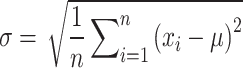
To prepare the data for subsequent model training, we first preprocessed the images by removing coordinate axes and retaining only the essential time-domain and frequency-domain waveforms. All electromagnetic signal images were then uniformly resized to a resolution of 256 × 512 pixels to ensure consistency during PCA processing. Each image was decomposed into three independent color channels—Red (R), Green (G), and Blue (B). The two-dimensional pixel arrays of the three color channels were flattened into one-dimensional vectors to facilitate further processing. To eliminate scale differences in pixel values between different channels and improve the effectiveness of PCA processing, each one-dimensional pixel vector of the color channels was standardized. The standardization steps include:

1. Compute the mean to provide a reference for subsequent standardization

1

where n is the number of elements in each one-dimensional pixel vector, and is the value of the i-th pixel in the vector.

• 2.Compute the standard deviation as an indicator of the data’s dispersion

2

• 3.Standardize the data, so that the processed data has zero mean and unit variance, ensuring each element in the one-dimensional pixel vector becomes a standard pixel value

3

Through the above standardization process, the data of each color channel is transformed into a standard normal distribution with a mean of 0 and a standard deviation of 1, which helps PCA analysis more effectively identify the main directions of variation in the data.

PCA processing

To align the dataset structure with the generator input requirements in the DCGAN framework, a Principal Component Analysis (PCA) module is applied before the generator. This module extracts the principal component features of the image dataset and uses them to construct the input noise vector for the generator, replacing the traditional randomly sampled noise. Specifically, standardized RGB color channel vectors are concatenated to form a composite data matrix. All image samples are aggregated into a batch matrix Z of size , where is the total number of pixels per image, and is the total number of image channels in the batch dataset. The PCA process includes the following steps:

1. Centering: Subtract the mean from each element in the data matrix to eliminate the mean bias in the data

4

where is the element in the i-th row and j-th column of the matrix Z.

• 2.Covariance Matrix Calculation: Compute the covariance matrix of the centered data matrix to reveal the main directions of variation in the data

5

where is the transpose of the data matrix .

• 3.Singular Value Decomposition (SVD): Perform SVD on the covariance matrix to obtain the eigenvalues and eigenvectors, where the eigenvalues represent the variance contribution of each principal component in the data

6

where U is the orthogonal matrix of left singular vectors, is the orthogonal matrix of right singular vectors, and is the diagonal matrix of eigenvalues. The eigenvalues are arranged in descending order, and the image is mainly synthesized by the subspaces corresponding to the larger eigenvalues, which contain more information and explain more of the variance in the data, representing the principal components. The smaller eigenvalues correspond to subspaces with less information, contributing less to the image and representing the subordinate components.

• 4.
  Variance Contribution Rate Calculation: Compute the variance contribution rate of each eigenvalue, i.e., the proportion of the total variance contributed by each eigenvalue. The process continues by progressively discarding smaller eigenvalues until the cumulative variance contribution rate drops below 95%⁴⁰, at which point the number of remaining eigenvalues is determined as the intrinsic feature of the data.

  7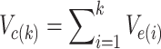

  8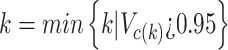

  9

  where is the variance contribution rate, is the i-th eigenvalue, p is the total number of eigenvalues, is the cumulative variance contribution rate, and k is the number of eigenvalues retained, corresponding to the number of principal components.

The intrinsic features of the dataset are effectively extracted through the aforementioned meticulous process, resulting in a feature dimensionality of 15. To augment the model’s capacity for detailed representation while preserving critical data characteristics, the feature dimension is increased by 5 dimensions. This strategic enhancement serves as the optimized input parameters for the DCGAN generator. This approach not only preserves the essential features of the dataset but also enhances the model’s expressive capabilities, thereby establishing a robust foundation for subsequent generative tasks and ensuring the model’s proficiency in capturing and reproducing the nuanced variations inherent in the data. The main steps of PCA decomposition and feature extraction are summarized in Fig. 2.

Fig. 2.

PCA Feature extraction flow.

Optimization of DCGAN structure

In the course of applying DCGAN for data augmentation, it was observed that the original DCGAN architecture predominantly generates low-resolution images with dimensions of 64 × 64 pixels, which results in the loss of many key features inherent in the images. To surmount this limitation, the number of transposed convolutional operations in the generator and convolutional operations in the discriminator was increased, while concurrently optimizing the design of the convolutional kernels. Moreover, given that square images do not correspond to the rectangular shape of the actual images, a rectangular structure was established at the early stage of the generation process to more accurately simulate the shape of real images. Additionally, experimental findings indicated that the discriminator’s relatively faster learning capability compared to the generator in DCGAN frequently induces mode collapse. To attain long-term adversarial balance within the network, the training intensity of the generator must surpass that of the discriminator. Consequently, a balancing strategy was implemented, where the number of channels in each layer of the generator was set to exceed that of the corresponding layers in the discriminator. This strategy enhances the generator’s capacity for feature learning, ensures equilibrium between the generator and discriminator during the adversarial process, and ultimately elevates the quality of the generated images. The detailed structures of the generator and discriminator are depicted in Fig. 3.

Fig. 3.

Internal structure of the generator and discriminator. (Abbreviations: ProjReshape – Projection and Reshape; TConv – Transposed Convolution; BN – Batch Normalization; ReLU – Rectified Linear Unit; Tanh – Hyperbolic Tangent activation; In Img – Input Image; Drop – Dropout; Conv – Convolution; LReLU – Leaky Rectified Linear Unit; Sig – Sigmoid activation.)

Optimization of the generator

The generator receives the input parameters extracted by the PCA module and projects them through a fully connected operation to reshape them into a feature map array with dimensions of 4 × 8 × 1024. Subsequently, five transpose convolution operations are applied, each halving the number of channels sequentially. Each operation is configured with a 2 × 2 convolution kernel and a stride of 2, converting the feature map array into an output array of 256 × 128 × 32.

Batch normalization is introduced after each transpose convolution to improve training speed, stability, and performance⁴¹. Batch normalization normalizes the input data so that the mean of each layer is close to 0 and the standard deviation is close to 1, reducing the impact of internal covariate shift and enhancing the stability of network training. After batch normalization, the ReLU activation function is used to prevent overfitting and improve computational efficiency⁴². The ReLU function introduces nonlinearity by setting negative values to 0 and leaving positive values unchanged, thus enhancing the network’s ability to learn complex data representations and patterns.

Finally, a transpose convolution operation is introduced, configured with three 2 × 2 convolution kernels with a stride of 2, to map the input array to an output array with three channels. The Tanh activation function is applied to map the output data into a compact range, enhancing the richness of sample details and visual quality to generate the image⁴³.

Optimization of the discriminator

The discriminator takes an image of 256 × 512 with 3 channels, matching the output size of the generator, as input. To improve the model’s regularization ability, a dropout operation is introduced after the input layer, randomly dropping 50% of the neurons. Convolution operations are then used for feature extraction, configured with 16 5 × 5 convolution kernels with a stride of 2, converting the input into an output with 128 × 256 × 16 channels. This convolution kernel design provides the discriminator with a broader receptive field, enabling it to capture key features in the image more effectively⁴⁴.

To prevent irregular deformation of the output feature map due to the convolution kernel and stride, the ‘same’ padding strategy is used in the convolution operations to ensure the output feature map dimensions remain consistent. The process continues with four more convolution operations, each using a 5 × 5 convolution kernel with a stride of 2, where the number of convolution kernels doubles at each step. The padding strategy remains ‘same,’ resulting in an output with 8 × 16 × 256 channels. After each convolution operation, batch normalization and the LeakyReLU activation function are introduced. The LeakyReLU activation function, with a small negative slope of 0.2, allows negative values to be partially passed through, helping to improve the discriminator’s expressiveness and enhancing training stability⁴⁵.

Finally, a convolution operation with an 8 × 16 kernel is applied to output a scalar of 1 × 1 × 1. This convolution is necessary to convert the rectangular input into a 1 × 1 output, so an unconventional rectangular convolution kernel is used. The sigmoid activation function is used to limit the output value within the range [0, 1], providing a prediction score that represents the probability of the input image being a real image⁴⁶.

Experiments

Dataset

This study is based on the pantograph-catenary arc electromagnetic signal dataset obtained from the electric field intensity real-train tests conducted on the CRH380B-3747 model train at Changsha EMU Depot in October 2021. The tests covered both in-train and out-train scenarios to capture the electromagnetic interference characteristics of the pantograph-catenary arc in different environments. The test site is shown in Fig. 4, and the main equipment parameters are shown in Table 1. In the inside-the-train tests, the field probe was placed directly beneath the pantograph at the window, with the antenna installed vertically and connected to the optical receiver via fiber optics cables. The optical receiver was then connected to the oscilloscope via a radio frequency coaxial cable. In the outside-the-train tests, the field probe was positioned directly beneath the pantograph, approximately 1.5 m from the edge of the train and 1 m above the ground, with the antenna placed vertically. The antenna was connected to the optical receiver inside the train via fiber optics, and the optical receiver was connected to the oscilloscope through a radio frequency coaxial cable. This setup enabled effective measurement of electromagnetic fields both inside and outside the train.

Fig. 4.

Test scenario of the real-train showing field probe positions (a) inside and (b) outside the train.

Table 1.

Equipment models and parameters.

Name	Model	Parameters
Oscilloscope	Warerunner 8104	Bandwidth: 1 GHz Sampling rate: 20Gs/S
Field probe	WG-EMS-2104	Measuring range: 0.5 V/m-66 V/m Coefficient: 0.05 V/m/mV Bandwidth: 10 kHz-300 MHz

Finally, by applying translation and scaling processing to the measurement results, we constructed a pantograph-catenary arc electromagnetic signal sample dataset, which includes the in-train raising waveform, in-train lowering waveform, out-train raising waveform, and out-train lowering waveform. A total of 230 samples were included, some of which are shown in Fig. 5.

Fig. 5.

Samples of pantograph-catenary arc electromagnetic signal: (a) Pantograph raised(internal field probe); (b) Pantograph raised(external field probe); (c) Pantograph lowered(internal field probe); (d) Pantograph lowered(external field probe).

Model training

In our experiments, a dataset of 200 samples was used for model training after selection. To effectively train the model, the Adam optimizer was chosen, and the relevant parameters for the optimizer were set. Both the generator and the discriminator use the same learning rate of 0.0002 to maintain synchronization during the training process. The gradient decay factor is set to 0.5, and the gradient square decay factor is set to 0.999. These parameters help us dynamically adjust the learning rate to accommodate the model’s needs at different stages of training. A total of 60,000 iterations are performed to optimize both the generator and the discriminator. The mini-batch training method is employed, with each batch processing 10 images. This approach helps the model better capture the intrinsic characteristics of the data while controlling memory usage. The loss functions of the generator and discriminator are used to guide the optimization process. The generator’s loss function focuses on improving the discriminator’s positive evaluation of generated samples, while the discriminator’s loss function aims to enhance its ability to distinguish real samples from generated ones⁴⁷. The expressions of these loss functions are shown below:

10

11

In the equation, z represents the random noise input to the generator, denotes the generated sample after passing through the generator from z, x represents the real sample, and indicates the probability that x is classified as a real sample after passing through the discriminator.

Figure 6 shows the trend of the generator and discriminator loss functions over training iterations in the experiment. The figure reveals the dynamic balance exhibited by the loss functions during the training process. As training progresses, we observe that the generator’s loss function fluctuates more intensely, while the discriminator’s loss function shows reduced fluctuation and gradually stabilizes. This phenomenon can be attributed to the discriminator reaching a relatively stable state in its loss function after learning to distinguish between real and generated images. Meanwhile, in order to continually improve the realism of the generated images, the generator must constantly adapt to the challenges posed by the discriminator, resulting in larger fluctuations in its loss function. Overall, this trend indicates that the generator’s ability to produce high-quality images is gradually improving, while the discriminator’s judgment capability is also increasing. The interaction between the two drives the overall performance improvement of the model.

Fig. 6.

Loss function curves during adversarial training showing (a) generator loss and (b) discriminator loss.

Analysis of generation results

In this section, the experimental results are analyzed from multiple angles to validate the effectiveness of the improvements in the PCA-DCGAN model. Through ablation experiments, we systematically evaluated the impact of the PCA module and the multi-channel structure of the generator on the generation of pantograph-catenary arc electromagnetic signal images. To this end, we selected DCGAN, which can generate high-resolution rectangular images, as the baseline model and gradually introduced improvements on this foundation. We examined the DCGAN model with only the balance strategy and the complete PCA-DCGAN model, which integrates both the balance strategy and the PCA module. Additionally, we introduced the widely used WGAN-GP²² model in the field of image data augmentation as a comparative benchmark. To ensure the fairness and comparability of the experiments, all models were trained for 60,000 iterations, with hyperparameters kept consistent across models except for the input parameters. The input parameters of the complete PCA-DCGAN model were obtained through PCA extraction, while those of the other models were set to the default DCGAN value of 100.The image generation results were analyzed using two evaluation methods: Human Perception Evaluation (HYPE) and Fréchet Inception Distance (FID).

Figure 7 clearly shows the performance differences of each model in the electromagnetic signal image generation task. In terms of visual quality, the images generated by PCA-DCGAN are significantly better than those generated by the other models. Compared to the generation effect of the baseline model with the balance strategy, the addition of the PCA module makes the generated images closer to the original dataset, reducing noise and artifacts in the generated images and improving the richness of image details. Compared to the baseline model’s generation effect, the noise in the generated images is greatly reduced, and the overall naturalness of the images has significantly improved. Although WGAN-GP is widely used and recognized in the industry, its generation effect is not as good as that of PCA-DCGAN in the specific task of this study. The images generated by WGAN-GP have some background noise and have poorer texture compared to the images generated by PCA-DCGAN. This may be due to its higher sensitivity to mode collapse during the training process.

Fig. 7.

Comparison of electromagnetic signal image generation results: (a) Baseline model, (b) Baseline model + balancing strategy, (c) PCA-DCGAN, (d) WGAN-GP.

Early on, Inception Score (IS) was used to quantify the quality of images generated by DCGAN, mainly to measure the consistency of a set of generated images. However, IS fails to directly compare the generated images with real image samples. To address this issue, Martin Heusel and others introduced the more refined FID for evaluation⁴⁸. FID analyzes the feature activations of real and generated images, treats these features as multivariate Gaussian distributions, and calculates their means and covariances to assess the difference in feature distributions between the two sets of images. A decrease in the FID value indicates that the feature distribution of the generated images is closer to that of the real images, which typically means better performance in both quality and diversity of the generated images. Its expression is as follows:

12

In the formula: is the square of the 2-norm, is the trace of the matrix, where and denote the real and generated images, respectively; and represent the means of the features of the real and generated images, respectively; and and are the covariance matrices of the features of the real and generated images, respectively.

A total of 200 images were generated using each method and subsequently compared with the original dataset to calculate the FID score. All FID metrics are averaged over three independent runs to reduce the influence of randomness in GAN training. The results, as detailed in Table 2, are in alignment with our visual analysis, thereby further substantiating the superior performance of PCA-DCGAN in the image generation task. Moreover, the observed differences exceed typical FID fluctuations (< 1–3 points) under consistent evaluation⁴⁹, which further supports the robustness of the reported improvements. It can thus be concluded that the balance training strategy and the PCA module introduced in PCA-DCGAN have exerted a positive and broadly applicable influence on the image generation task. These enhancements have not only optimized the visual performance of the images but also augmented the model’s capacity to capture details.

Table 2.

Comparison of FID values for different methods.

Different methods	FID values
Baseline model	127.09
Baseline model + balancing strategy	122.72
WGAN-GP	103.88
PCA-DCGAN	91.62

Application and verification

To verify the role of PCA-DCGAN in improving the recognition performance of pantograph-catenary arc electromagnetic signal, this study compares recognition tests on the datasets before and after data augmentation. The dataset before data augmentation contains 200 images, while the dataset after augmentation contains 1000 images. The dataset is divided into training and validation sets, with a ratio of 8:2. The recognition model is built based on the PCA-DCGAN discriminator trained with data augmentation. The output section of the discriminator is modified by replacing the LeakyReLU function, convolutional operation, and Sigmoid function with fully connected operation, Softmax function, and classification output function, in order to recognize four types of images: pantograph raised inside the train, pantograph lowered inside the train, pantograph raised outside the train, and pantograph lowered outside the train. The training uses the Adam optimizer, with a learning rate of 0.0002, training for 5 epochs, a mini batch size of 10, and the number of iterations calculated based on Formula 13. The training results are shown in Figs. 8 and 9.

13

Fig. 8.

Comparison of training accuracy (a) before and (b) after data augmentation.

Fig. 9.

Comparison of training losses (a) before and (b) after data augmentation.

As shown in the training accuracy graph in Fig. 8, the recognition model is able to learn a more diverse and sufficient set of samples from the dataset after data augmentation, resulting in higher validation accuracy. The training loss graph in Fig. 9 further confirms this, showing that the dataset after data augmentation results in lower loss function values during training, with the model converging better and achieving more ideal training results on the augmented dataset. This indicates that data augmentation effectively enhances the model’s recognition ability. This result aligns with the theory that data augmentation increases sample diversity and improves the model’s generalization ability.

Conclusion

This paper proposed a PCA-guided DCGAN framework for robust synthesis of pantograph–catenary arc electromagnetic signals. By replacing conventional random noise inputs with principal components extracted from real data, the method anchors the latent space to genuine statistical properties. This design preserves at least 95% of the variance while incorporating a small dimensional expansion to enhance expressiveness. Experimental results demonstrate that PCA-DCGAN improves fidelity and diversity, mitigates mode collapse compared with baseline models, and achieves lower FID scores and higher classification accuracy, confirming its robustness in generative tasks.

Beyond pantograph–catenary arc signals, the proposed framework is general in nature. Since PCA is a statistical decomposition method and DCGAN is a modality-agnostic generative structure, the same integration strategy can be applied to other time–frequency data such as radar spectrograms, electrocardiogram (ECG) waveforms, and Internet of Things (IoT) traffic traces etc. Only minor adjustments to convolution kernel size and hyperparameters are required to suit the properties of different datasets. This highlights the broader adaptability of PCA-DCGAN for signal synthesis tasks across multiple domains.

We also acknowledge that PCA-DCGAN, being built on DCGAN, is relatively less advanced compared with the latest generative architectures. This represents a limitation of the present work. In future research, we plan to extend the proposed PCA-guided latent integration strategy to more powerful models such as StyleGAN, BigGAN, or diffusion frameworks and their derivatives, which will further validate its generality and potentially yield higher-quality synthetic signals. At the same time, we recognize another limitation of the present framework: although it produces statistically meaningful samples for data augmentation, it does not explicitly guarantee the preservation of all physical parameters such as pulse width, rise time, or frequency. Addressing this issue by incorporating domain-specific constraints or direct evaluations of these physical attributes will be an important direction to further enhance the physical interpretability of the generated data while maintaining the advantages demonstrated in the current work.

Author contributions

Zhiwei Gao contributed to conceptualization, project administration, and acted as the corresponding author for coordination and communication. Li Zhao was responsible for writing the original draft, formal analysis, and manuscript organization. Jianhua Zheng and Tao Yi provided funding acquisition and data resources. Chunhui Zhang developed software and implemented programming code. Qingmin Wang performed data validation, manuscript review, and editing. All authors approved the submitted version.

Funding

This work was supported by the Major Scientific and Technological Projects of Universities in Hebei Province under Grant 241130467 A, and the Natural Science Special Project of Hebei Provincial Department of Education (No. CXY2023005).

Data availability

The data that support the findings of this study are available from the corresponding author upon reasonable.

Declarations

Competing interests

The authors declare no competing interests.

References

- 1.Zha, D. et al. Data-centric artificial intelligence: A survey. ACM Comput. Surv.57, 1 (2025). [Google Scholar]
- 2.Janssen, M., Brous, P., Estevez, E., Barbosa, L. S. & Janowski, T. Data governance: Organizing data for trustworthy Artificial Intelligence. Gov. Inf. Q.37, 101493 (2020). [Google Scholar]
- 3.Ntoutsi, E. et al. Bias in data-driven artificial intelligence systems—An introductory survey. Wiley Interdiscip. Rev. Data Min. Knowl. Discov.10, e1356 (2020). [Google Scholar]
- 4.Frid-Adar, M., Klang, E., Amitai, M., Goldberger, J., Greenspan, H. Synthetic data augmentation using GAN for improved liver lesion classification. In: 2018 IEEE 15th international symposium on biomedical imaging (ISBI 2018). 289–293 (IEEE, 2018).
- 5.Lopes, A. T., De Aguiar, E., Oliveira-Santos, T. A facial expression recognition system using convolutional networks. In: 2015 28th SIBGRAPI conference on graphics, patterns and images. 273–280 (IEEE, 2015).
- 6.Van Dyk, D. A. & Meng, X.-L. The art of data augmentation. J. Comput. Graph. Stat.10, 1 (2001). [Google Scholar]
- 7.Krizhevsky, A., Sutskever, I. & Hinton, G. E. Imagenet classification with deep convolutional neural networks. Adv. Neural Inf. Process. Syst. 25, 1097–1105 (2012). [Google Scholar]
- 8.Goodfellow, I. J., Pouget-Abadie, J., Mirza, M. et al. Generative adversarial nets. Adv. Neural Inf. Process. Syst.27, 2672–2680 (2014). [Google Scholar]
- 9.Shorten, C. & Khoshgoftaar, T. M. A survey on image data augmentation for deep learning. J. Big Data6, 1 (2019). [DOI] [PMC free article] [PubMed] [Google Scholar]
- 10.Chen, T., Kornblith, S., Norouzi, M. & Hinton, G. A simple framework for contrastive learning of visual representations. In: International conference on machine learning, PmLR. 1597–1607 (2020).
- 11.Rashid, H., Tanveer, M. A. & Khan, H. A. Skin lesion classification using GAN based data augmentation. In: 2019 41St annual international conference of the IEEE engineering in medicine and biology society (EMBC). 916–919 (IEEE, 2019). [DOI] [PubMed]
- 12.Bouallegue, G. & Djemal, R. EEG data augmentation using Wasserstein GAN. In: 2020 20th international conference on sciences and techniques of automatic control and computer engineering (STA). 40–45 (IEEE, 2020).
- 13.Liu, R. et al. Anomaly-GAN: A data augmentation method for train surface anomaly detection. Expert Syst. Appl.228, 120284 (2023). [Google Scholar]
- 14.Kingma, D. P. & Welling, M. Auto-encoding variational bayes. In: Proc. Int. Conf. Learn. Represent. (ICLR, 2014).
- 15.Radford, A., Metz, L. & Chintala, S. Unsupervised representation learning with deep convolutional generative adversarial networks. In: Proc. Int. Conf. Learn. Represent. (ICLR, 2016).
- 16.Arjovsky, M. & Bottou, L. Towards principled methods for training generative adversarial networks. In: Proc. Int. Conf. Learn. Represent. (ICLR, 2017).
- 17.Mescheder, L., Geiger, A. & Nowozin, S. Which training methods for GANs do actually converge? In: International conference on machine learning. 3481–3490 (PMLR, 2018).
- 18.Arjovsky, M., Chintala, S. & Bottou, L. Wasserstein generative adversarial networks. In: International conference on machine learning. 214–223 (PMLR, 2017).
- 19.Durugkar, I., Gemp, I. & Mahadevan, S. Generative multi-adversarial networks. In: Proc. Int. Conf. Learn. Represent. (ICLR, 2017).
- 20.Mao, Q., Lee, H.-Y., Tseng, H.-Y., Ma, S. & Yang, M.-H. Mode seeking generative adversarial networks for diverse image synthesis. In: Proceedings of the IEEE/CVF conference on computer vision and pattern recognition. 1429–1437 (2019).
- 21.Zhang, H., Goodfellow, I., Metaxas, D. & Odena, A. Self-attention generative adversarial networks. In: International conference on machine learning. 7354–7363 (PMLR, 2019).
- 22.Gulrajani, I., Ahmed, F., Arjovsky, M., Dumoulin, V. & Courville, A. C. Improved training of Wasserstein GANs. Adv. Neural Inf. Process. Syst. 30, 5767–5777 (2017). [Google Scholar]
- 23.Miyato, T. & Koyama, M. cGANs with projection discriminator. In: Proc. Int. Conf. Learn. Represent. (ICLR, 2018).
- 24.Zhang, H., Le, Z., Shao, Z., Xu, H. & Ma, J. MFF-GAN: An unsupervised generative adversarial network with adaptive and gradient joint constraints for multi-focus image fusion. Inf. Fusion66, 40 (2021). [Google Scholar]
- 25.Ghosh, A., Kulharia, V., Namboodiri, V. P., Torr, P. H. & Dokania, P. K. Multi-agent diverse generative adversarial networks. In: Proceedings of the IEEE conference on computer vision and pattern recognition. 8513–8521 (2018).
- 26.Hoang, Q., Nguyen, T. D., Le, T. & Phung, D. MGAN: Training generative adversarial nets with multiple generators. In: International conference on learning representations (2018).
- 27.Bellemare, M. G., Danihelka, I., Dabney, W., Mohamed, S., Lakshminarayanan, B., Hoyer, S. & Munos, R. The Cramer distance as a solution to biased Wasserstein gradients. In: Proc. Int. Conf. Learn. Represent. (ICLR, 2017).
- 28.Li, H., Pan, S. J., Wang, S. & Kot, A. C. Domain generalization with adversarial feature learning. In: Proceedings of the IEEE conference on computer vision and pattern recognition 5400–5409 (2018).
- 29.Li, W., Fan, L., Wang, Z., Ma, C. & Cui, X. Tackling mode collapse in multi-generator GANs with orthogonal vectors. Pattern Recognit.110, 107646 (2021). [Google Scholar]
- 30.Brock, A., Donahue, J. & Simonyan, K. Large scale GAN training for high fidelity natural image synthesis. In: Proc. Int. Conf. Learn. Represent. (ICLR, 2019).
- 31.Karras, T., Laine, S. & Aila, T. A style-based generator architecture for generative adversarial networks. In: Proceedings of the IEEE/CVF conference on computer vision and pattern recognition 4401–4410 (2019). [DOI] [PubMed]
- 32.Esser, P., Rombach, R. & Ommer, B. Taming transformers for high-resolution image synthesis. In: Proceedings of the IEEE/CVF conference on computer vision and pattern recognition 12873–12883 (2021).
- 33.Karras, T. et al. Alias-free generative adversarial networks. Adv. Neural Inf. Process. Syst.34, 852 (2021). [Google Scholar]
- 34.Zhang, H.-D. et al. An effective framework using identification and image reconstruction algorithm for train component defect detection. Appl. Intell.52, 10116 (2022). [Google Scholar]
- 35.Zheng, Y. & Cui, L. Defect detection on new samples with siamese defect-aware attention network. Appl. Intell.53, 4563 (2023). [Google Scholar]
- 36.Dou, H., Chen, C., Hu, X., Liu, Y. & Wang, Z. PCA-SRGAN: Incremental orthogonal projection discrimination for face super-resolution. In: Proc. 28th ACM Int. Conf. Multimedia. 1891–1899 (ACM, 2020).
- 37.Härkönen, E. et al. Ganspace: Discovering interpretable GAN controls. Adv. Neural Inf. Process. Syst.33, 9841 (2020). [Google Scholar]
- 38.Bruni, S., Bucca, G., Carnevale, M., Collina, A. & Facchinetti, A. Pantograph–catenary interaction: Recent achievements and future research challenges. Int. J. Rail Transp.6, 57 (2018). [Google Scholar]
- 39.Wu, G. et al. Pantograph–catenary electrical contact system of high-speed railways: Recent progress, challenges, and outlooks. Railw. Eng. Sci.30, 437 (2022). [Google Scholar]
- 40.Jolliffe, I. T. & Cadima, J. Principal component analysis: a review and recent developments. Philos. Trans. R. Soc. A Math. Phys. Eng. Sci.374, 20150202 (2016). [DOI] [PMC free article] [PubMed] [Google Scholar]
- 41.Li, B. et al. Efficient deep spiking multilayer perceptrons with multiplication-free inference. IEEE Trans. Neural Netw. Learn. Syst.36, 7542 (2024). [DOI] [PubMed] [Google Scholar]
- 42.Monteiro, J., Alves, P., Gomes, A. & Nascimento, S. A colour vision test assisted by neural networks. Acta Ophthalmol.102, e1–e9 (2024).37139848 [Google Scholar]
- 43.Sun, J. et al. Face image-sketch synthesis via generative adversarial fusion. Neural Netw.154, 179 (2022). [DOI] [PubMed] [Google Scholar]
- 44.Wang, W., Li, S. & Jumahong, H. Towards more accurate object detection via encoding reinforcement and multi-channel enhancement. Appl. Intell.55, 1 (2025). [Google Scholar]
- 45.Cai, S. et al. CD-BTMSE: A concept drift detection model based on bidirectional temporal convolutional network and multi-stacking ensemble learning. Knowl.-Based Syst.294, 111681 (2024). [Google Scholar]
- 46.Guo, Q., Wang, C., Xiao, D. & Huang, Q. A novel multi-label pest image classifier using the modified Swin Transformer and soft binary cross entropy loss. Eng. Appl. Artif. Intell.126, 107060 (2023). [Google Scholar]
- 47.Pan, X.-Q., Feng, Z.-Q., Lu, Y. & Zhao, L.-F. LGENER: A lattice-and GAN-based method for Chinese ethnic NER. Alex. Eng. J.115, 297 (2025). [Google Scholar]
- 48.Yan, L. et al. DM-GAN: CNN hybrid vits for training GANs under limited data. Pattern Recognit.156, 110810 (2024). [Google Scholar]
- 49.Chong, M. J. & Forsyth, D. Effectively unbiased FID and inception score and where to find them. In: Proc. IEEE/CVF Conf. Comput. Vis. Pattern Recognit. 6070–6079 (IEEE, 2020).
Associated Data
This section collects any data citations, data availability statements, or supplementary materials included in this article.
Data Availability Statement