Predicting student academic achievement using stacked ensemble learning with deep neural networks and fuzzy-based feature selection

Abstract

Enhancing student performance and academic planning can be greatly impacted by predicting students’ growth. It is possible to customize educational programs to each student’s performance by offering comprehensive insights into their needs and weaknesses. These methods can also aid in recognizing and averting academic issues, which will ultimately improve pupils’ academic performance. In this regard, we have presented a novel method that achieves these goals. The proposed method consists of four basic steps, in the first step, preprocessing of raw data is performed. In the next step, a fuzzy logic-based hybrid model is used to select features related to students’ academic performance. In this method, first, each of the preprocessed features is ranked using Mutual Information (MI) and Analysis of Variance (ANOVA) measures. Then, these rankings are combined with the help of a fuzzy inference model and the features are ranked based on the rules of the fuzzy model. Finally, using the backward elimination feature selection (BEFS) technique, irrelevant features are eliminated and relevant features are selected. In the third step, modeling is performed using three deep neural networks including Convolutional Neural Network (CNN), Long Short-Term Memory (LSTM), and Multilayer Perceptron (MLP), each of which independently tries to model the target variable. In the final step, a meta-model based on the MLP structure is used to extract the target variable based on the predictions from the three deep ensemble models. According to the results obtained through evaluating the model by a questionnaire-based dataset, the proposed methodology achieves significant improvements in predictive accuracy (RMSE 0.6%, MAPE 0.03%), offering a valuable tool for institutions seeking to implement data-driven, individualized academic planning and intervention strategies.

Introduction

Most studies, parents, institutions, and governments throughout the world have been particularly interested in and concerned about students’ academic achievement in school. For an educational institution, it becomes necessary to monitor the academic performance of their students and take respective improvement measures accordingly¹. To achieve the goals and foster an atmosphere of ongoing development, the instructor at an institution of higher learning should assess the performance of the pupils². A number of criteria are used to evaluate an educational institution’s performance. It is expected that the institution improves its ranking based on those factors. In order to attain exceptional performance, schools and universities are interested in providing high-quality instruction. One of the parameters used to rank higher learning institutions is the educational achievement of their students³.

Teachers can learn about the difficulties pupils have in improving their academic performance. To enhance a student’s subpar performance, an educator can upskill them and carry out corrective measures⁴. On the other hand, the quality of instruction at educational institutions is seen as a fundamental element of national development; therefore, it is imperative for these institutions to devise methods that improve their performance systems. Strategies can be formulated following an analysis of student performance, since the advanced estimation of failure rates enables educational institutions to implement preventive measures to mitigate this rate⁵.

The fields in which Artificial Intelligence (AI) and its subfield, Machine Learning (ML), are applied are not restricted to those in which individuals already possess knowledge; rather, they have expanded to include any discipline that offers fresh insights and advancements in various business⁶ or scientific fields^7,8. AI research adds to mankind, science, or AI studies in practically every field of engineering, social, and medical science, much as the large and little bricks used to make a structure. As this construction remains incomplete, there has been an upsurge in interest in AI studies in educational sciences in recent years⁹.

Although ML methods have been widely used in recent years, one of the challenges is that a single model cannot accurately and comprehensively analyse the characteristics related to students’ academic performance and thus provide accurate predictions. To address this deficiency, we use ensemble techniques to cover the limitations of individual models and increase the accuracy of predictions. The innovation of our research consists of two main aspects. The first innovation is the use of a new feature selection system that has not been used in previous research to predict students’ academic performance. In this system, the scores calculated for feature ranking using MI and ANOVA criteria are combined, and then a fuzzy model is used to finally rank the features based on these two criteria. The second innovation is the proposed ensemble structure that supports a stack structure. This structure includes a meta-learner that is used to ensemble the outputs of deep neural networks to predict the impact of students’ performance.

This approach significantly increases the prediction accuracy and helps to identify important components in students’ academic performance. The paper’s contributions are as follows:

• Presenting a feature selection system based on the combination of MI and ANOVA that effectively predicts students’ academic performance.

• Utilizing a fuzzy model that ranks feature based on MI and ANOVA, contributing to the improvement of prediction accuracy.

• Offering a proposed ensemble structure that employs a meta-learner to ensemble the outputs of deep neural networks and aims to identify important components in students’ academic performance.

The paper continues in this manner: studies similar to the current one is discussed in “Related work”. “Research methodology” describes the proposed approach, while “Research finding” provides the study’s findings and “Conclusion” summarizes the conclusions.

Related work

This section reviews the previous work done on predicting student academic achievement. Further, this review also extends the analysis to various methods and techniques used in the past research for identification of factors affecting academic performance. This review will help in the identification of strengths and weaknesses of the existing methods to improve the accuracy of prediction and improvement in student academic outcomes.

Batool et al.¹⁰ compared 260 studies related to educational data mining, conducted over a period of 20 years, with a view to finding the factors that influence the predictions and the techniques of data mining in use. The results pointed out ANN and Random Forest among commonly used techniques, whereas WEKA was found to emerge as one of the trending tools in the field.

Hussain and Khan¹¹ assessed the BISEP-Peshawar dataset, the quality of education, and its sustainability goals. After preprocessing, training of the regression model, and a decision tree classifier, the results depicted that the ML technology has effectively predicted the student performance.

Mallak et al.¹² predicted the academic performance of E-Commerce students at Palestine Technical University-Kadoorie using a Markov chains model and a decision tree algorithm, which resulted in an accuracy of 41.67%, showing efficiency and generalization.

Issah et al.¹³, in their review, conducted a systematic literature review and highlighted the role of ML in performance traits analysis in academic institutions. The review also pointed out that academic and demographic attributes are most influential, although it also presented some gaps in research regarding basic academic performance and intervention plans.

Pallathadka et al.¹⁴ utilized data mining approaches to forecast student success in a course, employing ML methods including Naive Bayes and Support Vector Machine (SVM), while examining the UCI ML dataset.

Nurudeen et al.¹⁵ introduced a model of social media influence factors that evaluated the effect of social media on student academic performance, demonstrating a substantial negative correlation between social media influence factor (SMIF) variables and student GPA. This model explained 30.7% of the variability and exhibited a predictive accuracy of 55.4%.

Arizmendi et al.¹⁶ explored the use of Learning Management System (LMS) digital data in higher education for predicting student success. They discussed its potential for intervention design, ethical issues, and ML algorithms, concluding with an empirical example.

He et al.¹⁷ investigated the effectiveness of project-based learning on developing student science proficiency. They found that students’ post-unit assessments were predictive of their summative science achievement as measured by a third-party-designed test aligned with US science standards.

Acosta-Gonzaga¹⁸ conducted a study including 243 university students, revealing that self-esteem and motivation greatly influence academic engagement, while metacognitive engagement predicts academic performance. The research highlighted the necessity of metacognitive methods.

Abid et al.¹⁹ indicated a significant positive correlation among the reading habits, study skills, and English achievement of secondary school students in Punjab of Pakistan. This study also depicted the moderate positive association among these constructs. It also recommended that teachers should plan assignments for reflective thinking.

Murnawan et al.²⁰ explored sustainable educational data mining from 2017 to 2022 and found that common predictors for student academic performance were demographic, grades, social factors, and online learning activities.

Beckham et al.²¹ applied Pearson’s correlation in the study of factors influencing students’ performance. Past failures had negative influences on grades, but the mother’s schooling positively influenced grades. Prediction models were then made using ML. Of these, the best model was MLP 12 neuron.

Liu et al.²² employed a feedforward spike neural network to improve the accuracy of student performance prediction to 70.8%, which improves targeted management, an effective learning supervision plan, further improving teaching quality and student outcomes.

Mohd Zaki et al.²³ conducted a study with 1,052 students from the UiTM Pahang Branch, revealing that demographic characteristics included gender, family income, area, and national secondary school assessment findings were predictors of academic accomplishment.

Chukwu et al.²⁴ assessed the efficacy of a ML expert system at the Federal Polytechnic Bida to predict student academic performance using Python programming and fuzzy logic algorithms, but requiring administrator logins.

Yau et al.²⁵ performed a study at the Federal University Birnin Kebbi utilizing ML to forecast the influence of mobile phone usage on students’ academic performance. Decision Tree and Random Forest models were utilized, with the Decision Tree attaining 57% accuracy and the Random Forest getting 63% accuracy.

Furthermore, advanced feature selection techniques and hybrid machine learning models are increasingly applied across domains to improve predictive performance and model efficiency. Various complex methods are demonstrated in reviewed literature. For instance, studies in biomedical classification have employed fuzzy logic²⁶ and multi-phase hybrid methods combining soft computing and feature extraction²⁷ for selecting relevant genes from high-dimensional data. A different set of researchers employed optimization-based algorithms derived from game theory which include kernel SHAP^28,29 to optimize feature selection for classification tasks. These works demonstrate effectiveness but concentrate on classification problems which exist outside the educational field. The research field has investigated hybrid approaches which use GA-based selection for clustering categorical data³⁰.

It is important to note that the methodology of the given study contrasts with the methodology of longitudinal or time-series-based approaches that are another significant direction of educational data mining. Longitudinal analyses are concerned with modelling the performance of students over time, and may involve such methods as time-series regression to represent patterns and temporal correlations in learning curves³¹. These techniques are priceless in the realization of student development and facilitating interventions in the course of a long-term academic program. On the other side, the current research uses a cross-sectional design. We aim at making a strong prediction of the final academic performance of a student based on a detailed profile of his/her demographic, social, and personal characteristics taken at one point in time. Thus, our literature review is reasonable to concentrate on the works that, similarly to our research, utilize machine learning to make predictions in relation to similar static and feature-rich data.

Our research concentrates on predicting continuous student academic achievement which represents a regression task within educational domains. The proposed method merges statistical (ANOVA) and information-theoretic (MI) ranking with Mamdani fuzzy inference and backward elimination (BEFS) to create a unique solution for this prediction task. The particular feature selection method succeeds in identifying academic features that impact continuous performance assessment. The proposed framework integrates a deep ensemble stacking structure that includes CNN, LSTM and MLP base models and an MLP meta-model. The integrated method which merges our suggested fuzzy-based hybrid feature selection solution with deep ensemble stacking for continuous academic grade prediction makes our work stand apart from current research by providing an extensive specialized solution to boost educational data mining predictive accuracy.

Research methodology

In this section, the method of collecting the necessary data for the research and the characteristics of this data are described. Then, the steps of the proposed method for predicting the academic performance of students in higher education are presented.

Data

In this research, the information used was collected through the distribution of questionnaires among students at universities in Nanjing, China. This dataset includes information from 628 students from two faculties of engineering (Computer Science, Electrical and Electronic Engineering). During the distribution of the questionnaires, the academic and educational conditions of the students at the beginning of their studies were collected, and then the average grades of each responding student at the end of the academic term were recorded as the target variable. Among these data, 383 records belong to female students, while the remaining samples pertain to male students. The age range of the responding population is 20 to 31 years, with an average age of 23.78 years. Table 1 includes the list of information available in the database.

Table 1.

Database specifications.

Identifier	Title	Type
I1	Study Location	Nominal Discrete
I2	Sexuality	Nominal Discrete
I3	Age (in years)	Continuous Numeric
I4	Status of Residential	Nominal Discrete
I5	Family Individuals	Discrete Numeric
I6	State of Parents’ Living (Divorce Status)	Nominal Discrete
I7	Level of Education (Mother)	Ordinal Nominal
I8	Level of Education (Father)	Ordinal Nominal
I9	State of Employment for Mother	Nominal Discrete
I10	State of Employment for Father	Nominal Discrete
I11	Justification for Selecting the Study Location	Nominal Discrete
I12	Guardian of the Student	Nominal Discrete
I13	Time Distance from Residence to Place of Study	Continuous Numeric
I14	Duration of Study per Week	Continuous Numeric
I15	Average of the obtained Grades in the Last Semester	Continuous Numeric
I16	Receiving a Scholarship	Nominal Discrete
I17	Receiving Funding Assistance from Parents	Nominal Discrete
I18	Attendance at Extra Classes	Nominal Discrete
I19	Taking Part in Other Extracurricular Events	Nominal Discrete
I20	History of Scientific Contest Attendance	Nominal Discrete
I21	Willingness for Continued Education	Nominal Discrete
I22	Access to Internet at Home	Nominal Discrete
I23	Status of Emotional Relationships	Nominal Discrete
I24	Relationship Quality with Family Members	Ordinal Nominal
I25	After Classes, Idle Time	Continuous Numeric
I26	Communication with Fellow Students Outside of the Place of Study	Nominal Discrete
I27	Drinking Alcohol Throughout the Workweek	Nominal Discrete
I28	Drinking Alcohol Throughout the Weekends	Nominal Discrete
I29	Present Health State	Ordinal Nominal
I30	Days being Absent in Classes	Continuous Numeric
-	Average Final Grades of the Student	Continuous Numeric

All participants were adult university students and provided written informed consent prior to their participation. The research was conducted in accordance with the ethical guidelines of the researchers’ institution in Nanjing, China, and the principles outlined in the Declaration of Helsinki and the ethical principles of the Belmont Report. The study protocol, involving an anonymized questionnaire focused on educational background, lifestyle factors, and academic information, was determined to pose minimal risk to participants. The data collected (see Table 1) did not include invasive procedures or the collection of highly sensitive personal identifiers that could lead to harm or discrimination, and all data were fully anonymized prior to analysis to ensure participant privacy and confidentiality. Ethical review and approval were waived for this study by the School of Education of Renmin University of China, as the research involved anonymized data and was deemed minimal risk according to institutional guidelines.

According to Table 1, the collected dataset consists of 30 independent features that describe students’ educational background and lifestyle; the dependent variable represents the average final grades of the student, reflecting their academic achievements. For example, the feature “age” is presented as a natural number measured in years. Characteristics such as “travel time from home to place of study,” “study duration per week,” and “free time after classes” are described numerically and measured in minutes.

The residence status indicates whether the student uses a dormitory, lives independently, or resides with parents. Additionally, the characteristic regarding the education level of parents can take one of the following values: 1 - Illiterate, 2 - Diploma, 3 - Bachelor’s, 4 - Master’s, and 5 - Doctorate or higher. The employment status of parents has one of the following conditions: 1 - Education, 2 - Healthcare, 3 - Services, 4 - Legal, 5 - Government, and 6 - Other. The reason for choosing the place of study can be one of the following: 1 - Personal Interest, 2 - Proximity to Residence, 3 - Cost, and 4 - Other. Furthermore, the legal guardian can be categorized as one of the following: 1 - Parents, 2 - Other. These characteristics are presented either numerically or as ranked values. In addition, other nominal characteristics in the database are represented as logical features with values of true or false. The target parameter in this dataset is the average final grades of the student, described as a numerical value between 0 and 20.

Proposed method

The multi-step and comprehensive approach in this research is proposed to enhance the accuracy and validity of the prediction model of student academic success. This is an approach that contains four important steps:

1. Pre-processing of raw data.

2. Feature selection based on fuzzy logic.

3. Deep neural network-based modelling.

4. Prediction based on ensemble stacking.

Figure 1 illustrates the mechanism of the proposed strategy for predicting student performance as a diagram. During this pre-processing, the raw data is prepared for further steps involved in the proposed model through various techniques. The qualitative features start getting converted to quantitative features during this process so that these features can be utilized by different ML models. The management of the missing values is the second process in this pre-processing step, which is conducted through the K-Nearest Neighbour (KNN) strategy. This avoids the effect of incomplete data causing deterioration in model performance. Data normalization happens at the end of pre-processing; it helps reduce the effect of different feature scales on model performance.

Fig. 1.

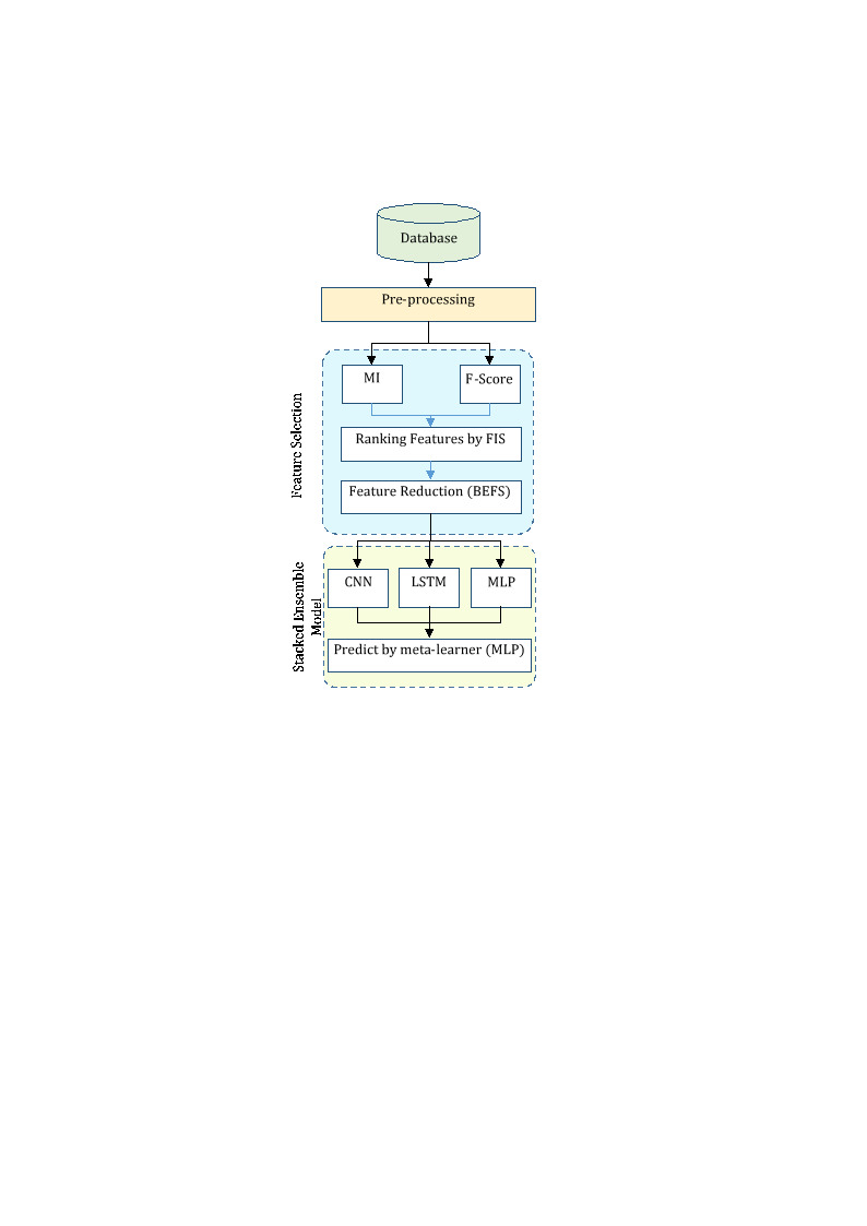
Steps of the proposed method for predicting student performance.

In the feature selection step, approaches such as MI and the F-statistic in one-way ANOVA are firstly adopted to weight features, then fuzzy logic is used to rank feature importance based on the determined weight values. Because fuzzy logic can model vague and uncertain information, it is especially fit for selecting important features from the training data. Along with this, the BEFS algorithm removes insignificant features step by step. This removes redundant features of a model and gives better accuracy for it.

In the third step of the proposed method, three types of deep neural networks are employed to model student performance based on the selected characteristics describing them. This hybrid model combines three distinct deep neural networks: CNN, LSTM, and MLP. While CNN models are very good at the extraction of local features from data, LSTM networks are designed to model time sequences and consider temporal dependencies within the data. In contrast, MLP is especially powerful for learning complex and nonlinear patterns in data. These three neural network variants have been selected for their capability of learning complex features and modelling nonlinear relationships in the training data.

Finally, in the last step of the suggested method, a stacked ensemble learning technique is utilized to calculate the system’s final output, improving the model’s accuracy and stability. This technique helps reduce the error associated with each of the models by combining the outputs of the deep neural networks from the third step, leading to an improvement in the overall model performance. This stacked ensemble system utilizes an MLP to model the relationship between the outputs obtained in the third step and the target variable. The learning neural network improves model accuracy by learning the optimal weights to combine the outputs of the base models.

Pre-processing

The preparation of raw data through preprocessing is the first step of the proposed method, which aims to convert the data format described in Sects. 3 − 1 into a structure interpretable by ML models through three sub-processes. These processes are:

• (A)Feature transformation.

  The transformation process of feature targets nominal and ordinal data and translates them into numerical values. During this processing, discrete nominal features are transformed into numeric vectors based on the frequency of values. Firstly, for each feature, a frequency vector of unique values is created and those unique values are sorted in an ascending manner based on their frequency. Each unique value is then replaced with its corresponding numeric identifier in the sorted list. Thus, for each discrete nominal feature, the values with the lowest frequency are assigned the number 1, and other values receive a numeric value proportional to their frequency. However, ordinal nominal features depend on the rank of their unique values for transformation. In other words, unique values of ordinal features are sorted in an ascending manner by their rank and each nominal value will be replaced by a corresponding number with respect to its rank in order to turn the database into a numerical matrix.

• (B)Management of missing values.

  Proper management of missing values in the data is a critical step in the data preparation process. The choice of appropriate methods for handling missing values depends on the type of data, the extent of missing data, and the goals of the analysis. By selecting and implementing the appropriate method, the negative impacts of missing values on the results of ML models can be avoided, leading to more accurate and reliable results. One effective method for replacing missing values in the data is the KNN algorithm. In this method, for each data sample with a missing value KNN in the feature space are identified. Then, the missing feature value in the sample of interest is replaced with the mean or median of that feature’s values in the KNN. The KNN algorithm works well for imputation of missing values in numeric features. It is based on the principle of similarity, that the closer two samples are to each other in feature space, the closer their attributes are.

  Using KNN, it is possible to fill missing values according to the pattern present in the data and the relationship between the samples. The proposed method employs an empirical approach to set the K value of the KNN model at 5. A K value of 5 was selected for this study through empirical testing to achieve the best performance for our particular dataset. The imputation accuracy was tested through preliminary experiments which evaluated values. The experiments used artificial value removal to test KNN configurations for their ability to make accurate imputations. A comparison between KNN imputation and basic imputation methods using mean and median strategies was conducted. The precision with which local information was captured, combined with processing speed was most favorable using K=5. The experimental findings confirmed K = 5 as the optimal choice for missing value handling in the dataset because it performed better than other K values and basic imputation techniques evaluated during this task. The Euclidean distance metric is used for calculating the distance between samples.

• (C)Scale normalization.

  At the end of the pre-processing step, features normalization is done using the max-min technique; it will be carried out for each feature individually. For each sample, the difference between a feature’s value and its minimum value is first calculated, and this difference is then divided by the range of values for that feature. This process results in mapping the values of each feature to the range [0,+1], which will help reduce the impact of different feature scales on the model’s performance.

Feature selection based on fuzzy logic

In the second step of the proposed method, a hybrid model is employed to determine the most relevant features associated with students’ academic performance. The hybrid ranking algorithm starts with two independent strategies Mutual Information and Analysis of Variance which provide different perspectives on feature significance. The Mutual Information method excels at detecting non-linear statistical associations between features and the target variable but Analysis of Variance with its F-statistic detects linear or group-based effects by identifying features that show significant mean value changes across different groups. The objective of using these two approaches together is to create a stronger and more complete initial feature importance assessment which will be integrated later. The proposed method for selecting related features aims to achieve a more efficient mechanism for feature selection by combining the capabilities of these two ranking strategies. To this end, the normalized features are first weighted using the aforementioned strategies, and then a fuzzy model is used to combine the feature rankings and determine the importance of each feature. After the final ranking of the features is established, the BEFS algorithm is applied for the gradual elimination of features and to determine the optimal feature set.

At the beginning of the feature selection step, the set of database attributes is simultaneously ranked by two different algorithms. The first ranking strategy used is MI. The MI metric between each input feature, such as X, and the target variable Y is calculated using the following relationship³²:

1

The probability distribution for x is represented as . Based on the above relationship, features that have useful information about the target variable’s change patterns are reflected by higher MI values. Therefore, by considering indicators with higher MI values, one can identify the relevant set of indicators.

The second method for ranking features is ANOVA³³. An effective technique for examining how each independent variable (input information) affects the dependent factor (academic achievement) is one-way ANOVA. Each input feature is analyzed in the suggested technique to ascertain how it affects the dependent parameter, which is represented by an F-score. The proportion of variation among groups to between-group variability is represented by the F-score for every feature. The effect of that feature on the dependent parameter may be stronger than randomness if the ratio of between-group variation is higher than the within-group variability. Furthermore, this effect intensifies with an increase in the F value. Therefore, the second criteria for ranking the features in the suggested method is the computed the F-value for each input feature.

After determining the rankings of the features by each of the aforementioned strategies, a fuzzy model is utilized to combine these rankings and determine the importance of each feature more precisely. This fuzzy model attempts to address the weaknesses of each strategy by combining the rankings of the mentioned algorithms, resulting in a more powerful model for feature ranking. The fuzzy inference system functions as an advanced rule-based system that effectively merges normalized ranking scores through its sophisticated approach. The system functions based on fuzzy logic principles which combines linguistic variables through membership functions (Fig. 3) and IF-THEN rule sets (Table 2) to produce a single fuzzy ‘feature importance’ measure from conflicting numerical rank inputs. The system effectively deals with ambiguous relationships between dual ranking criteria to generate single scores for each feature. The structure of the proposed fuzzy model for determining the importance of the database features is illustrated in Fig. 2.

Fig. 3.

Membership functions of fuzzy variables in the proposed method.

Table 2.

Fuzzy rules for determining the importance of each feature.

Rule no.	Input		Output
	MI	ANOVA	Feature ranking
1	Low	Low	Very Low
2	Low	Semi-Low	Low
3	Low	Semi-High	Low
4	Low	High	Medium
5	Semi-Low	Low	Low
6	Semi-Low	Semi-Low	Low
7	Semi-Low	Semi-High	Medium
8	Semi-Low	High	Medium
9	Semi-High	Low	Medium
10	Semi-High	Semi-Low	Medium
11	Semi-High	Semi-High	High
12	Semi-High	High	High
13	High	Low	Medium
14	High	Semi-Low	High
15	High	Semi-High	High
16	High	High	Very High

Fig. 2.

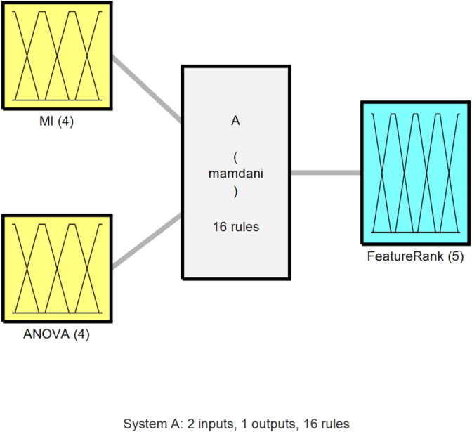
Proposed fuzzy model for ranking features based on the weights determined by MI and ANOVA.

According to Fig. 2, the proposed method utilizes a fuzzy inference system based on the Mamdani model. The ranking values determined by MI and ANOVA form the two inputs to this model. Various scenarios of the relationship between these two inputs for each feature are evaluated based on 16 rules to describe the importance of the corresponding input in the form of a fuzzy variable. Additionally, the membership functions for each of the input and output variables in the proposed fuzzy model for feature ranking are illustrated in Fig. 3.

According to the membership functions depicted in Fig. 3, the two input variables of the proposed fuzzy model have similar membership functions. Each input variable corresponds to the ranking values determined by each of the MI and ANOVA strategies, mapping the rank of each feature as a fuzzy number with four membership functions: low, approximately low, approximately high, and high. It is important to note that the rankings established by either of the two described strategies are mapped to the range [0,+1] using the min-max technique before being utilized in the proposed fuzzy model.

Trapezoidal membership functions were used for the fuzzy variables (inputs and output) of the proposed model. A trapezoidal membership function, denoted as , is defined by four parameters: a, b, c, and d. The membership degree of an element x to the fuzzy set A is given by Eq. (6)³⁴.

2

The Center of Gravity (CoG) method is used to defuzzify the fuzzy output and obtain a crisp weight value. This method is used for calculating the crisp value as the weighted average of the membership function values³⁴.

3

where is the crisp weight value and refers to the membership degree of the i-th rule’s output at weight w. In this method, the summation is over all fired rules. Based on the input fuzzy variables, the output of the fuzzy system, which indicates the importance of the feature, will be determined. The fuzzy ranking system functions through its rule base which is explained in detail in Table 2. The 16 rules stem from heuristic principles and expert reasoning about interpreting MI and ANOVA feature rankings.

The system maps two-dimensional input data consisting of normalized MI rank and ANOVA rank into a fuzzy output variable which represents feature importance. These rules establish a strong yet easily understandable combination between the two separate ranking systems. For instance, when both MI and ANOVA methods produce ‘High’ rankings the feature importance reaches a definitive conclusion at ‘Very High’. In contrast, the feature importance receives a rating of ‘Very Low’ when both methods provide ‘Low’ ranks. The intermediate rules of the proposed methodology handle all possible scenarios where ANOVA and MI produce different or unclear signals (e.g. ‘High’ and ‘Low’ ranks result in ‘Medium’ importance) to ensure both methods contribute their distinctive insights to the final feature importance evaluation. The rules mentioned in Table 2 determine the importance of each feature as a fuzzy variable with five membership functions: very low, low, medium, high, and very high.

At the end of the feature selection step, the BEFS strategy³⁵ is used to gradually eliminate irrelevant features. In this backward process, all candidate features are initially considered as a set of relevant indicators, and the classification model is trained based on these features to measure the training error with all candidate features. Then, a repeated process is employed to sequentially eliminate irrelevant features. During this process, the feature with the lowest Rank score is first removed from the selected feature set, and the learning model is trained based on the remaining indicators. The training error of the learning model is then measured based on the reduced set of features. If the new set results in a decrease in the training error of the model, the processes of feature elimination, training the model on that set, and evaluating the training error are repeated; otherwise, the feature elimination process concludes, and in this case, the subset of features that has resulted in the lowest training error is considered as the relevant features. This subset is used as input for the third phase of the proposed method.

The analysis of computational complexity determines the scalability of the proposed feature selection process. The first step of ranking requires computing MI and ANOVA F-scores for all features using samples. The computation of MI requires time while ANOVA F-score evaluation takes . The fuzzy inference system performs a subsequent combination of the obtained rankings. The computational efficiency of applying the defined fuzzy system to rank features using MI and ANOVA scores amounts to . BEFS performs an iterative process of evaluating feature subsets during its final stage. The system executes evaluation model training followed by performance assessment in every iteration. BEFS requires model training iterations because it potentially removes features one at a time. The computational complexity of BEFS equals the sum of for all values from 1 to (as ). The worst-case complexity of BEFS becomes when represents either average or maximum training time per iteration. BEFS becomes the primary factor determining overall complexity because it must perform model training iterations or because evaluation model training takes a long time. The fuzzy ranking process itself proves efficient but the iterative structure of BEFS becomes the main determinant of this feature selection stage’s scalability.

Deep neural network-based modelling

After the determination of the set of features relevant to students’ academic performance, an ensemble stack of deep learning models is used to predict the target variable. This ensemble stack consists of three models: CNN, LSTM, and MLP, each of which independently predicts the target variable based on the selected features. In the next step, the outputs of these three models are ensemble by a meta-model. This section elaborates on the structure of each of the three learning components in the proposed ensemble stack system.

a) Convolutional Neural Network.

The first to be used in the proposed ensemble stack for the prediction of students’ academic performance is the CNN. The CNN model used in the proposed method is a one-dimensional network that includes input layers, convolutional blocks for feature extraction, and the necessary layers for predicting the target variable. The overall structure of this CNN model is illustrated in Fig. 4.

Fig. 4.

Structure of the CNN model used in the proposed ensemble stack.

According to Fig. 4, the CNN model used in the proposed method consists of three convolutional blocks. In this CNN model, one-dimensional convolutional and pooling layers are employed to process the selected features. Consequently, it is natural that the input layer of this 1D CNN is defined as one-dimensional, accepting the extracted data from the previous step without alteration. Besides, the 1D CNN uses the sigmoid activation function for the first and second convolutional blocks, while the ReLU activation function is set for the third convolutional block. The CNN model concludes with the necessary layers to predict the target variable. In this context, two fully connected layers, with dimensions of 50 and 2 respectively, reduce the dimensions of the extracted feature maps, and ultimately, the student’s academic performance (score) is determined using a sigmoid layer with a single neuron.

To obtain the best efficiency in feature extraction, the CNN’s hyperparameters were tuned using a grid search technique. The hyperparameters related to the configuration of the CNN that were examined during the search include: filter size for each convolutional layer (with a search range of {2, 3, …, 12}), number of filters in the convolutional layer (with a search range of {8, 16, 24, 32, 48, 64}), type of activation function (which can be ReLU, Sigmoid, or Leaky ReLU), and type of pooling function (with options of Max, Min, Average). Furthermore, the model’s performance was evaluated across different training configurations, including the training algorithms Adam or SGDM and the minimum batch size. The search for configurations and the assessment of their fitness were conducted based on the validation error criterion. The training of the CNN model based on the SGDM optimizer with a minimum batch size of 32 yielded the best performance on the dataset used. For this optimal configuration, the specific hyperparameters included a learning rate of 0.005 and a momentum value of 0.95. The output of this CNN provides one of the input parameters for the meta-model in the ensemble stack system.

b) LSTM Network.

In the proposed ensemble stack, the LSTM stack is applied to model complex relationships between the selected features and students’ academic performance. As LSTM is capable of processing time sequences and keeping information for a long period of time, it is expected that this model will be able to predict students’ academic performance with more accuracy. In LSTM, the main processing units for features are memory cells, which have three gates:

• Input gate: Controls how much new information enters the memory cell.

• Forget gate: Controls how much of the stored information in the memory cell is discarded.

• Output gate: Controls how much of the stored information in the memory cell is passed to the output.

• In this model, the information from the input passes through each gate, which further gets processed through a sigmoid function. This gives an output value in between 0 and 1. It denotes the quantity of information to be passed through. The filtered information by the gates comes into the memory cell, and at last, the output of the memory cell is generated. The proposed modelling step uses a stack of LSTM layers instead of a single layer to analyse features at different levels of abstraction and then predict the target variable. This predictive component can be further broken down into the following components:

• First LSTM Layer: The first layer in the stack takes the pre-processed features as input. It processes each element of the sequence and learns the short-term dependencies in the represented window. This layer outputs the hidden state, which encapsulates relevant information extracted from the current steps and several time steps previously.

• Subsequent LSTM Layers: This hidden state is fed to the next LSTM layer in the stack. Further, this not only processes the current input sequence but also takes into consideration the information captured in the previous hidden state. This allows the network to learn not only immediate relationships within a window but also how these short-term dependencies evolve over longer periods.

• Output of the LSTM Stack: The last LSTM layer in the stack makes, after processing is complete with an entire sequence, an output through a dense layer; that forms the prediction for performance by a student entered through specifications.

The window length and the number of LSTM layers in the stack are the most critical hyperparameters to tune in the feature extraction model. Utilizing a deeper stack allows the model to capture more complex temporal patterns, but it also increases the complexity and risk of overfitting the model. Thus, in this study, the LSTM stack model was evaluated with various depths and window lengths, ultimately determining that using an LSTM stack with a depth of 5 and a window length of L = 15 could yield the best model performance.

c) MLP.

The third deep learning component in this proposed ensemble stack is a large MLP, the configuration of which involves two hidden layers that can predict student academic performance. This model consists of a total of four layers (input, two hidden layers, and one output layer). The input layer size is equal to the number of features selected in the second step of the proposed method.

The first hidden layer contains 13 neurons, which transfer their positive output values to the second hidden layer using the ReLU activation function, replacing negative values with zero. Additionally, the second hidden layer in this model consists of 9 neurons, and its activation function is set to sigmoid. Finally, the output layer of the MLP model, with a single neuron, specifies the predicted value for the target variable. The Levenberg-Marquardt Algorithm (LMA)³⁶ is used to train this model. The Levenberg-Marquardt Algorithm is a numerical optimization method used for solving nonlinear least squares problems. The overall performance of the LMA in training the MLP is as follows:

• Cost Function: LMA aims at the minimization of the cost function, which, in the proposed approach, is taken as the Mean Squared Error (MSE) criterion. This function calculates the mean squared difference between the predicted output and the actual output of the neural network.

• Weight Updates: During each step, LMA updates the weights and biases of the neural network using information derived from the gradient of the cost function.

• Learning Rate Determination: LMA uses a tunable parameter called the learning rate, which sets the size of the steps when weights are updated.

• Interpolation Between Newton and Gradient Descent Methods: LMA is an interpolation between the Newton approach (which is efficient for smooth problems near a local minimum) and the gradient descent method (which is more stable for irregular issues distant from a local minimum).

It is worth noting that during the model training process, the number of training cycles is set to 1000, and the threshold for the number of cycles leading to failure (no reduction in validation error) is set to 50.

Ensemble-based prediction

In the proposed method, the output of the ensemble system is determined by combining the weighted models of the deep models used in the third step. For this purpose, an MLP model is used as a super-model to provide a more accurate prediction of students’ academic performance by combining the outputs of the deep models. The proposed MLP model is a feedforward network with a single hidden layer that has seven neurons in its hidden layer and uses the tangent logistic function as the activation function in its layers.

The number of input neurons of the MLP model corresponds to the number of deep models present in the ensemble system, and the predicted output of each CNN, LSTM, and MLP model provides one of the input features for the super-model. The proposed model also includes one output neuron, which provides the overall forecasted value of the ensemble system for the student performance variable. In the proposed ensemble system, the super-model is trained by using the LMA algorithm based on the relationship between the outputs of deep models and the target variable. For this model, the number of training epochs is taken as 500, while the early stopping threshold is considered to be 30.

Research finding

The presented approach was implemented using MATLAB 2020a. To implement the comonents of the suggested model, we used the tools provided by “Deep Learning Toolbox” for implementing the prediction model; “Statistics and Machine Learning Toolbox” for preprocessing, MI/ANOVA calculations, and KNN imputation; and “Fuzzy Logic Toolbox” for implementation of the fuzzy logic system. The proposed method was implemented in different modes, each of which is described below. The Proposed mode is the same as the approach explained in Seciton 3. Instead, the Proposed mode (no FS) refers to a situation where the feature selection step using fuzzy logic is ignored, or in other words, all 30 input features are used to predict students’ academic performance. This comparison can show the impact and importance of the feature selection step on the performance of the model. Also, the Averaging mode refers to a situation where the averaging technique is used in the ensemble model.

In this scenario, the combination of the outputs of the three ensemble models, namely CNN, LSTM, and MLP, is used to create the final output. In this case, instead of taking the final prediction with the MLP meta-model, the average of the outputs is taken. This will clearly point out the effect of the usage of meta-model in the proposed method while comparing the proposed method in this mode. Finally, the CNN-LSTM mode refers to using a combination of CNN and LSTM for prediction only, which demonstrates the power of these two models in learning data features in combination. In addition, we used the methods of Beckham et al.²¹ and Liu et al.²² for comparison.

A rigorous evaluation of the proposed model utilized the dataset containing 628 student records according to “Data”. The evaluation process used a 10-fold cross-validation method to acquire a dependable performance evaluation that reduced sampling biases. Each cross-validation process fold divided its available data (90% of total data) into training (80%) and validation (10%) subsets. The 10% portion of data functioned as the independent test set for each fold. The model parameters were trained on the training set data but the validation set was exclusively used for adjusting CNN and LSTM components and implementing early stopping to avoid overfitting. The reported performance metrics emerge from averaging the results obtained from testing all 10 folds. A number of measures, including RMSE, MAPE, R Squared (R2), Concordance Correlation Coefficient (CCC), Spearman Rank Order Correlation Coefficient (SROCC), and Pearson Linear Correlation Coefficient (PLCC) have been used to assess the effectiveness of the suggested approach.

A measure of prediction accuracy, the RMSE is the square root of the average of squared discrepancies between actual and predicted values. It is expressed in the same unit as the data. Relative prediction accuracy is indicated by MAPE, which employs the average absolute percentage error, expressed as a percent, among the predictions and actual values.

4

5

Where represents the observed target variable, represents the predicted target variable, and N denotes the number of observations.

PLCC measures the linear relationship between two variables and then quantifies the strength and direction of their correlation. SROCC estimates the degree to which the relationship between two variables can be described using a monotonic function based on their ranks. The CCC expresses a measure of agreement between the two variable measurements, taking into account both their correlation and how much they conform to the line of equality. The R-squared in any regression model, R², is the proportion of variance in the dependent variable predictable by the independent variable or variables. In other words, it conveys a measure about the explanatory power of the model.

6

Where x and y are the two variables; and are the respective means; and N represents the number of observations.

7

Where is the difference in ranks for observation i, and n is the number of observations.

8

Where and are the standard deviations, and and are the means of the variables.

9

Where is the observed value, is the predicted value, and is the mean of the observed values.

Figure 5a demonstrates the ranking of features obtained through MI, ANOVA, and the fuzzy interference system through feature selection phase. It should be noted that this figure represents the results obtained through one of the experiment’s iterations.

Fig. 5.

Details of the selection of performance-related factors.

As shown in Fig. 5a, the MI and ANOVA show disagreements in ranking some of features. In this case, the FIS model attempts to provide an appropriate ranking by considering the ranking of both approaches. Figures 5b, and 5c illustrate the results of the presented feature selection strategy in various iterations of the experiment. In this figure, the feature selection process is examined in different iterations. In each of the 10 iterations of the experiment, features were selected individually; where yellow indicates feature selection and blue indicates feature deletion. Figure 5c displays the feature selection rate. The features selected in more than half of the experiment iterations are considered as relevant features. This feature selection method will enhance the model’s accuracy and reduce its complexity by including only those features that effectively predict student performance.

Figure 6 shows the error rate in the forecast using the RMSE chart. Figure 6a shows the RMSE of 10 iterations of the cross-validation for the proposed method and the compared methods. The proposed method retains the lowest RMSE values across the compared methods, hence the best in prediction. Whereas high RMSE, the Proposed method (no FS) indicates that feature selection has a vital contribution to increasing the model’s accuracy.

Fig. 6.

Performance evaluation of the proposed method (a) RMSE values in each iteration and (b) boxplot of RMSE.

The Averaging and CNN-LSTM methods show moderate performance, while the results of the comparison methods Beckham et al.²¹ and Liu et al.²² show higher RMSE values, indicating that the proposed method provides significantly more accurate predictions. The results indicate that this figure emphasizes the effectiveness of the proposed method in reducing prediction errors, especially when feature selection is performed. Figure 6b is a boxplot that displays the distribution of RMSE values for different methods of predicting academic achievement and clearly shows statistical features such as median and quartiles. In this figure, the proposed method has the lowest RMSE value, indicating its superior performance. Also, the boxplot between the first and third quartiles can confirm the consistency of the results of this method since the proposed method has a lower error value than the other compared methods.

The Averaging method also has the highest RMSE and the widest box, indicating its inefficiency in providing accurate predictions. The RMSE values calculated for the CNN-LSTM models and the results of the comparative methods Beckham et al.²¹ and Liu et al.²² that are outside the desired range indicate their lower performance than the proposed method. The results show that the proposed method not only has less error but also provides greater accuracy and stability in predictions, which makes it an effective tool for predicting students’ academic success.

Figure 7 shows the error rate in the forecast using the MAPE chart. Figure 7a depicts the results of the proposed method and the compared methods in 10-folds using the MAPE criterion. It is clear that the performance of the proposed method is better than that of any other method. Besides, its MAPE value is steadily at the lowest level. This indicates the high accuracy of the proposed method in predicting academic achievement. The Average methods and the Beckham et al.²¹ and Liu et al.²² models also show different results; however, none of the compared methods can come close to the accuracy of the proposed method.

Fig. 7.

Performance evaluation of the proposed method (a) MAPE values in each iteration and (b) boxplot of MAPE.

The result shows that the proposed approach not only is better but also enhances its predictive ability with increasing iterations. Figure 7b discusses the MAPE values of the different models by a boxplot. The figure shows that, among the different models, the proposed one has a noticeably lower MAPE, which corresponds to significant differences in the precision of the predictions. The Average method exhibits the highest average error, which indicates the inability of this method to predict more accurately. Also, the Beckham et al.²¹ and Liu et al.²² models are in a similar position, and their MAPE is close to each other and higher than the proposed method. The variance and the size of the box clearly indicate that, not only is the proposed method more accurate but it also has less variation, which indeed points to the stability and reliability of the model under different conditions. These results confirm that the proposed model has superior accuracy in the prediction of students’ academic success.

Figure 8 shows the regression plot. It is explicitly observed from the regression diagram of actual outputs against the predicted output by the different models that the high performance of the proposed method is apparent. The fit line related to the proposed model is the one that is closer to aligning with the equivalent y-line, i.e., actual outputs, which proximity reflects accuracy in the predictions. Also, the correlation between the predicted outputs and the target values, referred to as R, is much closer to one for the proposed method when compared to other methods. This increased correlation and closer alignment signify a reduction in error and an increase in the accuracy of the predictions, resulting from effective feature selection and the ensemble of different neural networks under a meta-model in the ensemble system. This will prove that the proposed approach works effectively in improving performance in predicting students’ academic success.

Fig. 8.

Regression plots of the proposed method compared to other scenarios.

Figure 9 shows the prediction of students’ academic success based on the PLCC, SROCC, CCC, and R-squared measures. The PLCC reflects the strength and direction of the linear relationship between predicted and actual values, reflecting strong predictive capability when higher. SROCC assesses the monotonic relationship, underlining the robustness of the model against nonlinearities and outliers. The CCC computes how well the predicted values conform to the actual values, with emphasis on precision. R² gives the fraction of variance in the observed outcomes explained by the model. Thus, the higher values correspond to the best fit. Put altogether, these metrics show the proposed method’s efficiency in the best prediction of students’ performance and catching relevant trends in the data.

Fig. 9.

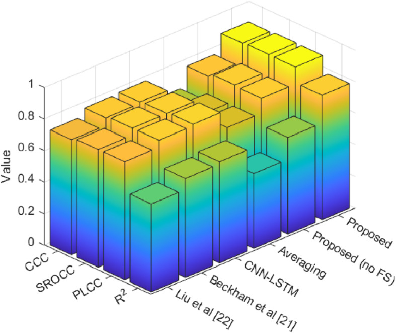
Evaluation of the performance of the proposed method using PLCC, SROCC, CCC and R-squared metrics.

Figure 10 shows a Taylor diagram comparing different methods based on three critical criteria, namely standard deviation, RMSE, and the correlation coefficient. The proposed method has attained a critical achievement because it has lower RMSE and standard deviation values, which means the prediction it will make will be more accurate and stable compared to the other methods.

Fig. 10.

Taylor diagram of the proposed method and different scenarios for predicting the target variable.

Furthermore, the higher correlation coefficient underlines that the outputs produced by the suggested method are closer to real target values. This combination of reduced error metrics and improved correlation highlights the effectiveness of the proposed approach by demonstrating its superiority in accurately predicting students’ academic success, with an emphasis on the benefits of the ensemble feature selection and neural network ensemble strategy.

Table 3 compares the performance of the proposed method against other methods, without feature selection of the proposed method, averaging, a combination of CNN and LSTM, and previous results using Beckham et al.²¹ and Liu et al.²² Indeed, the obtained results indicate that the proposed method has outperformed other methods with minimum RMSE and MAPE values of 1.4908 and 0.0895, respectively, and the proposed method was significantly better compared to others. Not applying feature selection in the Proposed (no FS) method increases errors and reduces accuracy. Also, the averaging method shows the weakest result: RMSE − 3.0572, MAPE − 0.1864. In general, this table confirms that the proposed method outperforms other methods in terms of the accuracy of prediction and identification of effective features.

Table 3.

Summary of the comparison results of the proposed method and the compared methods.

Methods	RMSE	MAPE	R squared	PLCC	SROCC	CCC
Proposed	1.4908	0.0895	0.7890	0.8883	0.8900	0.8835
Proposed (no FS)	2.2245	01348	0.6120	0.7823	0.7890	0.7676
Averaging	3.0572	0.1864	0.4737	0.6883	0.6897	0.6444
CNN-LSTM	2.1335	0.1280	0.6411	0.8007	0.7914	0.7849
Beckham et al. 21	2.1777	0.1318	0.6260	0.7912	0.7895	0.7763
Liu et al.22	2.4206	0.1455	0.5568	0.7462	0.7452	0.7295

The Fig. 11 demonstrates the generalization ability along with overfitting risk assessment through training and validation RMSE curves of our individual deep learning models (MLP, CNN, BiLSTM). The performance of all models over both training and validation data appears through these curves during the 100 epochs of training.

Fig. 11.

Training and validation loss curves for the (a) MLP, (b) CNN, and (c) BiLSTM models.

All three models (MLP, CNN, and BiLSTM) demonstrate a decreasing training RMSE (red line) during training which proves their ability to minimize errors on training data. The validation RMSE (blue line) reduces its value while following the training RMSE (red line) throughout model training.

The validation RMSE shows minimal variations in its curve during the later epochs without experiencing substantial growth as the training RMSE continues its downward trajectory. The pattern demonstrates both general model performance on new data and avoidance of severe overfitting during the training period. The similar shapes of validation and training RMSE curves support the conclusion that the models found meaningful patterns in the features instead of memorizing training examples. The adequate performance of base models proves their resistance to overfitting thereby making the overall proposed stacked ensemble method more accurate.

The proposed stacked ensemble method underwent statistical analysis that allowed researchers to assess its performance improvements through RMSE and MAPE results by comparing them with baseline methods. The non-parametric Friedman test served to perform this analysis³⁷. The test establishes whether statistical differences exist between the median results of the examined methods.

The evaluation took place independently for RMSE and MAPE measurement methods. The test set samples function as individual ‘blocks’ for evaluating different model performances. The models received rankings based on their performance results for each sample through the evaluation of RMSE and MAPE metrics. The model achieving the lowest error received rank 1 followed by rank 2 for the second-best model and so on.

The Friedman test examines which states that prediction methods demonstrate equivalent performance through comparable median error measures (RMSE or MAPE). The statistical test rejects () to show that the models demonstrate different performance levels.

Table 4 shows the results obtained from conducting the Friedman test. Using RMSE as the metric the Chi-squared statistic from the test reached 31.52 with 4 degrees of freedom producing a p-value of . The Friedman test analysis for MAPE metric produced a Chi-squared statistic value of 33.68 with a p-value of . The null hypothesis receives rejection from the analysis of both RMSE and MAPE results. The performance distributions between the examined prediction models show statistically meaningful variations according to the results.

Table 4.

The results of analysis on the RMSE and MAPE metric.

	RMSE					MAPE
	SS		MS			SS		MS
Columns	78.8	4	19.7	31.52		84.2	4	21.05	33.68
Error	21.2	36	0.5889			15.8	36	0.4389
Total	100	49				100	49

A post-hoc analysis becomes necessary because the Friedman test established significant overall differences between the models. We conducted pairwise comparisons through the Nemenyi post-hoc test³⁷. The Nemenyi test evaluates method performance by comparing their average ranks while two methods show significant differences when their average rank values exceed the Critical Difference (CD) which equals , where k shows the number of compared cases, N is the sample size, and is the critical value based on the Studentized range statistic divided by .

The post-hoc results appear in Fig. 12 through a CD diagram representation. The graphical representation displays models through their average ranking positions with better performance at lower positions. The horizontal bar represents the calculated CD and models with average ranks beyond this value demonstrate statistical significance for differences.

Fig. 12.

Multiple comparison analysis on the (a) RMSE, and (b) MAPE.

The CD diagrams of Fig. 12-a display RMSE performance while Fig. 12-b shows MAPE performance of the methods. The proposed method obtained the best average ranking position across both evaluation metrics. The proposed method achieves a statistically significant lower (better) average rank than “no FS” and “Averaging” and “Liu et al.²²” for both RMSE and MAPE based on post-hoc analysis because their rank differences surpass the CD threshold. The proposed method demonstrated superior performance compared to “Beckham et al.²¹” but this difference proved non-significant during the α = 0.05 statistical test.

Conclusion

This paper presented a new method of predicting academic performance, combining a four-step process: data preprocessing, feature selection using fuzzy logic, modeling by deep neural networks, and extracting the target variable through a meta-model. The obtained results with this approach highly improved the performance prediction accuracy, reducing the prediction errors in metrics of RMSE and MAPE to 0.6 and 0.03%, respectively. This approach allows not only for the identification of the needs and weaknesses of each student but also for the elaboration of an educational program based on the performance of the students. This tool will help teachers and educational administrators to identify, with anticipation, possible academic problems for the continuous improvement of the students’ performance. The proposed model enables several practical real-world applications which include:

1. The first solution entails creating predictive student alert systems which determine students prone to low achievement allowing for immediate professional guidance.

2. Academic advisors receive valuable data-based student information for more customized and efficient guidance of their students.

3. This model supports institutional resource allocation decisions for academic support programs through its data outputs.

4. The model provides essential information which helps review curricula and make adjustments based on predictors that strongly affect student success.

Therefore, the given method can serve as an efficient tool for improvement in educational quality and optimization of learning processes in an educational environment.

Limitations and future works

Here, the limitations of the research as well as future directions in this field are examined:

• Data Scope and Generalizability: The main data constraint stems from using questionnaires to gather information from Nanjing China-based engineering students at universities. The model demonstrates effectiveness within Chinese engineering students in Nanjing universities but its validity for larger educational populations in diverse cultural groups across multiple educational systems and geographical areas needs further confirmation. Contextual differences produce substantial variations in the elements that affect academic performance. Future studies must analyze the proposed model’s performance through inspections of datasets that include students from multiple institutions across different regions. The model must be adapted through local data retraining to achieve effective performance across different educational settings.

• Computational Complexity: The second limitation involves computational complexity. This method has employed a number of deep learning models, and these consume more processing load while working independently. The sum of these models leads to a massive increase in processing load compared to other methods. Although this increase in processing load is visible in the training phase, in future research, this problem can be reduced in the training phase by using methods that increase computational efficiency such as hardware accelerators, the use of parallel processing and other techniques to improve the performance of deep models, such as quantization.

• Model Interpretability: The prediction accuracy of the stacked ensemble model makes interpretation difficult because the system consists of multiple deep learning components which result in complexity. For educational use and user trust it is vital to understand what factors result in specific predictions made by the model. Researchers should investigate the implementation of model-agnostic interpretation tools among LIME (Local Interpretable Model-agnostic Explanations) and SHAP (SHapley Additive exPlanations) to enhance explainability of the prediction system. The methods would deliver important findings by measuring how each selected input feature from fuzzy feature selection affects individual student academic performance predictions thus revealing essential model outcome determinants.

Author contributions

Jiawei Gu the main manuscript text. Jiawei Gu reviewed the manuscript.

Funding

This work was suported by The second Hang Yanpei vocational Education Thought Research Pianning Prject of china ocational Education sociely (CVES) Research on eacher CompetencDevelopment under the Guidance of Huang Yanpei’s View of Vocational Education Teachers’ (ZJS2024ZN038) and 2024 Hainan Provincial Education Science Planning General Project Title: Construction of Moral Education Knowledge System and Innovation of Educational Practice Empowered by Artificial Intelligence: Tradition and Modernity Exploring Paths of Educational Integration Project Number: QJY202412207.

Data availability

The dataset generated and analyzed during the current study will be made available in a public repository upon publication of this article.

Declarations

Competing interests

The authors declare no competing interests.

References

- 1.Singh, R. & Pal, S. Machine learning algorithms and ensemble technique to improve prediction of students performance. Int. J. Adv. Trends Comput. Sci. Eng.9(3). (2020).
- 2.Talal, H. & Saeed, S. A study on adoption of data mining techniques to analyze academic performance. ICIC Express Lett. Part. B: Appl.10 (8), 681–687 (2019). [Google Scholar]
- 3.Yaacob, W. F. W., Nasir, S. A. M., Yaacob, W. F. W. & Sobri, N. M. Supervised data mining approach for predicting student performance. Indones J. Electr. Eng. Comput. Sci.16 (3), 1584–1592 (2019). [Google Scholar]
- 4.Almasri, A., Celebi, E. & Alkhawaldeh, R. S. EMT: ensemble meta-based tree model for predicting student performance. Sci. Program.2019 (1), 3610248 (2019). [Google Scholar]
- 5.El Aissaoui, O., Madani, E. A. E., Oughdir, Y., Dakkak, L. & Allioui, E. A., Y. A multiple linear regression-based approach to predict student performance. In International Conference on Advanced Intelligent Systems for Sustainable Development. 9–23. (Springer, 2019).
- 6.Khashman, A. & Carstea, C. G. Oil price prediction using a supervised neural network. Int. J. Oil Gas Coal Technol.20 (3), 360–371 (2019). [Google Scholar]
- 7.Sekeroglu, B. & Tuncal, K. Prediction of cancer incidence rates for the European continent using machine learning models. Health Inf. J.27 (1), 1460458220983878 (2021). [DOI] [PubMed] [Google Scholar]
- 8.Özçil, İ. E., Esenyel, I. & Ilhan, A. A fuzzy approach analysis of Halloumi cheese in N. Cyprus. Food. Anal. Methods. 15 (1), 10–15 (2022). [Google Scholar]
- 9.Sekeroglu, B., Abiyev, R., Ilhan, A., Arslan, M. & Idoko, J. B. Systematic literature review on machine learning and student performance prediction: critical gaps and possible remedies. Appl. Sci.11 (22), 10907 (2021). [Google Scholar]
- 10.Batool, S. et al. Educational data mining to predict students’ academic performance: A survey study. Educ. Inform. Technol.28 (1), 905–971 (2023). [Google Scholar]
- 11.Hussain, S. & Khan, M. Q. Student-performulator: predicting students’ academic performance at secondary and intermediate level using machine learning. Annals Data Sci.10 (3), 637–655 (2023). [DOI] [PMC free article] [PubMed] [Google Scholar]
- 12.Mallak, S. et al. Using Markov chains and data mining techniques to predict students’ academic performance. Inf. Sci. Lett.12 (9), 2073–2083 (2023). [Google Scholar]
- 13.Issah, I., Appiah, O., Appiahene, P. & Inusah, F. A systematic review of the literature on machine learning application of determining the attributes influencing academic performance. Decis. Analytics J.7, 100204 (2023). [Google Scholar]
- 14.Pallathadka, H. et al. Classification and prediction of student performance data using various machine learning algorithms. Mater. Today: Proc.80, 3782–3785 (2023). [Google Scholar]
- 15.Nurudeen, M., Abdul-Samad, S., Owusu-Oware, E., Koi-Akrofi, G. Y. & Tanye, H. A. Measuring the effect of social media on student academic performance using a social media influence factor model. Educ. Inform. Technol.28 (1), 1165–1188 (2023). [Google Scholar]
- 16.Arizmendi, C. J. et al. Predicting student outcomes using digital logs of learning behaviors: Review, current standards, and suggestions for future work. Behav. Res. Methods. 55 (6), 3026–3054 (2023). [DOI] [PMC free article] [PubMed] [Google Scholar]
- 17.He, P. et al. Predicting student science achievement using post-unit assessment performances in a coherent high school chemistry project‐based learning system. J. Res. Sci. Teach.60 (4), 724–760 (2023). [Google Scholar]
- 18.Acosta-Gonzaga, E. The effects of self-esteem and academic engagement on university students’ performance. Behav. Sci.13 (4), 348 (2023). [DOI] [PMC free article] [PubMed] [Google Scholar]
- 19.Abid, N., Aslam, S., Alghamdi, A. A. & Kumar, T. Relationships among students’ reading habits, study skills, and academic achievement in English at the secondary level. Front. Psychol.14, 1020269 (2023). [DOI] [PMC free article] [PubMed] [Google Scholar]
- 20.Murnawan, M., Lestari, S., Samihardjo, R. & Dewi, D. A. Sustainable educational data mining studies: identifying key factors and techniques for predicting student academic performance. J. Appl. Data Sci.5 (3), 1325–1342 (2024). [Google Scholar]
- 21.Beckham, N. R., Akeh, L. J., Mitaart, G. N. P. & Moniaga, J. V. Determining factors that affect student performance using various machine learning methods. Procedia Comput. Sci.216, 597–603 (2023). [Google Scholar]
- 22.Liu, C., Wang, H. & Yuan, Z. A method for predicting the academic performances of college students based on education system data. Mathematics10 (20), 3737 (2022). [Google Scholar]
- 23.Mohd Zaki, S. et al. N. Predicting students’ performance at higher education institutions using a machine learning approach. Kybernetes (2024).
- 24.Chukwu, G. C. et al. Design and Implementation of an Expert System for Predicting Students’ Academic Performance (A Case Study of Computer Science Department Federal Polytechnic Bida, 2024).
- 25.Yau, S., Ishola, A. A. & Adamu, A. I. Predicting the effect of mobile phone on student academic performance using machine learning. Int. J. Sci. Res. Comput. Sci. Eng.12(5). (2024).
- 26.Aziz, R., Verma, C. & Srivastava, N. A fuzzy based feature selection from independent component subspace for machine learning classification of microarray data. Genomics Data. 8, 4–15 (2016). [DOI] [PMC free article] [PubMed] [Google Scholar]
- 27.Joshi, A. A. & Aziz, R. M. Soft computing techniques for cancer classification of gene expression microarray data: A three-phase hybrid approach. In Computational Intelligence for Data Analysis. 92–113. (Bentham Science, 2024).
- 28.Afreen, S., Bhurjee, A. K. & Aziz, R. M. Feature selection using game Shapley improved grey Wolf optimizer for optimizing cancer classification. Knowl. Inf. Syst. 1–32 (2025).
- 29.Afreen, S., Bhurjee, A. K. & Aziz, R. M. Cancer classification using RNA sequencing gene expression data based on game Shapley local search embedded binary social ski-driver optimization algorithms. Microchem. J.205, 111280 (2024). [Google Scholar]
- 30.Sharma, A., Kumar, P., Ben, D., Bikhani, M. & Aziz, R. M. Improved GA based clustering with a new selection method for categorical dental data. In Swarm Optimization for Biomedical Applications. 172–192. (CRC, 2025).
- 31.Crowther, P. & Briant, S. Predicting academic success: A longitudinal study of university design students. Int. J. Art Des. Educ.40 (1), 20–34 (2021). [Google Scholar]
- 32.Vergara, J. R. & Estévez, P. A. A review of feature selection methods based on mutual information. Neural Comput. Appl.24, 175–186 (2014). [Google Scholar]
- 33.Henson, R. N. Analysis of Variance (ANOVA). Brain Mapping: An Encyclopedic Reference. 477–481 (Elsevier, 2015).
- 34.Zadeh, L. A. Fuzzy logic. In Granular, Fuzzy, and Soft Computing. 19–49. (Springer US, 2023). [Google Scholar]
- 35.Farahdiba, S., Kartini, D., Nugroho, R. A., Herteno, R. & Saragih, T. H. Backward elimination for feature selection on breast cancer classification using logistic regression and support vector machine algorithms. IJCCS (Indonesian J. Comput. Cybernetics Systems). 17 (4), 429–440 (2023). [Google Scholar]
- 36.Sapna, S., Tamilarasi, A. & Kumar, M. P. Backpropagation learning algorithm based on Levenberg Marquardt algorithm. Comp. Sci. Inf. Technol. (CS IT). 2, 393–398 (2012). [Google Scholar]
- 37.Demšar, J. Statistical comparisons of classifiers over multiple data sets. J. Mach. Learn. Res.7 (Jan), 1–30 (2006). [Google Scholar]
Associated Data
This section collects any data citations, data availability statements, or supplementary materials included in this article.
Data Availability Statement