A Constrained-Likelihood Approach to Marker-Trait Association Studies

Abstract

Marker-trait association analysis is an important statistical tool for detecting DNA variants responsible for genetic traits. In such analyses, an analysis model of the mean genetic effects of the genotypes is often specified. For instance, the effect of the disease allele on the trait is often specified to be dominant, recessive, additive, or multiplicative. Although this model-based approach is powerful when the analysis model is correctly specified, it has been found to have low power sometimes when the specified model is incorrect. We introduce an approach that does not require the specification of a particular genetic model. This approach is built upon a constrained maximum likelihood in which the mean genetic effect of the heterozygous genotype is required to not exceed those of the two homozygous genotypes. The asymptotic distribution of the likelihood-ratio statistic is derived for two special cases. A simulation study suggests that this new approach has power comparable to that of the model-based method when the analysis model is correctly specified. This approach uses one marker at a time (i.e., it is a single-marker analysis). However, given the latest findings that powerful inferential procedures for haplotype analyses can be constructed from single-marker analyses, we expect this approach to be useful for haplotype analyses.

Introduction

Marker-trait association analysis is an important statistical tool for detecting DNA variants responsible for genetic traits. It can provide higher mapping resolution than do methods based on closely related meiosis events. In such analyses, it is common to specify an analysis model of the average genetic effects of the genotypes. For instance, the effect of the disease allele on the trait is often specified to be dominant, recessive, additive, or multiplicative. When the specified model is close to the underlying trait model, this model-based approach provides a powerful means of detecting association. However, when the specified model is different from the underlying model, its power may be low (Slager and Schaid 2001; Freidlin et al. 2002; Schaid et al. 2005). In real-data analyses, the underlying genetic model is often unknown. For instance, one promising approach to investigation of the gene-regulation mechanism is to map the expression levels of genes by treating them as quantitative traits (Brem et al. 2002; Schadt et al. 2003; Yvert et al. 2003; Morley et al. 2004). Currently, gene-expression arrays contain thousands of DNA probes, and each probe provides a quantitative measurement of its expression level. Given this large number of traits, the model-based method may miss many true-positive signals. It is desirable to develop methods that have power for a wide range of genetic models.

Analytical methods that have power for a wide range of genetic models are desired not only for single-marker analysis but also for haplotype analysis in which multiple markers are involved. Some recent developments indicate that single-marker tests can be used to construct powerful inference procedures for haplotype analysis. Chapman et al. (2003) found that regression analysis based on a linear combination of tagSNPs is more powerful than the traditional haplotype analysis that is based on haplotype frequencies. Roeder et al. (2005) further found that inferential procedures based on single-marker tests, after correction for multiple testing by permutation or curve fitting, is at least as powerful as the regression method proposed by Chapman et al. (2003). In a more recent study, Schaid et al. (2005) described a testing procedure for haplotype analysis that requires specification of a “kernel.” One promising way of specifying a kernel is to derive it from single-marker tests (Schaid et al. 2005).

There have been some studies, mostly on dichotomous traits, that have investigated methods that do not rely on a particular analysis model. Freidlin et al. (2002) proposed a maximin efficiency robust test and a test (named “MAX”) based on the maximum of test statistics under several analysis models. They found that the MAX test is generally more powerful than the other one. Freidlin et al. (2002) assumed an a priori ordering of the mean genetic effects for the three genotypes that are induced from the allele to be tested, by assuming that the marker allele associated with the disease allele is known. Such an ordering can be difficult to make—for instance, in the expression-level mapping example mentioned above. To remove this restriction, Zheng (2003) proposed a “max and min scores” approach. Another method that does not require the specification of an analysis model is to simply compare mean genotypic effects by use of standard statistical methods such as analysis of variance. But such an approach may have low power due to increased degrees of freedom.

Instead of deriving tests from several model-based statistics or simply comparing the mean genotypic effects, we adopt a constrained-likelihood analysis under a so-called no-overdominance constraint. This constraint requires that the mean genetic effect of the heterozygous genotype not exceed those of the two homozygous genotypes—that is, it is neither larger than the larger of the mean genetic effects of the two homozygous genotypes nor smaller than the smaller of the two. We note that this constraint is satisfied by the commonly assumed analysis models—dominance, recessive, additive, and multiplicative.

In the following section, we introduce our approach in terms of a generalized linear model. We then apply this approach to quantitative traits and dichotomous traits. The asymptotic distribution of the constrained likelihood-ratio statistic for each kind of trait is introduced. Simulation studies were conducted to assess the performance of our method, under different generating models, in comparison with some popular methods. Technical details are given in appendixes A and B.

Methods

Let A denote the allele being tested for association with a trait. The three genotypes induced from allele A are indexed by j (j=0,1,2), where j is the number of copies of allele A. Denote the population frequency of genotype j by p_j. In some situations, the values of p_j are known. For instance, for the F₂ population, p₀=p₂=0.25 and p₁=0.5. Suppose that there are n_j individuals with genotype j. Given the total number of individuals n:=n₀+n₁+n₂, the triplet (n₀,n₁,n₂) follows a trinomial distribution with a parameter vector (p₀,p₁,p₂). The trait value of the ith individual of genotype j is denoted by y_ji. For dichotomous traits, it is defined that y_ji=1 for cases and y_ji=0 for controls. The sample mean for genotype j is denoted by .

Consider the following generalized linear model for phenotype y with link function g(·): E(y)=μ and g(μ)=α+δ₁x₁+(δ₁+δ₂)x₂, where x_j, j=1,2, is an indicator of genotype j satisfying x_j=1 if the individual is of genotype j and x_j=0 otherwise. Depending on the random component of the generalized linear model, there may be another nuisance parameter β (possibly a vector). For instance, for normal data, β is the variance of the random component. In the constrained-likelihood approach introduced here, we require a “no-overdominance” constraint on the three mean genotypic effects. That is, the three genotypic means satisfy either α⩽α+δ₁⩽α+δ₁+δ₂ or α⩾α+δ₁⩾α+δ₁+δ₂. This constraint implies that δ₁ and δ₂ cannot be of different signs, and it can be equivalently written δ₁δ₂⩾0, which corresponds to the first and third quadrants on the δ₁-δ₂ plane. When there is no association for allele A, δ₁=δ₂=0. Let Θ₀={(δ₁,δ₂,α,β):δ₁=δ₂=0} and Θ₁={(δ₁,δ₂,α,β):δ₁δ₂⩾0}. The hypotheses of interest are

The other parameters p₀, p₁, p₂, α, and β are nuisance parameters. The requirement δ₁δ₂⩾0 contains many commonly used genetic models as special cases. For instance, when the effect of allele A is dominant, we have δ₂=0, and there is no restriction on δ₁. When the effect of allele A is recessive, we have δ₁=0, and there is no restriction on δ₂.

The likelihood function of the data {y_ji} is

where L₁(p₀,p₁,p₂)=Pr(n₁,n₂,n₃|p₀,p₁,p₂,n) is the trinomial probability of (n₁,n₂,n₃), given n, and where L₂(δ₁,δ₂,α,β)=j=02i=1n_jPr(y_ji|δ₁,δ₂,α,β) is the conditional probability of the trait values {y_ji}, given (n₁,n₂,n₃).

The hypotheses in (1) can be tested using the likelihood-ratio statistic. Since L₁(p₀,p₁,p₂) and L₂(δ₁,δ₂,α,β) involve two nonoverlapping sets of parameters and since only L₂(δ₁,δ₂,α,β) contains the parameters of interest, the likelihood-ratio statistic equals

where l₂(δ₁,δ₂,α,β)=log[L₂(δ₁,δ₂,α,β)] and . The nuisance parameters p₀, p₁, and p₂ do not appear in the calculation of Λ_New. However, we show below that the asymptotic distribution of Λ_New can depend on p₀, p₁, and p₂.

To compute Λ_New, it is essential to compute the constrained maximum of l₂(δ₁,δ₂,α,β). For this purpose, define

to be the likelihood-ratio statistic for the dominance model and

to be the likelihood-ratio statistic for the recessive model. Further define Λ_Larger=max{Λ_Dom,Λ_Rec}. In principle, the constrained maximum of l₂(δ₁,δ₂,α,β) is straightforward to compute. According to standard optimization theory, there are two possible situations regarding the optimal values of δ₁ and δ₂. They are either in the interior of the region satisfying δ₁δ₂>0 or on the border of this region. The constrained maximum of l₂(δ₁,δ₂,α,β) equals its unconstrained maximum in the former case and equals Λ_Larger in the latter case.

Specifically, the constrained maximum of l₂(δ₁,δ₂,α,β) can be obtained as follows. Do the unconstrained maximization of l₂(δ₁,δ₂,α,β), and denote the values of δ₁, δ₂, α, and β for which l₂(δ₁,δ₂,α,β) is maximized by , and , respectively. The constrained maximum of l₂(δ₁,δ₂,α,β) equals if and equals Λ_Larger otherwise.

Next, we discuss two particular applications of this constrained-likelihood approach, one to quantitative traits and the other to dichotomous traits. For each application, the asymptotic distribution of the likelihood-ratio statistic Λ_New is derived. There should be many other possible applications, depending on the specification of the random component and the link function of the generalized linear model.

Quantitative Traits

Quantitative traits are usually modeled through a normal distribution, and the “canonical” link function is the identity function g(μ)=μ. Assume that the variance of the normal distribution is the same, regardless of the genotype, and denote this common variance by σ². The parameter σ² corresponds to the nuisance parameter β in our generalized-linear-model setup. Now, the function l₂ becomes

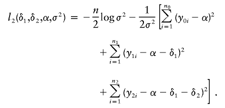The unconstrained maximum-likelihood estimates of α, δ₁, δ₂, and σ² are , , , and

respectively. For the recessive model (δ₁=0), the maximum-likelihood estimates of α and δ₂ are and , respectively. For the dominance model (δ₂=0), the maximum-likelihood estimates of α and δ₁ are and , respectively. The variance σ² is estimated by fixing (for the recessive model) or (for the dominance model) in equation (2). Under the null hypothesis, we have δ₁=δ₂=0, and the maximum-likelihood estimate of α is . Given these results, it is straightforward to compute the statistic Λ_New.

Let γ=(p₀p₂)^1/2[(1-p₀)(1-p₂)]^-1/2 and κ=(2π)^-1arccos(γ). In appendix A, it is shown that, as n→∞,

where (z₁,z₂)^t follows a standard bivariate normal distribution with correlation coefficient γ and where χ²₂ follows a χ² distribution with 2 df. It is also shown in appendix A that, as n→∞,

The statistic Λ_Larger was proposed as a robust test statistic (Freidlin et al. 2002), but its asymptotic distribution was not given. The correlation coefficient γ depends on the genotype frequencies p₀ and p₂. When their true values are unknown, the genotype frequencies p₀ and p₂ can be consistently estimated by their respective sample frequencies.

Dichotomous Traits

Dichotomous traits are usually modeled through binomial distribution, and the “canonical” link function is the logit function g(μ)=log[μ/(1-μ)]. In this situation, the log-likelihood function l₂ becomes, up to an additive constant,

where f₀:=exp(α)/[1+exp(α)], f₁:=exp(α+δ₁)/[1+exp(α+δ₁)], and f₂:=exp(α+δ₁+δ₂)/[1+exp(α+δ₁+δ₂)] are the penetrances of the trait for the three genotypes that have 0, 1, and 2 copies of allele A, respectively. We note that the Armitage trend test typically assumes δ₁=δ₂ (Sasieni 1997).

The likelihood function l₂(δ₁,δ₂,α) depends on δ₁, δ₂, and α through f₀, f₁, and f₂. The constraint δ₁δ₂⩾0 holds if and only if f₀⩾f₁⩾f₂ or f₀⩽f₁⩽f₂ holds. It is easy to obtain that the unconstrained maximum-likelihood estimate of f_j is , j=0,1,2. For the dominance model where f₁=f₂ (equivalent to δ₂=0), the maximum-likelihood estimate of f₀ is , and the maximum-likelihood estimate of f₁=f₂ is . For the recessive model where f₀=f₁ (equivalent to δ₁=0), the maximum-likelihood estimate of f₀=f₁ is , and the maximum-likelihood estimate of f₂ is . Under the null hypothesis, we have f₀=f₁=f₂, and the maximum-likelihood estimate is . Given these results, it is again straightforward to compute the statistic Λ_New.

The generalized linear model is appropriate for population samples. For selected samples such as cases and controls, it may not be appropriate. However, it has been shown that simply applying logit regression to case-control data affects only the intercept term α and not the slopes δ₁ and δ₂ (Prentice and Pyke 1979). Following the arguments of Prentice and Pyke (1979), it can be shown that the intercept term depends on δ₁, δ₂, and α and that the constraint δ₁δ₂⩾0 has no impact on the value the intercept term can take (details omitted). So, for a case-control study, one can treat the data as if they were population samples and apply the proposed test.

In appendix B, it is shown that the asymptotic distribution of Λ_New in this situation is identical to that of the likelihood-ratio statistic Λ_New for continuous traits. When true values are unknown, the genotype frequencies p₀ and p₂ can be estimated by their respective sample frequencies in the combined sample of cases and controls.

Let p denote the frequency of allele A. Under the assumption of Hardy-Weinberg equilibrium (HWE), some quantiles of the asymptotic distribution for Λ_New are tabulated in table 1 for p=0.01, 0.1, 0.3, and 0.5. We note that, for p=0.5, the genotype frequencies are p₀=p₂=0.25 and p₁=0.5, which are the expected genotype frequencies for the F₂ population.

Table 1.

Some Quantiles for Test Statistics Λ_New and Λ_Larger^[Note]

	Statistic atNominal Significance Level
Frequencyof Allele Aand Statistic	.1	.05	.01	.001
p=.01:
ΛNew	4.197	5.507	8.597	13.084
ΛLarger	3.796	5.000	7.874	12.115
p=.1:
ΛNew	4.152	5.457	8.536	13.008
ΛLarger	3.778	4.985	7.867	12.113
p=.3:
ΛNew	4.111	5.413	8.485	12.949
ΛLarger	3.752	4.964	7.855	12.109
p=.5:
ΛNew	4.100	5.401	8.472	12.934
ΛLarger	3.745	4.957	7.852	12.107

Note.— HWE is assumed, so that p₀=(1-p)², p₁=2p(1-p), and p₂=p².

Simulation

Simulation studies were done for both quantitative traits and dichotomous traits. The type I error rate and the power were computed on the basis of 10,000 replications.

Quantitative Traits

Consider the following data-generating model:

where G is the genotypic value and ε is an independent environmental factor. Let G=-a for genotype 0, G=d for genotype 1, and G=a for genotype 2. The distribution of ε is taken to be the standard normal distribution whose mean is 0 and whose variance is 1. The heritability for this model is h²:=V_G/(V_G+1), where V_G is the variance of the genotypic effect. Under the assumption of HWE, p₀, p₁, and p₂ can be written as p₀=q², p₁=2pq, and p₂=p², where p is the frequency of allele A and q=1-p. According to Falconer and Mackay (1996), the genotypic variance V_G=2pq[a+d(q-p)]²+(2pqd)². Four generating models are considered. They are the dominance model (d=a), the recessive model (d=-a), the additive model (d=0), and an overdominance model (d=2a). Given heritability h², the value of V_G can be obtained from V_G=h²/(1-h²). For any given allele frequency p, the value of a for each model can be determined as follows: a=[V_G/4pq²(1+q)]^1/2 for the dominance model, a=[V_G/4p²q(1+p)]^1/2 for the recessive model, a=(V_G/2pq)^1/2 for the additive model, and a=[V_G/(2pq(4q-1)²+16p²q²)]^1/2 for the overdominance model.

To analyze data from these generating models, seven statistics are computed. They are the proposed statistic Λ_New, the likelihood-ratio statistic Λ_Dom for the dominant model (δ₂=0), the likelihood-ratio statistic Λ_Rec for the recessive model (δ₁=0), the likelihood-ratio statistic Λ_Add for the additive model (δ₂=2δ₁), the statistic Λ_Larger=max{Λ_Dom,Λ_Rec}, the statistic Λ_Largest:=max{Λ_Dom,Λ_Rec,Λ_Add}, and the unconstrained likelihood-ratio statistic Λ_Unc that tests whether the three genotypic means are the same or not. The asymptotic distributions for Λ_New and Λ_Larger are given in this article. The three statistics Λ_Dom, Λ_Rec, and Λ_Add follow an asymptotic χ² distribution with 1 df. The asymptotic distribution for Λ_Unc is a χ² with 2 df. The statistic Λ_Largest was introduced by Freidlin et al. (2002). Since its null distribution is unknown, simulated critical values are used in its power study.

The simulated type I error rates for statistics Λ_New, Λ_Dom, Λ_Rec, Λ_Add, Λ_Larger, and Λ_Unc are reported in table 2 for allele A frequency p=0.1, 0.3, and 0.5 and for sample size n=100 and 200. These type I error rates are close to their respective nominal significance levels, which suggests that all these tests have valid size. A similar phenomenon is also observed in situations where HWE does not hold (data not shown).

Table 2.

Simulated Type I Error Rates for Quantitative Traits

	Type I Error Rate atNominal Significance Level
Frequencyof Allele A,Sample Size,and Statistic	.1	.05	.01	.001
p=.1:
n=100:
ΛNew	.0774	.0366	.0082	.0011
ΛDom	.1024	.0517	.0116	.0010
ΛRec	.0669	.0334	.0068	.0009
ΛAdd	.1008	.0516	.0108	.0011
ΛLarger	.0862	.0435	.0086	.0009
ΛUnc	.0787	.0379	.0091	.0011
n=200:
ΛNew	.0908	.0435	.0097	.0006
ΛDom	.1075	.0524	.0122	.0011
ΛRec	.0848	.0418	.0076	.0010
ΛAdd	.1095	.0529	.0116	.0009
ΛLarger	.0949	.0481	.0102	.0012
ΛUnc	.0957	.0457	.0096	.0007
p=.3:
n=100:
ΛNew	.1018	.0506	.0116	.0011
ΛDom	.1064	.0548	.0121	.0015
ΛRec	.1057	.0518	.0110	.0011
ΛAdd	.1062	.0533	.0109	.0013
ΛLarger	.1069	.0544	.0126	.0012
ΛUnc	.1111	.0537	.0128	.0011
n=200:
ΛNew	.0971	.0491	.0126	.0014
ΛDom	.1028	.0543	.0107	.0019
ΛRec	.0996	.0511	.0116	.0014
ΛAdd	.1038	.0532	.0109	.0010
ΛLarger	.1063	.0535	.0113	.0017
ΛUnc	.1039	.0529	.0124	.0015
p=.5:
n=100:
ΛNew	.0972	.0496	.0108	.0012
ΛDom	.1057	.0508	.0105	.0012
ΛRec	.1064	.0548	.0130	.0014
ΛAdd	.1034	.0508	.0109	.0017
ΛLarger	.1055	.0515	.0120	.0010
ΛUnc	.1041	.0540	.0109	.0011
n=200:
ΛNew	.0997	.0478	.0100	.0013
ΛDom	.1024	.0507	.0115	.0018
ΛRec	.1043	.0514	.0107	.0009
ΛAdd	.1072	.0520	.0095	.0008
ΛLarger	.1039	.0531	.0112	.0014
ΛUnc	.1031	.0511	.0099	.0013

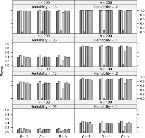
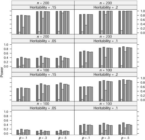
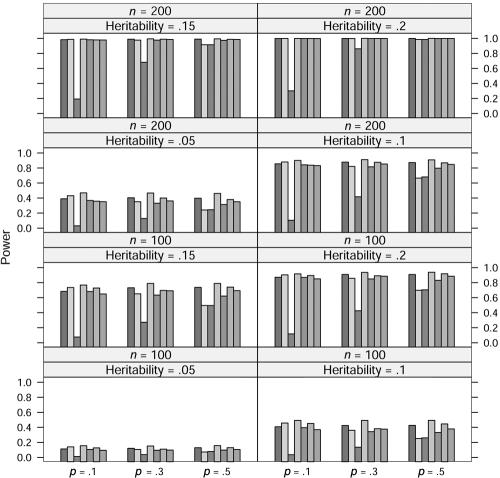
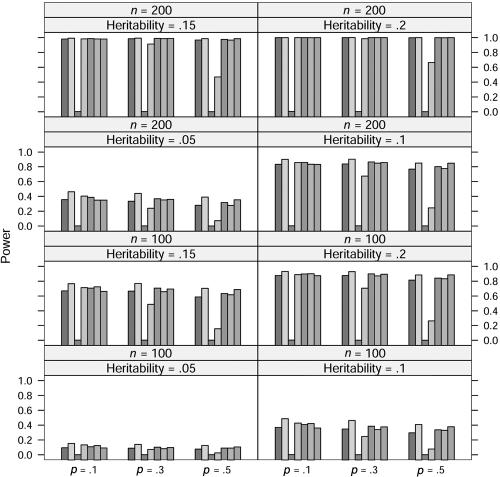
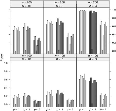
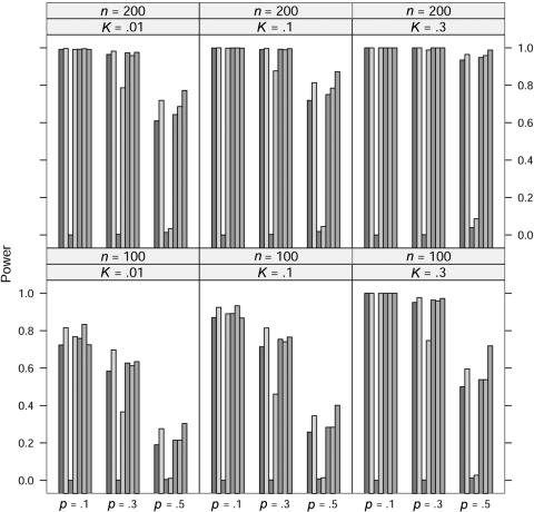
In the power study, the critical values for statistics Λ_New, Λ_Dom, Λ_Rec, Λ_Add, Λ_Larger, and Λ_Unc are from the respective asymptotic null distributions of these statistics, and the critical values for statistic Λ_Largest at allele A frequency p=0.1, 0.3, and 0.5 are obtained from a simulation with 10,000 replications. At significance level 0.001, the power of these seven statistics at allele frequency p=0.1, 0.3, and 0.5, heritability h²=0.05, 0.1, 0.15, and 0.2, and sample size n=100 and 200 is graphed in figures 1, 2, 3, and 4, in which the generating models are dominant, recessive, additive, and overdominant, respectively. It can be seen from these figures that, as expected, the statistic Λ_Dom performs best when the generating model is dominant, as do the statistic Λ_Rec when the model is recessive and the statistic Λ_Add when the model is additive. The statistic Λ_Dom performs worst when the generating model is recessive, and the statistic Λ_Rec performs worst when it is dominant. Overall, the four statistics Λ_New, Λ_Larger, Λ_Largest, and Λ_Unc seem to have similar power. When the generating model is dominant or recessive, the statistic Λ_Larger shows marginally the best power among these four statistics. When the generating model is additive, the statistic Λ_Largest is slightly better than any of the other three. For the overdominance model, the statistic Λ_New has slightly more power than the statistic Λ_Unc for p=0.1. For p=0.3 and p=0.5, the statistic Λ_Unc shows higher power than the statistic Λ_New.

Figure 1.

Power comparison for the quantitative trait when the generating model is dominant. The significance level is 0.001. The order of statistics (shaded bars) is (from left to right): Λ_New, Λ_Dom, Λ_Rec, Λ_Add, Λ_Larger, Λ_Largest, and Λ_Unc.

Figure 2.

Power comparison for the quantitative trait when the generating model is recessive. The significance level is 0.001. The order of statistics (shaded bars) is (from left to right): Λ_New, Λ_Dom, Λ_Rec, Λ_Add, Λ_Larger, Λ_Largest, and Λ_Unc.

Figure 3.

Power comparison for the quantitative trait when the generating model is additive. The significance level is 0.001. The order of statistics (shaded bars) is (from left to right): Λ_New, Λ_Dom, Λ_Rec, Λ_Add, Λ_Larger, Λ_Largest, and Λ_Unc.

Figure 4.

Power comparison for the quantitative trait when the generating model is overdominant. The significance level is 0.001. The order of statistics (shaded bars) is (from left to right): Λ_New, Λ_Dom, Λ_Rec, Λ_Add, Λ_Larger, Λ_Largest, and Λ_Unc.

Dichotomous Traits

Let be the prevalence of the trait. The frequency of genotype i would be f_ip_i/K in the cases and (1-f_i)p_i/(1-K) in the controls. In the absence of association, f₀=f₁=f₂=K, and there is no difference in genotype frequencies between cases and controls. Let γ_i=f_i/f₀, i=1,2, be the relative risk of genotype i compared with genotype 0. In the simulation, we consider a dominance model (γ₁=γ₂), a recessive model (γ₁=1), an additive model (γ₁=(1+γ₂)/2), a multiplicative model (γ₁=γ^1/2₂), and an overdominance model (γ₁=2γ₂). Given population prevalence K and the relative risk γ₂, f₀ can be determined from f₀=K/(p₀+γ₁p₁+γ₂p₂), from which f₁=γ₁f₀ and f₂=γ₂f₀ can be computed for each model. To simplify the calculation, it is assumed again that HWE holds and that the frequency of allele A is denoted by p.

The type I error rates for statistics Λ_New, Λ_Dom, Λ_Rec, Λ_Add, Λ_Larger, and Λ_Unc are reported in table 3 for allele A frequency p=0.1, 0.3, and 0.5 and sample size n=100 and 200. These results suggest that all six statistics have valid type I error rates. A similar finding is also found in simulation studies where HWE fails (data not shown).

Table 3.

Simulated Type I Error Rates for Dichotomous Traits^[Note]

	Type I Error Rate atNominal Significance Level
Frequencyof Allele A,Sample Size,and Statistic	.1	.05	.01	.001
p=.1:
n=100:
ΛNew	.0694	.0270	.0047	.0003
ΛDom	.1094	.0516	.0107	.0007
ΛRec	.1028	.0164	.0003	.0000
ΛAdd	.1041	.0522	.0112	.0008
ΛLarger	.0713	.0271	.0060	.0003
ΛUnc	.0732	.0329	.0059	.0004
n=200:
ΛNew	.1158	.0494	.0075	.0006
ΛDom	.1064	.0520	.0095	.0013
ΛRec	.2008	.0577	.0039	.0001
ΛAdd	.1045	.0531	.0106	.0011
ΛLarger	.1057	.0424	.0064	.0008
ΛUnc	.1101	.0484	.0078	.0006
p=.3:
n=100:
ΛNew	.1068	.0544	.0118	.0009
ΛDom	.0869	.0570	.0120	.0009
ΛRec	.1111	.0621	.0145	.0012
ΛAdd	.1033	.0536	.0096	.0005
ΛLarger	.1134	.0553	.0138	.0011
ΛUnc	.1103	.0580	.0119	.0013
n=200:
ΛNew	.0935	.0445	.0099	.0017
ΛDom	.1039	.0539	.0081	.0009
ΛRec	.0978	.0493	.0105	.0020
ΛAdd	.1035	.0499	.0082	.0014
ΛLarger	.0999	.0499	.0104	.0014
ΛUnc	.0971	.0480	.0113	.0016
p=.5:
n=100:
ΛNew	.0968	.0487	.0100	.0006
ΛDom	.1017	.0498	.0101	.0011
ΛRec	.1012	.0509	.0101	.0006
ΛAdd	.1014	.0492	.0106	.0007
ΛLarger	.1073	.0546	.0109	.0010
ΛUnc	.1039	.0558	.0115	.0007
n=200:
ΛNew	.0977	.0471	.0084	.0007
ΛDom	.1008	.0503	.0088	.0011
ΛRec	.1023	.0539	.0102	.0006
ΛAdd	.1053	.0525	.0103	.0009
ΛLarger	.1054	.0508	.0088	.0007
ΛUnc	.1032	.0488	.0083	.0006

Note.— Half of the sample is cases, and the other half is controls.

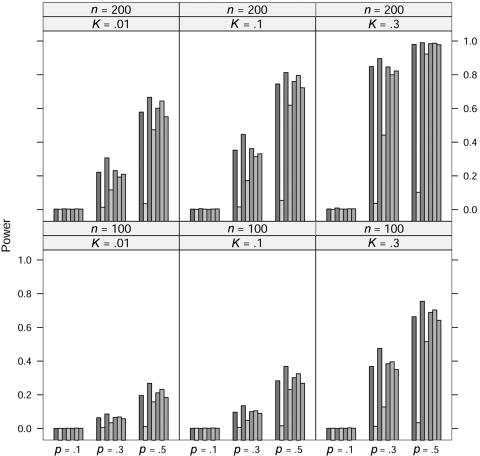
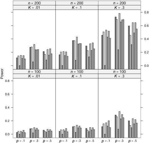
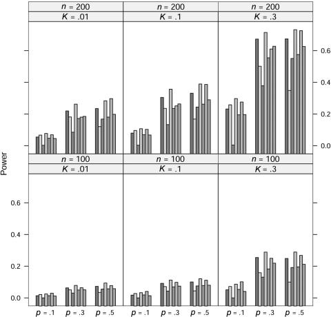
In the power study, the critical values for the seven statistics, including Λ_Largest, are obtained in the same manner as in the case of quantitative traits. At significance level 0.001, the power of the seven statistics is simulated for allele A frequency p=0.1, 0.3, and 0.5, prevalence K=0.01, 0.1, and 0.3, and sample size n=100 and 200 under five models; the results for the dominance model, the recessive model, the additive model, the multiplicative model, and the overdominance model are graphed in figures 5, 6, 7, 8, and 9, respectively. In these simulations, the value of γ₂ is fixed at γ₂=3. Similar simulations were also done for γ₂=2, but the patterns were similar and so the results are not reported here. The pattern of the power for these seven statistics is similar to that in the case of quantitative traits.

Figure 5.

Power comparison for the dichotomous trait when the generating model is dominant. The significance level is 0.001. Half of the sample is cases, and the other half is controls. The order of statistics (shaded bars) is (from left to right): Λ_New, Λ_Dom, Λ_Rec, Λ_Add, Λ_Larger, Λ_Largest, and Λ_Unc.

Figure 6.

Power comparison for the dichotomous trait when the generating model is recessive. The significance level is 0.001. Half of the sample is cases, and the other half is controls. The order of statistics (shaded bars) is (from left to right): Λ_New, Λ_Dom, Λ_Rec, Λ_Add, Λ_Larger, Λ_Largest, and Λ_Unc.

Figure 7.

Power comparison for the dichotomous trait when the generating model is additive. The significance level is 0.001. Half of the sample is cases, and the other half is controls. The order of statistics (shaded bars) is (from left to right): Λ_New, Λ_Dom, Λ_Rec, Λ_Add, Λ_Larger, Λ_Largest, and Λ_Unc.

Figure 8.

Power comparison for the dichotomous trait when the generating model is multiplicative. The significance level is 0.001. Half of the sample is cases, and the other half is controls. The order of statistics (shaded bars) is (from left to right): Λ_New, Λ_Dom, Λ_Rec, Λ_Add, Λ_Larger, Λ_Largest, and Λ_Unc.

Figure 9.

Power comparison for the dichotomous trait when the generating model is overdominant. The significance level is 0.001. Half of the sample is cases, and the other half is controls. The order of statistics (shaded bars) is (from left to right): Λ_New, Λ_Dom, Λ_Rec, Λ_Add, Λ_Larger, Λ_Largest, and Λ_Unc.

For the recessive model, these seven statistics have very similar power when allele A frequency p=0.1. We suspect that this may be caused by the rarity of the genotype homozygous for allele A, since all statistics would be close to the same likelihood-ratio statistic that tests the equality of the genotype effects between the other two genotypes.

Discussion

We have developed a constrained-likelihood approach to marker-trait association analysis. This approach does not require the specification of an analysis model. We investigated two applications of this approach, one for quantitative traits and the other for dichotomous traits. The asymptotic distribution of the constrained likelihood-ratio statistic was derived for both types of traits. Simulation studies suggest that this approach has power to detect association for a range of genetic models. Simulation results also suggest that the power of this approach seems to be close to that of the model-based method when the analysis model is correctly specified. It should be noted that the constrained-likelihood approach has been applied to linkage analyses performed using affected siblings (Holmans 1993) and using extreme discordant sib pairs (Knapp 1998; Freidlin et al. 2003) and to association studies using parent-sibs trios (Zheng et al. 2003) but not to the situation considered in the current article.

This approach provides an alternative to the model-based method and to the statistic Λ_Unc that does not have any restriction on the genotypic means. It has power for a wider range of underlying models than does the model-based method, and it is more specific than the statistic Λ_Unc. It seems to be an appealing alternative method for cases in which specification of an analysis model is inappropriate—for instance, in studies in which numerous phenotypes are analyzed simultaneously, such as expression QTL mapping (Brem et al. 2002; Schadt et al. 2003; Yvert et al. 2003; Morley et al. 2004).

This approach is related to order-restricted inference methods (Robertson et al. 1988). Order-constrained inference methods are suitable for situations in which the allele being tested for association is expected to increase or decrease the trait value—for instance, gene-mapping association studies of knockout mice. In comparison, the proposed approach does not require any ordering of the mean genotypic effects. What it requires is that the mean effect of the heterozygous genotype not exceed those of the two homozygous genotypes. In other words, if one copy of the allele being tested has an increasing or decreasing effect on the trait, then having an additional copy of this allele will not weaken this trend, regardless of its direction. That is, the allele under investigation shows no overdominance effect.

This approach provides a single-marker test. There are some recent findings that single-marker tests can be used to construct inferential procedures for haplotype analysis that are more powerful than some commonly used haplotype analysis methods (Roeder et al. 2005; Schaid et al. 2005). So, our approach has some interesting implications for haplotype analysis as well. For instance, Roeder et al. (2005) studied the performance of, among other inferential procedures, a statistic that is the largest single-marker test statistic over a set of markers. By permuting the affection status among cases and controls, it was found that this statistic is more powerful than a test proposed by Chapman et al. (2003). The single-marker test used by Roeder et al. (2005) is based on allele counts and requires HWE for it to be valid (Sasieni 1997). On the other hand, our proposed approach is based on genotypes and does not require HWE for its validity. It will be interesting to assess the performance of the procedures of Roeder et al. (2005) when the single-marker test is substituted with the test proposed here.

The constrained-likelihood approach presented here is conceptually simple. Such simplicity may be useful for its generalization to situations other than those considered here. For instance, one could include covariates in the analysis or consider markers with more than two alleles.

Appendix A : Asymptotic Distribution of Λ_New: Continuous Traits

It is straightforward to obtain that, under H₀, the Fisher information matrix for (δ₁,δ₂,α,σ²) is

According to theorem 16.7 of van der Vaart (1998), when the null hypothesis is true, the likelihood-ratio statistic Λ_New converges to

as n→∞, where X is normally distributed with mean vector 0 and covariance matrix I^-1₀.

Let be the partial variance matrix of the first two components of X, given the latter two components. That is,

After some matrix calculation, it can be shown that Γ can be written as

where is a bivariate normal random vector with mean vector 0 and variance matrix , , and . For Γ to have 2 df, the two components of must be either both strictly positive or both strictly negative. Since the correlation coefficient between these two components is γ=(p₀p₂)^1/2[(1-p₀)(1-p₂)]^-1/2, the probability that the two components are both strictly positive or both strictly negative is 2×(2π)^-1arccos(γ)=2κ. When both components of are strictly positive or negative, the constraint δ₁δ₂⩾0 is not binding and Γ has 2 df.

The probability that Γ does not have 2 df is 1-2κ. In this case, we have Λ_New=Λ_Larger=max{Λ_Dom,Λ_Rec}. According to standard asymptotic theory (e.g., that of Cox and Hinkley [1974]), Λ_Dom is asymptotically equivalent to the score statistic T²_Dom, where

and Λ_Rec is asymptotically equivalent to the score statistic T²_Rec, where

The maximum-likelihood estimate of σ² under the null hypothesis is

where is the grand mean of the trait. The correlation coefficient between T_Dom and T_Rec is (n₀n₂)^1/2[(n-n₀)(n-n₂)]^-1/2, which converges to γ=(p₀p₂)^1/2[(1-p₀)(1-p₂)]^-1/2 as n→∞. Asymptotically, T_Dom and T_Rec jointly follow bivariate normal distribution (z₁,z₂)^t, whose correlation coefficient is γ and for which both z₁ and z₂ follow the standard normal distribution. Hence, for any x⩾0, we have

Appendix B : Asymptotic Distribution of Λ_New: Dichotomous Traits

The arguments for dichotomous traits are parallel to those for continuous traits given in appendix A. For dichotomous traits, the Fisher information matrix I₀ becomes

and the matrix becomes

Both matrices are proportional to those in appendix A. So, the probability that Λ_New has 2 df remains the same.

The calculation of Λ_Larger is also parallel. The expressions for T_Dom and T_Rec remain the same, but the expression for is different. In the situation of dichotomous traits, we need to substitute with , where is the proportion of cases among the total number of subjects. This change in does not affect the asymptotic distribution of Λ_Larger or, hence, that of Λ_New.

References

- Brem RB, Yvert G, Clinton R, Kruglyak L (2002) Genetic dissection of transcriptional regulation in budding yeast. Science 296:752–755 10.1126/science.1069516 [DOI] [PubMed] [Google Scholar]
- Chapman JM, Cooper JD, Todd JA, Clayton DG (2003) Detecting disease associations due to linkage disequilibrium using haplotype tags: a class of tests and the determinants of statistical power. Hum Hered 56:18–31 10.1159/000073729 [DOI] [PubMed] [Google Scholar]
- Cox DR, Hinkley DV (1974) Theoretical statistics. Chapman and Hall, London [Google Scholar]
- Falconer DS, Mackay TFC (1996) Introduction to quantitative genetics, 4th ed. Prentice Hall, London [Google Scholar]
- Freidlin B, Zheng G, Li Z, Gastwirth J (2002) Trend tests for case-control studies of genetic markers: power, sample size and robustness. Hum Hered 53:146–152 10.1159/000064976 [DOI] [PubMed] [Google Scholar]
- ——— (2003) Efficiency robust tests for mapping quantitative trait loci using extremely discordant sib pairs. Hum Hered 55:117–124 10.1159/000072316 [DOI] [PubMed] [Google Scholar]
- Holmans P (1993) Asymptotic properties of affected–sib-pair linkage analysis. Am J Hum Genet 52:362–374 [PMC free article] [PubMed] [Google Scholar]
- Knapp M (1998) Evaluation of a restricted likelihood ratio test for mapping quantitative trait loci with extreme discordant sib pairs. Ann Hum Genet 62:75–87 10.1017/S0003480098006617 [DOI] [PubMed] [Google Scholar]
- Morley M, Molony CM, Weber TM, Devlin JL, Ewens KG, Spielman R, Cheung VG (2004) Genetic analysis of genome-wide variation in human gene expression. Nature 430:733–734 10.1038/430733a [DOI] [PMC free article] [PubMed] [Google Scholar]
- Prentice RL, Pyke R (1979) Logistic disease incidence models and case-control studies. Biometrika 66:403–411 [Google Scholar]
- Robertson T, Wright FT, Dykstra RL (1988) Order restricted statistical inference. John Wiley & Sons, New York [Google Scholar]
- Roeder K, Bacanu SA, Zhao X, Devlin B (2005) Analysis of single-locus tests to detect gene/disease associations. Genet Epidemiol 28:207–219 10.1002/gepi.20050 [DOI] [PubMed] [Google Scholar]
- Sasieni PD (1997) From genotypes to genes: doubling the sample size. Biometrics 53:1253–1261 [PubMed] [Google Scholar]
- Schadt EE, Monks SA, Drake TA, Lusis AJ, Che N, Colinayo V, Ruff TG, Milligan SB, Lamb JR, Cavet G, Linsley PS, Mao M, Stoughton RB, Friend SH (2003) Genetics of gene expression surveyed in maize, mouse and man. Nature 422:297–302 10.1038/nature01434 [DOI] [PubMed] [Google Scholar]
- Schaid DJ, McDonnell SK, Hebbring SJ, Cunningham JM, Thibodeau SN (2005) Nonparametric tests of association of multiple genes with human disease. Am J Hum Genet 76:780–793 [DOI] [PMC free article] [PubMed] [Google Scholar]
- Slager S, Schaid D (2001) Case-control studies of genetic markers: power and sample size approximations for Armitage’s test for trend. Hum Hered 52:149–153 10.1159/000053370 [DOI] [PubMed] [Google Scholar]
- van der Vaart AW (1998) Asymptotic statistics. Cambridge University Press, Cambridge [Google Scholar]
- Yvert G, Brem RB, Whittle J, Akey JM, Foss E, Smith EN, Mackelprang R, Kruglyak L (2003) Trans-acting regulatory variation in Saccharomyces cerevisiae and the role of transcription factors. Nat Genet 35:57–64 10.1038/ng1222 [DOI] [PubMed] [Google Scholar]
- Zheng G (2003) Use of max and min scores for trend tests for association when the genetic model is unknown. Stat Med 22:2657–2666 10.1002/sim.1474 [DOI] [PubMed] [Google Scholar]
- Zheng G, Chen Z, Li Z (2003) Tests for candidate-gene association using case-parents design. Ann Hum Genet 67:589–597 10.1046/j.1529-8817.2003.00065.x [DOI] [PubMed] [Google Scholar]