

Abstract
Mutation of the human genome ranges from single base-pair changes to whole-chromosome aneuploidy. Karyotyping, fluorescence in situ hybridization, and comparative genome hybridization are currently used to detect chromosome abnormalities of clinical significance. These methods, although powerful, suffer from limitations in speed, ease of use, and resolution, and they do not detect copy-neutral chromosomal aberrations—for example, uniparental disomy (UPD). We have developed a high-throughput approach for assessment of DNA copy-number changes, through use of high-density synthetic oligonucleotide arrays containing 116,204 single-nucleotide polymorphisms, spaced at an average distance of 23.6 kb across the genome. Using this approach, we analyzed samples that failed conventional karyotypic analysis, and we detected amplifications and deletions across a wide range of sizes (1.3–145.9 Mb), identified chromosomes containing anonymous chromatin, and used genotype data to determine the molecular origin of two cases of UPD. Furthermore, our data provided independent confirmation for a case that had been misinterpreted by karyotype analysis. The high resolution of our approach provides more-precise breakpoint mapping, which allows subtle phenotypic heterogeneity to be distinguished at a molecular level. The accurate genotype information provided on these arrays enables the identification of copy-neutral loss-of-heterozygosity events, and the minimal requirement of DNA (250 ng per array) allows rapid analysis of samples without the need for cell culture. This technology overcomes many limitations currently encountered in routine clinical diagnostic laboratories tasked with accurate and rapid diagnosis of chromosomal abnormalities.
Introduction
Chromosome abnormalities are associated with a wide range of clinical problems, from cancer to abnormal morphological and neurological development in neonates, children, and adolescents. The identification and characterization of chromosome abnormalities represent the cornerstone of cytogenetic analysis and are crucial for the accurate diagnosis and prognosis of associated clinical disorders. Current methods used for assessing chromosomal integrity and copy number focus on microscopy of metaphase chromosome spreads and interphase nuclear preparations; these techniques include karyotyping and FISH. Despite the great diagnostic and prognostic benefits provided by these methods, microscopy has several obvious shortcomings. First, resolution is limited to large amplifications, deletions, and translocations of 3–5 Mb and greater. Second, preparation of chromosome spreads requires cell cultures, which can take several weeks, and is often unsuccessful in biopsy samples from patients with cancer (Mandahl 1992). The ever-increasing catalogue of microdeletions and duplications associated with specific single-gene disorders and clinical syndromes indicates that there is a complete spectrum of copy-number mutation sizes, with a range from very large to potentially very small (Sellner and Taylor 2004). Other comparative genomic hybridization (CGH) approaches to genomewide detection of copy-number changes use a large number of discrete genomic or cDNA clones in arrays (array-based CGH) (Kallioniemi et al. 1992; Albertson et al. 2000; Hodgson et al. 2001; Snijders et al. 2001; Pollack et al. 2002; Ishkanian et al. 2004). Several limitations of these CGH arrays include the need for large amounts of starting material, resolution limited by the number of clones that can be deposited on the arrays, reagent variability from site to site, and lack of manufacturing standards; all of these constraints make it difficult for individual laboratories to conduct reproducible experiments. Therefore, an easy, rapid, and robust technology capable of identifying genomewide aberrations at ultrahigh resolution would represent an important advance in clinical diagnostics.
High-density synthetic oligonucleotide microarrays have been developed for the ability to access large quantities of genetic information in a single experiment (Fodor et al. 1991, 1993; Pease et al. 1994). These arrays have been used extensively to measure RNA transcripts (reviewed by Kapranov et al. [2003]), to resequence DNA (Warrington et al. 2002), and to accurately genotype thousands of SNPs (Kennedy et al. 2003), all with use of simple biochemical target preparation methods and minimal instrumentation.
The principle of using high-density SNP genotyping arrays for DNA copy-number analysis has been demonstrated elsewhere, first with arrays containing 1,494 SNPs and, subsequently, with arrays containing 11,555 SNPs. The majority of these studies have focused on cancers (Lindblad-Toh et al. 2000; Primdahl et al. 2002; Schubert et al. 2002; Dumur et al. 2003; Hoque et al. 2003; Lieberfarb et al. 2003; Bignell et al. 2004; Huang et al. 2004; Janne et al. 2004; Paez et al. 2004; Wang et al. 2004; Wong et al. 2004; Zhou et al. 2004a, 2004b), but a recent report used microarrays with 11,555 SNPs to study constitutional copy-number changes in mentally retarded individuals (Rauch et al. 2004). Such arrays not only provide SNP genotypes at >99.5% accuracy, but they also utilize quantitative hybridization signal intensities to estimate copy-number changes, such as amplifications and deletions (Bignell et al. 2004; Huang et al. 2004). In addition, the approach of combining genotypes and copy-number estimation allows the detection of regions of loss of heterozygosity (LOH) with or without copy-number change (Zhao et al. 2004).
Rapid advances in high-density SNP genotyping technology have resulted in the recent development of commercially available arrays, Affymetrix GeneChip 100K mapping arrays, that contain 116,204 genomewide SNPs (Matsuzaki et al. 2004b). The mean and median inter-SNP distances of this set are 23.6 kb and 8.5 kb, respectively. Over 99% of the genome is within 500 kb of a SNP (i.e., 0.5 Mb), and 91% of the genome is within 100 kb of a SNP (Matsuzaki et al. 2004a); this provides the capability of assessing copy-number changes at an unprecedented resolution. The 100K mapping array selects against SNPs in segmental duplications because it selects SNPs on the basis of genotyping accuracy, robustness, Mendelian inheritance, Hardy-Weinberg equilibrium, duplicates, and reproducibility (H. Matsuzaki, personal communication).
Here, we describe the application of 100K mapping arrays for detection of clinically significant cytogenetic abnormalities, both constitutional and acquired. Notably, the resolution of these arrays permits detection of submicroscopic copy-number abnormalities.
Material and Methods
Clinical Cases
All clinical cases were referred for routine cytogenetic analysis—by obstetric, pediatric, or neurology specialists—by use of stored DNA. The study complied with internal ethics committee requirements. Our sample population consisted of 23 individuals, 17 with known cytogenetic abnormalities, including unbalanced, structural, and whole-chromosome abnormalities (table 1). The raw genotypes for all patients in this study are included in a tab-delimited ASCII file (online only) that can be imported into a spreadsheet. In some cases, characterization was incomplete because of the limitations of conventional analysis or lack of patient material.
Table 1.
Summary of Patient Data
|
Alterations Identified by Conventional Cytogenetics |
|||||||
| Chromosomal Abnormality,Patient, and SNP Intervala | No. of SNPs | Size(Mb) | Physical Location | Specific Related Disorder | Abnormal Karyotypeb | Identification Methodc | EstimatedSized(Mb) |
| Deletion: | |||||||
| A1: | |||||||
| SNP_A-1685059–SNP_A-1656379 | 510 | 13.6 | Chromosome 12:97665490–111224235 | … | del(12)(q23.1q24.13) | Karyotype | ND |
| A2: | |||||||
| SNP_A-1653255–SNP_A-1747962 | 95 | 1.3 | Chromosome 17:14374914–15681675 | HNPP | del(17)(p11.2p11.2) | MLPA | 1.3 |
| A3: | |||||||
| SNP_A-1651282–SNP_A-1686492 | 139 | 5.3 | Chromosome 15:20551112–25877344 | PWS | del(15)(q12q12) | Karyotype/MS-PCR | ND |
| A4: | |||||||
| SNP_A-1734992–SNP_A-1642272 | 38 | 1.6 | Chromosome 15:21851887–23392190 | AS | del(15)(q12q12) | FISH (SNRPN exon1) | ND |
| SNP_A-1652025–SNP_A-1644720 | 64 | 1.7 | Chromosome 15:23975849–25703496 | ||||
| A5e: | |||||||
| SNP_A-1727145–SNP_A-1718251 | 329 | 7.1 | Chromosome 5:83044807–90111353 | … | del(5)(q14.2q15) | RP11-662G5 and RP11-158N5 | 6.9 |
| A6: | |||||||
| SNP_A-1737080–SNP_A-1748287 | 433 | 8.9 | Chromosome 5:82289925–91227139 | … | del(5)(q14.2q15) | RP11-605H18 and RP11-68F17 | 8.6 |
| A7e: | |||||||
| SNP_A-1642645–SNP_A-1726825 | 263 | 6.2 | Chromosome 5:88641401–94876462 | … | del(5)(q14.2q15) | RP11-276J11 and RP11-626H3 | 6.3 |
| A8e: | |||||||
| SNP_A-1680648–SNP_A-1746773 | 213 | 4.6 | Chromosome 17:9583769–14214760 | … | del(17)(p12p13.1) | RP11-20O2 and RP11-601N13 | 4.9 |
| Duplication: | |||||||
| B1: | |||||||
| SNP_A-1683609–SNP_A-1671009 | 97 | 1.4 | Chromosome 17:14181216–15583354 | CMT1A | dup(17)(p11.2p11.2) | MLPA, FISH | 1.3 |
| B2: | |||||||
| SNP_A-1675179–SNP_A-1730712 | 59 | 2.5 | Chromosome X:134373326–136865347 | X-linked hypothyroidism | dup(X)(q26q27) | RP11-432N13 | 7.7 |
| SNP_A-1734959–SNP_A-1734676 | 95 | 2.8 | Chromosome X:137966285–140795635 | dup(X)(q26q27) | GS1-91O18 | ||
| B3e: | |||||||
| SNP_A-1663401–SNP_A-1656284 | 255 | 7.4 | Chromosome 16:46777645–54135758 | … | dup(16)(q12.1q12.2) | RP11-91A22 and RP11-1061C23 | 7.9 |
| B4: | |||||||
| SNP_A-1691939–SNP_A-1737935 | 397 | 7.7 | Chromosome 6:99536–7800082 | … | dup(6)(p25p25) | MLPA (IRF4), WCP-6 (whole chromosome 6 paint) | ND |
| Aneuploidy and/or others: | |||||||
| C1: | |||||||
| SNP_A-1712184–SNP_A-1726775 | 2,776 | 56.3 | Chromosome 11:77932282–134206317 | ALL | del(11)(q23qter) | Karyotype | ND |
| SNP_A-1759012–SNP_A-1665643 | 112 | 1.5 | Chromosome 7:36579196–38108039 | del(7)(p14.1p14.2) | Previously unidentified | ND | |
| SNP_A-1680920–SNP_A-1642739 | 558 | 30.0 | Chromosome X:123443585–153277935 | dup(X)(q25q28) | Previously unidentified | ND | |
| C2e: | |||||||
| Not detected | … | … | … | del(9)(q34.3) | MLPA (MRPL41) | ND | |
| SNP_A-1718890–SNP_A-1682693 | 135 | 7.0 | Chromosome 1:2103664–9141936 | dup(1)(p36.22) | MLPA (CAB45) | ND | |
| C3: | |||||||
| SNP_A-1650041–SNP_A-1691107 | 563 | 4.8 | Chromosome 8:2091837–6895465 | … | del(8)(p23.1) | MLPA (FBXO25) | ND |
| SNP_A-1691210–SNP_A-1684761 | 47 | 11.0 | Chromosome 19:341341–11295505 | dup(19)(p13.2p13.3) | MLPA (CDC34) | ND | |
| C4: | |||||||
| SNP_A-1752387–SNP_A-1695260 | 6,975 | 145.9 | Chromosome 8:180568–146086167 | Trisomy 8 | 48,XX,+8,+21 | Karyotype | ND |
| SNP_A-1654532–SNP_A-1755352 | 1,913 | 37.0 | Chromosome 21:9929029–46956357 | Trisomy 21 | 48,XX,+8,+21 | Karyotype | ND |
| C5: | |||||||
| SNP_A-1654532–SNP_A-1755352 | 1,913 | 37.0 | Chromosome 21:9929029–46956357 | Trisomy 21 | 47,XX,t(12;21)(q12;p13),+21 | Karyotype | ND |
The SNP ID for the start and end of the regions, the number of SNPs located within the regions, and the size and physical location (NCBI version 34, July 2003) are indicated for each sample, as determined by the GeneChip 100K mapping arrays.
Karyotypes were determined by standard cytogenetic banding. These analyses allowed classification of the chromosomal aberration as a deletion (del), duplication (dup), or other rearrangements with or without aneuploidy.
Samples were independently verified by either karyotyping, FISH analysis with use of BAC probes (BACs at each end of the abnormality are listed), MLPA, or methylation-sensitive PCR (MS-PCR).
Determined by mapping through use of FISH or MLPA. ND=not determined.
Samples that were done in duplicate.
100K Mapping Arrays
The Mapping 100K Set comprises two arrays (one uses XbaI, and the other, HindIII restriction enzymes), each with >50,000 SNPs (XbaI has 58,960 SNPs, and HindIII has 57,244 SNPs, for a total of 116,204 SNPs). The spacing of the SNPs on these arrays indicates that 99.1% of the genome is within 500 kb of a SNP, 91.6% is within 100 kb, and 40% is within 10 kb (Matsuzaki et al. 2004a). These calculations exclude centromeres, telomeres, and heterochromatin, which account for 0.226 Gb (total genome size=3.069 Gb; after removal of these large gaps, the effective genome size=2.843 Gb). The largest span between SNPs (4.9 Mb) is on the X chromosome.
Data Analysis
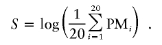
Genotype calls were determined using GeneChip DNA Analysis software (GDAS). Copy-number estimations were determined using the CHP file output from GDAS and GeneChip Chromosome Copy Number Analysis Tool (CNAT), which is available, free of charge, for download at the Affymetrix Web site. CNAT implements an algorithm that uses genotype information and signal-probe intensities to calculate copy-number changes that are based on SNP hybridization signal-intensity data from the experimental sample relative to intensity distributions derived from a set of 100 normal reference individuals (Huang et al. 2004). The log of the arithmetic average of the perfect match (PM) intensities across 20 probes (S) is used as the basic measurement for any given SNP.
 |
After S is calculated, it is scaled to have a mean of 0 and a variance of 1 for all autosomal SNPs, to decrease the variability across samples. Sample normalization is done across all features on the array,
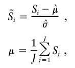 |
and
 |
where J is the number of SNPs.
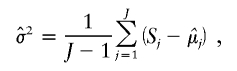
To determine the significance of a copy-number change for a specific SNP, the signal-intensity variation of the SNP across a set of normal samples is determined. The statistics are calculated for each genotype of SNP, with allowance for genotype dependencies in the statistics. The mean and variance are estimated across the normal samples,
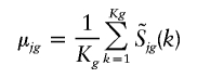 |
and
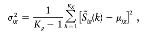 |
where k=1,…Kg are the normal samples with the same genotype, g=(AA,BB,AB). The normalized intensity for the SNP is compared with the expected intensity for CN=2, as determined by the log intensity of the SNP in the reference set, with use of the copy-number (CN) response curve determined from dosage response data,
where a=0.658 and b=0.714 for Mapping 50K XbaI and a=0.638 and b=0.703 for Mapping 50K HindIII. This corresponds to the single-point-analysis copy number (SPA_CN). The significance of the copy-number variation (CNV) is estimated by comparison with the reference set. For each SNP, separate statistics are derived for each genotype in the reference set,
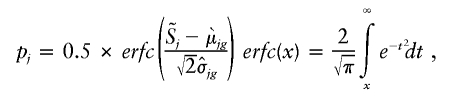 |
so comparisons are made with samples sharing the same genotype, for calculation of the probability that CN=2, known as the P value. We report the −log P value. The larger the number, the less probable that the copy number is equal to 2. If −log P is very large, then it is very unlikely that CN=2. A Gaussian kernel-smoothing average was also used for averaging the copy number and P value of individual SNPs over a fixed genomic interval. The smoothing averages out the random noise across neighboring SNPs and minimizes the false-positive rate (FPR), while keeping the true-positive rate high. The kernel-smoothing accentuates genomic intervals in which consecutive SNPs display the same type of alteration (gain or loss). The default window size of 0.5 Mb was used, unless otherwise indicated.
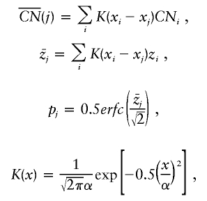 |
and
In general, when analyzing an unknown sample, the recommended approach is to use the default window size of 0.5 Mb, because of the spacing of the SNPs on these arrays (99.1% of the genome is within 0.5 Mb). After review of the initial data, a larger window may be appropriate, if the detected aberration is significantly larger than the default window size. By increasing the window size, the noise is reduced because of incorporation of many more adjacent probes into the window. This is advantageous only if all of the probes in the window are expected to behave the same; that is, they have undergone the same aberration, such as a whole-chromosome trisomy. It should be noted that a trisomy can be detected using either the default window size or a larger window size; the major difference is in the confidence (P value) associated with the trisomy. Both the copy number and P values are smoothed. These smooth copy number and P values are referred to as “GSA_CN” and “GSA_pVal,” respectively.
The LOH score calculates the probability of being homozygous for each SNP from the reference file. If each SNP is treated independently, then the probability of a stretch of SNPs (position m→n) all being homozygous can be calculated.
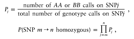 |
and
Regions of duplication and deletion are reported as the first and last SNP showing either (1) significant increases in copy number associated with a positive P value or (2) decreased copy number, negative P value, and associated LOH (table 1).
Original Identification and Verification Methods
FISH with use of BACs was performed on interphase or metaphase chromosome preparations by standard methods (Lichter and Cremer 1992). Multiplex ligation-dependent probe amplification (MLPA) assays were obtained from MRC-Holland. The MLPA protocol has been described in detail elsewhere (Schouten et al. 2002). Quantitative genomic real-time PCR was performed as a duplex PCR for the test exons labeled with FAM and CFTR exon 24 (MIM 602421), used as an internal control and labeled with HEX. The HEX-labeled undeleted control was also run as a duplex PCR with FAM-labeled exons 2 and 5 from the APC gene (MIM 175100). The TaqMan fluorescent probes were synthesized in accordance with the Applied Biosystems primer express software program. The PCR protocol with use of the Platinum QPCR mix was performed in accordance with the manufacturer’s instructions (Invitrogen). The Ct (threshold cycle) value of the test probe and control probe are compared and normalized using the 2-(2ΔCt) method (Applied Biosystems), where ΔCt is the difference between the test and the control and 2ΔCt is the difference between the ΔCt value and the average ΔCt of the normal control samples. A final “normalized value,” 2-(2ΔCt), of <0.5 is indicative of a deletion.
Results
We tested cases containing heterozygous deletions, duplications, whole-chromosome aneuploidy, other unbalanced rearrangements, and uniparental disomy (UPD) (table 1). Most of these cases have been partly or fully characterized elsewhere, with use of other techniques, such as FISH and MLPA-PCR (Slater et al. 2003; Rooms et al. 2004). In all cases, the physical position of each deletion or duplication determined by SNP analysis was consistent with the karyotype band location.
Analysis of Problematic Samples
Karyotyping suffers from the limitations of chromosome banding, sample preparation, and subjective analysis. Common causes of unsuccessful or inaccurate cytogenetic testing are suboptimal quality of metaphase preparations, inability to stimulate cell division in culture (particularly troublesome in the testing of leukemic bone marrows from children and necrotic products of conception), and samples that contain inadequate numbers of viable cells for processing.
Patient C1, a female with pediatric acute lymphocytic leukemia (ALL), exemplifies several of the main advantages of using the Mapping 100K approach for problematic samples. Bone marrow G-banded chromosome preparations from this type of sample are typically very poor and consequently allow, at best, only low-resolution (i.e., <400 bands) analysis. A complex karyotype involving two abnormal clones—46,XX,del(11)(q23)[2]/45,X,-X,del(11)(q23),inc[5]/46,XX[5]—was initially observed. Of 300 cells analyzed using FISH, 81% showed an apparent deletion of chromosome 11 at band q23, which is clinically relevant because of the potential involvement of the mixed-lineage leukemia gene (MLL [MIM 159555]). Many cells contained only one X chromosome; other abnormalities were suspected, but none was clearly identifiable. The Mapping 100K arrays showed a large 56.3-Mb terminal deletion of chromosome 11 at band q14.3 and a 30-Mb duplication of chromosome X at band Xq25 (table 1). The array data indicated that the breakpoint was at 11q14.3 rather than 11q23, which demonstrates that higher-resolution analysis allows for more-accurate breakpoint determinations (see below). Together with the Mapping 100K data, reinterpretation of the karyotype is consistent with a derivative that consists of chromosome 11 with a breakpoint at q14.3 ligated to the distal region of Xq25-ter. In addition, a small (1.5 Mb) deletion was found on chromosome 7 at band p14.1-14.2, which is one of the smallest deletions observed in the present study (fig. 1) and was not detected in the original analysis (table 1). We verified this deletion, using quantitative real-time PCR with two different sequences selected from exons located within the deleted region, as well as control sequences located outside the deleted region (table 2). Patient C1 and four unaffected control samples were assayed twice in triplicate. For probes within the deleted region, the normalized values for patient C1 were <0.5 (0.21 and 0.23 for BC039725 and ELMO1, respectively), which indicates a deletion. For probes outside the deleted region, the normalized values for patient C1 were equal to 1.18 and 0.84 for APC exons 5 and 2, respectively (table 3), which indicates no deletion. These quantitative PCR results confirm the small deletion first detected by GeneChip Mapping 100K arrays (fig. 1).
Figure 1.

Analysis of Mapping 100K data with use of CNAT. Patient C1 is shown, with the 1.5-Mb deleted region on chromosome 7p14.1-14.2 indicated by vertical lines. Chromosomal position (in Mb) is indicated on the X-axis for all three panels. Estimated copy-number changes are shown in the upper panel, P values are shown in the middle panel, and the LOH score is shown on the bottom panel. The default window size of 0.5 Mb was used.
Table 2.
Summary of Quantitative Fluorescence PCR[Note]
|
Test Probe Duplex |
Control Probe Duplex |
|||||||||||
| BC039725/CFTR Exon 24 |
Elmo1/CFTR Exon 24 |
APC Exon 5/CFTR Exon 24 |
APC Exon 2/CFTR Exon 24 |
|||||||||
| DNA Source | AveΔCT | Ave2ΔCT | 2-(2ΔCt) | AveΔCT | Ave2ΔCT | 2-(2ΔCt) | AveΔCT | Ave2ΔCT | 2-(2ΔCt) | AveΔCT | Ave2ΔCT | 2-(2ΔCt) |
| Cases (n=16) | 1.159 | 1.709 | .209 | 2.709 | 2.119 | .23 | .1 | −.242 | 1.182 | .267 | .259 | .836 |
| Controls (n=4) | −.55 | … | … | .59 | … | … | .342 | … | … | .008 | … | … |
Note.— The symbols are explained in the “Material and Methods” section.
Table 3.
Summary of Family Data on Chromosome 15[Note]
|
Genotype Concordanceon Chromosome 15(%) |
|||
| Family, Specific Related Disorder,and SNP Interval | No. of SNPs | Child vs. Mother | Child vs. Father |
| F1: | |||
| Maternal uniparental isodisomy 15: | |||
| SNP_A-1713638–SNP_A-1708745 | 87 | 72.8 | 62.2 |
| SNP_A-1753891–SNP_A-1715425 | 2,945 | 100 | 64 |
| SNP_A-1713638–SNP_A-1715425 | 3,032 | 99.2 | 64.0 |
| F2: | |||
| Maternal uniparental heterodisomy 15: | |||
| SNP_A-1713638–SNP_A-1715425 | 3,032 | 100 | 63.6 |
Note.— SNP and concordance information was determined by the GeneChip 100K mapping arrays. The 46,XY,upd(15)mat alteration was identified by microsatellites.
Patient A1 contains a derivative of a maternal insertion, ins(6;12)(p21.3;q22q23). There is an interstitial deletion on chromosome 12 involving bands q22 and q23 that was not detected in the original prenatal, 400-band, G-banded metaphase preparations. A neonatal preparation was required to identify the abnormality in 600–800 band preparations. The Mapping 100K array approach detected a 13.6-Mb deletion (table 1). The region contains ∼111 genes, including phenylalanine hydroxylase (PAH [MIM 261600]). Interestingly, this patient exhibited a low-level increase in serum phenylalanine, consistent with a single-copy deletion of PAH.
It should be noted that figure 1 also shows P values similar to the known observed deletion. Since this study was designed to determine whether the technology could detect known copy-number changes in cytogenetic referral samples, cutoffs for significance of novel abnormalities were not determined. Without extensive validation of cutoffs for significance, we cannot assess a priori whether these P values represent false-positive or true-positive results. As an initial attempt to evaluate this observed variation, we assumed that the bulk of the data in any particular sample should follow the normal distribution of a copy number equal to 2 and a P value equal to 0. In fact, the average copy number was 2.09, and the P value was 0.20 for the patients in this study (tables 4 and 5), which indicates an overall excellent fit with these expected values. In addition, we hypothesized that SNPs that fell outside the 95% CI should represent true aberrations, since they are statistically different from the overall “normal” distribution. For each of the aberrations described in table 1, we determined whether these regions fell outside the 95% CI (tables 6 and 7). Under this assumption, we determined the FPR to be 2.04%–3.48% (see appendix A).
Table 4.
Five-Value Summary of Patient Data[Note]
| GSA_CN |
GSA_pVal |
SD |
||||||||||
| Patient | Minimum | Lower Quartile | Median | Upper Quartile | Maximum | Minimum | Lower Quartile | Median | Upper Quartile | Maximum | GSA_CN | GSA_pVal |
| A1 | .00 | 1.94 | 2.06 | 2.21 | 8.30 | −20.00 | −.40 | .09 | .33 | 10.68 | .31 | 1.01 |
| A2 | .00 | 1.80 | 2.08 | 2.51 | 22.09 | −16.01 | −1.51 | .22 | 1.41 | 20.00 | .68 | 2.67 |
| A3 | .00 | 1.93 | 2.12 | 2.34 | 9.57 | −16.26 | −.70 | .26 | .82 | 20.00 | .38 | 1.45 |
| A4 | .00 | 1.98 | 2.20 | 2.49 | 24.77 | −20.00 | −.31 | .55 | 1.45 | 20.00 | .54 | 2.01 |
| A5 | .00 | 1.94 | 2.08 | 2.26 | 12.61 | −15.21 | −.45 | .14 | .45 | 20.00 | .35 | 1.23 |
| A6 | .00 | 1.91 | 2.06 | 2.24 | 8.30 | −13.57 | −.52 | .10 | .39 | 20.00 | .34 | 1.10 |
| A7 | .00 | 1.93 | 2.09 | 2.27 | 7.54 | −15.95 | −.58 | .16 | .56 | 20.00 | .35 | 1.20 |
| A8 | .00 | 1.94 | 2.07 | 2.23 | 8.62 | −8.11 | −.45 | .11 | .38 | 20.00 | .30 | .68 |
| B1 | .00 | 2.02 | 2.18 | 2.35 | 10.96 | −20.00 | .04 | .46 | 1.07 | 20.00 | .35 | 1.50 |
| B2 | .00 | 1.87 | 2.08 | 2.34 | 7.87 | −20.00 | −.91 | .16 | .77 | 20.00 | .42 | 1.54 |
| B3 | .00 | 1.92 | 2.06 | 2.22 | 7.42 | −8.11 | −.48 | .09 | .36 | 10.71 | .30 | .69 |
| B4 | .00 | 2.01 | 2.15 | 2.29 | 7.98 | −20.00 | .02 | .35 | .82 | 20.00 | .30 | 1.08 |
| C1 | .00 | 1.97 | 2.13 | 2.32 | 7.57 | −20.00 | −.39 | .29 | .78 | 20.00 | .36 | 1.34 |
| C2 | .00 | 1.96 | 2.07 | 2.21 | 6.09 | −15.65 | −.36 | .11 | .36 | 20.00 | .27 | .64 |
| C3 | .00 | 1.95 | 2.06 | 2.20 | 8.93 | −20.00 | −.35 | .09 | .31 | 20.00 | .30 | .98 |
| C4 | .00 | 1.84 | 2.04 | 2.32 | 6.49 | −11.19 | −.89 | .07 | .62 | 20.00 | .43 | 1.40 |
| C5 | .00 | 1.91 | 2.05 | 2.22 | 6.73 | −20.00 | −.54 | .08 | .39 | 20.00 | .34 | 1.14 |
| Average | .00 | 1.93 | 2.09 | 2.30 | 10.11 | −16.47 | −.52 | .20 | .66 | 18.91 | .37 | 1.27 |
Table 5.
Five-Value Summary of 42 White Reference Samples[Note]
| GSA_CN |
GSA_pVal |
SD |
||||||||||
| White Reference Sample | Minimum | Lower Quartile | Median | Upper Quartile | Maximum | Minimum | Lower Quartile | Median | Upper Quartile | Maximum | GSA_CN | GSA_pVal |
| NA17201 | .00 | 1.99 | 2.06 | 2.13 | 3.55 | −20.00 | −.09 | .07 | .18 | 2.18 | .23 | .83 |
| NA17202 | .00 | 2.00 | 2.06 | 2.12 | 4.30 | −4.45 | −.03 | .06 | .16 | 2.72 | .19 | .22 |
| NA17203 | .00 | 1.99 | 2.06 | 2.13 | 3.95 | −20.00 | −.07 | .06 | .16 | 3.24 | .23 | .87 |
| NA17204 | .00 | 1.99 | 2.05 | 2.13 | 3.53 | −2.60 | −.09 | .06 | .17 | 2.64 | .20 | .25 |
| NA17205 | .00 | 1.99 | 2.05 | 2.12 | 4.32 | −20.00 | −.08 | .08 | .22 | 6.25 | .24 | .90 |
| NA17206 | .00 | 2.00 | 2.05 | 2.11 | 3.50 | −1.93 | −.04 | .06 | .15 | 6.37 | .20 | .29 |
| NA17207 | .00 | 1.99 | 2.06 | 2.12 | 4.30 | −20.00 | −.07 | .07 | .20 | 6.21 | .23 | .89 |
| NA17208 | .00 | 2.00 | 2.06 | 2.12 | 5.10 | −2.70 | −.01 | .06 | .16 | 7.22 | .19 | .22 |
| NA17210 | .00 | 1.99 | 2.06 | 2.12 | 4.10 | −3.14 | −.05 | .07 | .17 | 1.92 | .19 | .23 |
| NA17211 | .00 | 1.99 | 2.06 | 2.14 | 4.63 | −20.00 | −.09 | .08 | .20 | 2.42 | .23 | .76 |
| NA17212 | .00 | 2.00 | 2.06 | 2.12 | 3.13 | −20.00 | −.03 | .06 | .15 | 2.84 | .23 | .77 |
| NA17213 | .00 | 2.04 | 2.14 | 2.26 | 8.63 | −20.00 | .05 | .24 | .55 | 20.00 | .27 | .69 |
| NA17214 | .00 | 1.98 | 2.07 | 2.15 | 3.68 | −20.00 | −.17 | .08 | .22 | 3.95 | .25 | .91 |
| NA17215 | .00 | 1.99 | 2.07 | 2.14 | 3.24 | −5.87 | −.06 | .07 | .18 | 3.09 | .20 | .25 |
| NA17216 | .00 | 1.99 | 2.07 | 2.14 | 4.12 | −20.00 | −.08 | .07 | .17 | 2.57 | .20 | .26 |
| NA17217 | .00 | 1.98 | 2.07 | 2.15 | 3.76 | −4.32 | −.13 | .08 | .21 | 6.63 | .21 | .28 |
| NA17220 | .00 | 2.00 | 2.05 | 2.12 | 3.77 | −20.00 | −.05 | .06 | .16 | 3.47 | .23 | .87 |
| NA17221 | .00 | 2.00 | 2.07 | 2.13 | 3.69 | −7.73 | .00 | .09 | .22 | 5.91 | .20 | .30 |
| NA17228 | .00 | 1.99 | 2.05 | 2.11 | 4.44 | −20.00 | −.05 | .06 | .15 | 2.09 | .23 | .81 |
| NA17235 | .00 | 1.99 | 2.06 | 2.12 | 5.24 | −20.00 | −.06 | .06 | .15 | 3.25 | .23 | .83 |
| NA17245 | .00 | 1.99 | 2.07 | 2.15 | 4.13 | −3.19 | −.07 | .08 | .18 | 4.92 | .20 | .27 |
| NA17247 | .00 | 1.99 | 2.05 | 2.12 | 4.72 | −2.37 | −.08 | .06 | .16 | 7.60 | .20 | .24 |
| NA17251 | .00 | 2.00 | 2.06 | 2.12 | 3.48 | −7.09 | −.01 | .07 | .16 | 2.94 | .19 | .23 |
| NA17252 | .00 | 1.99 | 2.08 | 2.17 | 6.95 | −3.25 | −.10 | .11 | .31 | 20.00 | .23 | .47 |
| NA17253 | .00 | 1.99 | 2.08 | 2.16 | 3.63 | −20.00 | −.07 | .10 | .26 | 10.30 | .25 | 1.00 |
| NA17254 | .00 | 1.99 | 2.08 | 2.18 | 6.56 | −20.00 | −.11 | .11 | .29 | 10.16 | .26 | .99 |
| NA17255 | .00 | 1.99 | 2.07 | 2.16 | 5.02 | −20.00 | −.11 | .10 | .28 | 10.30 | .25 | 1.04 |
| NA17258 | .00 | 2.00 | 2.05 | 2.11 | 3.11 | −3.77 | −.03 | .06 | .16 | 3.28 | .19 | .23 |
| NA17259 | .00 | 2.00 | 2.06 | 2.13 | 3.97 | −20.00 | .00 | .09 | .21 | 6.97 | .24 | .86 |
| NA17260 | .00 | 1.99 | 2.08 | 2.17 | 4.25 | −5.41 | −.04 | .11 | .29 | 9.36 | .22 | .44 |
| NA17261 | .00 | 2.00 | 2.09 | 2.18 | 4.05 | −3.76 | .00 | .12 | .30 | 6.26 | .22 | .42 |
| NA17267 | .00 | 2.00 | 2.06 | 2.12 | 3.84 | −4.74 | .00 | .08 | .20 | 9.03 | .19 | .25 |
| NA17269 | .00 | 1.98 | 2.08 | 2.17 | 3.65 | −16.72 | −.14 | .10 | .29 | 5.81 | .26 | .98 |
| NA17270 | .00 | 2.00 | 2.05 | 2.11 | 4.21 | −20.00 | −.03 | .07 | .18 | 9.93 | .23 | .88 |
| NA17275 | .00 | 2.00 | 2.08 | 2.16 | 3.74 | −2.70 | −.01 | .10 | .26 | 6.27 | .21 | .36 |
| NA17278 | .00 | 1.99 | 2.07 | 2.15 | 5.31 | −16.62 | −.07 | .09 | .24 | 7.99 | .25 | .96 |
| NA17172 | .00 | 2.00 | 2.05 | 2.09 | 3.63 | −10.09 | −.01 | .07 | .18 | 4.77 | .18 | .23 |
| NA17281 | .00 | 1.98 | 2.07 | 2.15 | 3.59 | −20.00 | −.14 | .07 | .20 | 1.81 | .25 | .85 |
| NA17282 | .00 | 1.98 | 2.08 | 2.17 | 3.90 | −20.00 | −.17 | .09 | .22 | 6.65 | .25 | .91 |
| NA17283 | .00 | 1.98 | 2.07 | 2.15 | 3.57 | −20.00 | −.15 | .07 | .20 | 3.66 | .25 | .93 |
| NA17284 | .00 | 1.99 | 2.06 | 2.13 | 3.47 | −20.00 | −.08 | .07 | .19 | 2.40 | .20 | .26 |
| NA17285 | .00 | 1.98 | 2.07 | 2.15 | 4.01 | −20.00 | −.15 | .08 | .23 | 1.97 | .24 | .85 |
| Average | .00 | 1.99 | 2.07 | 2.14 | 4.23 | −13.15 | −.07 | .08 | .21 | 5.89 | .22 | .60 |
Table 6.
Medians and 95% CIs for Patient Samples
| GSA_CN |
GSA_pVal |
|||||
| Patient | Median | SD | 95% CIa | Median | SD | 95% CIa |
| A1 | 2.06 | .31 | 2.67 to 1.45 | .09 | 1.01 | 2.12 to −1.94 |
| A2 | 2.08 | .68 | 3.44 to .72 | .22 | 2.67 | 5.56 to −5.12 |
| A3 | 2.12 | .38 | 2.87 to 1.37 | .26 | 1.45 | 3.17 to −2.65 |
| A4 | 2.20 | .54 | 3.29 to 1.11 | .55 | 2.01 | 4.57 to −3.47 |
| A5 | 2.08 | .35 | 2.77 to 1.39 | .14 | 1.23 | 2.61 to −2.33 |
| A6 | 2.06 | .34 | 2.73 to 1.39 | .10 | 1.10 | 2.31 to −2.11 |
| A7 | 2.09 | .35 | 2.78 to 1.40 | .16 | 1.20 | 2.57 to −2.25 |
| A8 | 2.07 | .30 | 2.66 to 1.48 | .11 | .68 | 1.47 to −1.25 |
| B1 | 2.18 | .35 | 2.88 to 1.48 | .46 | 1.50 | 3.45 to −2.53 |
| B2 | 2.08 | .42 | 2.92 to 1.24 | .16 | 1.54 | 3.23 to −2.91 |
| B3 | 2.06 | .30 | 2.65 to 1.47 | .09 | .69 | 1.47 to −1.29 |
| B4 | 2.15 | .30 | 2.74 to 1.56 | .35 | 1.08 | 2.51 to −1.81 |
| C1 | 2.13 | .36 | 2.85 to 1.41 | .29 | 1.34 | 2.98 to −2.40 |
| C2 | 2.07 | .27 | 2.61 to 1.53 | .11 | .64 | 1.39 to −1.17 |
| C3 | 2.06 | .30 | 2.65 to 1.47 | .09 | .98 | 2.05 to −1.87 |
| C4 | 2.04 | .43 | 2.89 to 1.19 | .07 | 1.40 | 2.86 to −2.72 |
| C5 | 2.05 | .34 | 2.73 to 1.37 | .08 | 1.14 | 2.35 to −2.19 |
| Average | 2.09 | .37 | 2.83 to 1.35 | .20 | 1.27 | 2.74 to −2.35 |
The 95% CI was calculated as 2 SDs from the median for each sample for both GSA_CN and GSA_pVal.
Table 7.
Average Values for Aberrations Observed in Patient Samples
| Patient and GSA_CN Averagea | GSA_pVal Averagea | Size(Mb) | Chromosome | Type of Aberration |
| A1: | ||||
| 1.25 | −4.75 | 13.60 | 12 | Deletion |
| A2: | ||||
| 1.72 | −3.23 | 1.30 | 17 | Deletion |
| A3: | ||||
| 1.46 | −3.48 | 5.30 | 15 | Deletion |
| A4: | ||||
| 1.41 | −5.07 | 1.60 | 15 | Deletion |
| 1.67 | −2.93 | 1.70 | 15 | Deletion |
| A5: | ||||
| 1.09 | −6.39 | 7.10 | 5 | Deletion |
| A6: | ||||
| 1.14 | −5.77 | 8.90 | 5 | Deletion |
| A7: | ||||
| 1.25 | −4.98 | 6.20 | 5 | Deletion |
| A8: | ||||
| 1.38 | −3.65 | 4.60 | 17 | Deletion |
| B1: | ||||
| 3.40 | 4.77 | 1.40 | 17 | Duplication |
| B2: | ||||
| 2.26 | .53 | 2.50 | X | Duplication |
| 1.91 | −.76 | 2.80 | X | Duplication |
| B3: | ||||
| 3.27 | 4.00 | 7.40 | 16 | Duplication |
| B4: | ||||
| 3.11 | 3.36 | 7.70 | 6 | Duplication |
| C1: | ||||
| 1.33 | −4.50 | 56.30 | 11 | Deletion |
| 1.34 | −4.35 | 1.50 | 7 | Deletion |
| 2.81 | 2.88 | 30.00 | X | Duplication |
| C2: | ||||
| 3.65 | 5.59 | 7.00 | 1 | Duplication |
| C3: | ||||
| 1.27 | −4.20 | 4.80 | 8 | Deletion |
| 3.62 | 4.45 | 11.00 | 19 | Duplication |
| C4: | ||||
| 2.85 | 2.75 | 145.90 | 8 | Duplication |
| 2.88 | 2.99 | 37.00 | 21 | Duplication |
| C5: | ||||
| 2.95 | 3.23 | 37.00 | 21 | Duplication |
The average GSA_CN or GSA_pVal for each deletion or duplication in the patient samples.
Identification of Small Deletions and Duplications
Aberrations <5 Mb in size are difficult to detect by conventional microscopic analysis. Patient A2 has an interstitial deletion located on chromosome 17 at band p11.2 (table 1). It is specifically associated with the relatively common condition known as “hereditary neuropathy with pressure palsies” (HNPP [MIM 162500]). Mapping 100K arrays identified a region of 1.3 Mb with copy-number reduction and LOH. This region contains the gene PMP22, which has been shown through haplo-insufficiency to be responsible for the demyelination observed in HNPP (Woodward and Malcolm 2001).
Patient B1 had the smallest duplication observed among the samples (1.4 Mb). This aberration is a submicroscopic, interstitial duplication on chromosome 17 at band p11.2. This duplication is specifically associated with the relatively common peripheral neuropathy, Charcot-Marie tooth disease, type 1A (CMT1A [MIM #118220]). Mapping 100K arrays detected a region of increased copy number that was indicative of segmental duplication (table 1 and fig. 2a). Duplication of this region was confirmed by FISH (fig. 2b). Because of the small size of the aberrations, both of these very common genetic disorders (incidence 1:2,500) are currently diagnosed through specific clinical referral for PCR or FISH, which require locus-specific probes. The 100K arrays offer a unique advantage, in that they can be used simultaneously as a screening approach as well as to provide definitive downstream diagnostic capabilities.
Figure 2.

A, Duplication (1.4 Mb) at chromosome band 17p11.2 in patient B1: GeneChip Mapping 100K array profiles of copy-number duplication (GSA_CN) and positive P value (GSA_pVal) on chromosome 17 (boxed section), with use of a 1.0-Mb window. X-axis indicates chromosomal position (in Mb); Y-axes indicate estimated copy-number changes (upper panel), P values (middle panel), and LOH score (bottom panel). B, FISH with use of BAC probe RP11-791M8, which contains the PMP22 gene, showing the duplication as an extra signal in interphase nuclei.
High-Resolution Breakpoint Determination
The ability to better define the breakpoints of chromosomal aberrations provides more-accurate information for clinical diagnosis. Patients A3 and A4 have interstitial deletions in the same location on chromosome 15 at band q12, deletions that are associated specifically with two different imprinting disorders, Prader-Willi syndrome (PWS [MIM #176270]) and Angelman syndrome (AS [MIM #105830]), respectively. Through use of the GeneChip Mapping 100K arrays, both deletions and LOH were detected (table 1). Furthermore, the deletion for patient A4 was found to consist of two separate but closely spaced regions, of 1.6 and 1.7 Mb (table 1), with a copy number >2 and a P value >0, highly indicative of a normal region. The unavailability of further patient material has precluded further analysis of the undeleted region between the two deleted segments.
Another example of the importance of identification of breakpoints is observed in three patients with complex phenotypes, including epilepsy (patients A5–A7). Each of these patients contains microscopically indistinguishable, interstitial deletions of chromosome 5 at bands q14.2 and q15. However, although all three patients have seizures, there is considerable phenotypic variation, which is suggestive of underlying mutation differences. The Mapping 100K data clearly reveal differences among the three patients (fig. 3 and table 1). Deletions of different size (7.1, 8.9, and 6.2 Mb) and location were detected, with a 1.4-Mb shared region of overlap from position 88641040 to 90111353 (fig. 3 and table 1). This region contains the gene MASS1/VLGR1 (MIM 602851), a gene implicated in epilepsy (Nakayama et al. 2002). The flanking deleted regions on either side of the overlap are 6.4 and 4.8 Mb and contain 11 and 9 RefSeq genes, respectively. The variety of phenotypes observed in these three patients presumably reflects the different gene content within the individual deletions. Thus, valuable information regarding phenotypic variability can be obtained by the more-precise breakpoint determinations obtained by using the Mapping 100K approach.
Figure 3.

Analysis with use of Integrated Genome Browser (Affymetrix). A, GeneChip 100K array LOH profiles of chromosome 5, demonstrating the subtle differences in size and location. Physical position is shown on the X-axis. The Y-axis shows LOH values from CNAT for three different patient samples, with comparison of three deletions in chromosome 5 at band q14.2-q15 in patients A5, A6, and A7. B, Enlargement of deleted regions, showing corresponding genome information. The gene MASS1 (circled) is located in the common region of overlap (boxed section). The default window size of 0.5 Mb was used.
The initial cytogenetic analysis of patient A8 identified a deletion in region 17p11.2-12, which is typically associated with Smith-Magenis syndrome (SMS [MIM #182290]). Clinically, however, the patient showed an unusual phenotype with a nonverbal learning disability, a finding inconsistent with this diagnosis (Rourke 1995). We used the GeneChip Mapping 100K array to identify a 4.6-Mb deletion (table 1 and fig. 4a) that is ∼4 Mb distal to the SMS critical region, placing it in bands p12-13.1. We confirmed this unexpected finding, using FISH with BAC clone RP11-601N13, which also showed a more distal deletion that did not include the SMS critical region (fig. 4b). The deletion is unique (i.e., not associated with a classified syndrome) and contains ∼23 genes. One of these genes, GAS7 (MIM 603127), a gene involved in neuronal development, could be involved in the child’s remarkable incongruence in higher cerebral functioning (Steele et al. 2005).
Figure 4.

A, Deleted region (4.6 Mb) at chromosome band 17p12-p13.1 in patient A8: GeneChip Mapping 100K array profiles of copy-number deletion (GSA_CN), negative P value (GSA_pVal), and LOH block on chromosome 17 (boxed section). The default window size of 0.5 Mb was used. X-axis indicates chromosomal position (in Mb); Y-axes indicate estimated copy-number changes (upper panel), P values (middle panel), and LOH score (bottom panel). B, Metaphase FISH with use of BAC RP11-601N13, showing the deleted chromosome 17 (white arrow) and the normal chromosome 17 (black arrow) with fluorescence signals.
Identification of Anonymous Chromatin Additions
Patients B2–B4 and C2 each contain small, microscopically visible, interstitial or terminal additions of anonymous chromatin (table 1). G banding is not useful for identification of small chromosome segments. High-resolution cytogenetic banding analysis failed to identify the donor chromosome in all these cases. GeneChip Mapping 100K arrays showed duplications of 5.3 (2.5+2.8), 7.4, and 7.7 Mb regions for patients B2, B3, and B4, respectively (table 1). The abnormalities ranged from an interstitial, tandem duplication of Xq26-27 (patient B2) (Solomon et al. 2002) to an interstitial duplication of 16q12.1-q12.2 inserted into the heterochromatic region of 16q11 (patient B3) (Ren et al. 2005) and a terminal, tandem duplication of 6p25 (patient B4). Figure 5 illustrates the tandem duplication identified on chromosome 6 in patient B4. The FISH data derived from a chromosome 6–specific probe confirm the identity of the small additional segment (arrow in fig. 5b).
Figure 5.

A, Duplication (7.7 Mb) at chromosome band 6p25 in patient B4: GeneChip Mapping 100K array profiles of copy-number duplication (GSA_CN) and positive P value (GSA_pVal) on chromosome 6 (boxed section). The default window size of 0.5 Mb was used. X-axis indicates chromosomal position (in Mb); Y-axes indicate estimated copy-number changes (upper panel), P values (middle panel), and LOH score (bottom panel). B, Original karyotype showing larger chromosome 6, which was verified by metaphase FISH with use of whole chromosome 6 paint, consistent with the p-arm duplication (white arrow) and normal chromosome 6 (black arrow).
The abnormality in patient C2 is a derivative of a balanced, parental, reciprocal translocation. Patient C3 also has an unbalanced reciprocal translocation, but derived de novo. The small duplicated regions in both cases were partially characterized elsewhere (unpublished data) by use of MLPA-PCR and FISH. The GeneChip Mapping 100K array data from patients C2 and C3 revealed duplications of 7 and 11 Mb, respectively, and a 4.8-Mb deletion in patient C3 (table 1). The deletion on chromosome 9 in patient C2, identified by MLPA-PCR, contains the gene MRPL41 and is very close to the telomere, ∼0.7 Mb. On the Mapping 100K arrays, there are two terminal probes that flank this region (SNP_A-1692185 and SNP_A-1738565), and they are ∼1 Mb apart. Mapping 100K data from both of these SNPs are suggestive of a deletion, as indicated by a copy number <2 and a negative P value; however, the algorithm, which uses a 0.5-Mb genome-smoothed average window, does not identify it as statistically significant (data not shown). The next adjacent Mapping 100K SNP (SNP_A-1656627), 0.9 Mb away, does not appear to be deleted. Improvement of the ability to identify small telomeric deletions will probably require both further improvements to the CNAT algorithm and the addition of additional markers to telomeric regions, in which SNP density is typically below the genome average.
Detection of Trisomy
Trisomic cases are typically easy to identify by karyotyping—except in certain situations such as spontaneous miscarriages, for which nonviable or poorly growing cultures of placental biopsy specimens are inadequate for chromosome analysis. By use of the small amount of starting material required for the GeneChip Mapping 100K approach (250 ng per array), trisomies from these types of samples are easily identified (table 1 and fig. 6a). Karyotyping of patient C4 confirms a double trisomy of chromosomes 8 (fig. 6b) and 21 (data not shown), and karyotyping of patient C5 confirms a single trisomy of chromosome 21 (table 1).
Figure 6.

A, Trisomy 8: GeneChip Mapping 100K array profiles of copy-number duplication (GSA_CN) and positive P value (GSA_pVal) on chromosome 8, with use of a 10-Mb window. B, Partial G-banded karyotype, showing three chromosome 8 homologues in patient C4. X-axis indicates chromosomal position (in Mb); Y-axes indicate estimated copy-number changes (upper panel), P values (middle panel), and LOH score (bottom panel).
Identification of Copy-Neutral Events
Current microscopic methods do not identify copy-neutral aberrations such as UPD. In addition to the rapid identification of deletions and duplications in clinical samples shown above, an added benefit of the Mapping 100K arrays is the simultaneous collection of accurate genotype information on >100,000 SNPs in a single experiment. This allows for the detection of copy-neutral events such as UPD, as well as providing valuable information on the parental source of the disomy. We examined two families (F1 and F2), each known to have a maternal UPD of chromosome 15 causing PWS in the proband. Since karyotyping and FISH are unable to detect this copy-neutral aberration, these abnormalities were initially detected using methylation and microsatellite analysis (Slater et al. 1997). The present analysis with use of Mapping 100K arrays reveals that, in probands from both families, all genotypes for the 3,032 SNPs on chromosome 15 are consistent with maternal, not paternal, origin (table 3). In family F2, the genotypes are 100% identical between mother and child, whereas they are 63.6% identical between father and child. Only genotypes that are called in both samples are compared. In family F1, the child’s genotypes are all consistent with maternal origin and maternal UPD (table 3). Furthermore, the 87 SNPs (from SNP_A-1713638 to SNP_A-1708745 [5 Mb]) nearest the centromere in the long arm are all homozygous in the child; the mother has 21 heterozygous SNPs in this region. There are no other extensive regions of segmental homozygosity distal to this region in the child. The isodisomic region is clearly apparent in the aligned LOH profiles (fig. 7a). This is consistent with isodisomy in the proximal region and heterodisomy in the distal region. This is interpreted to be a consequence of meiosis II nondisjunction after a single crossover in meiosis I, which has introduced the distal heterozygous region (fig. 7b). This is followed by postzygotic loss of the paternal homologue through trisomy rescue. This region of isodisomy was not apparent in the microsatellite data because of the limited number of loci (n=14) and the locations of informative genotypes.
Figure 7.

A, Maternal UPD of chromosome 15 of family F1: GeneChip 100K array LOH profiles of chromosome 15 in the child, mother, and father. Note that the child’s and mother’s profiles are identical except at the arrowed proximal homozygous region (cen-15p12). The default window size of 0.5 Mb was used. B, Diagram illustrating the origin of the isodisomic and heterodisomic regions in the child’s chromosome 15 homologues, from a single crossover in the mother’s meiosis I (MI), followed by a meiosis II nondisjunction and postfertilization trisomy rescue through loss of the paternal homologue. Physical position is shown on the X-axis. The Y-axis shows LOH values from CNAT for three different patient samples, with comparison of three deletions in chromosome 5 at band q14.2-q15 in patients A5, A6, and A7.
Discussion
This study describes the application of GeneChip Mapping 100K arrays for high-resolution chromosomal analysis in clinical samples. Our approach overcomes several hurdles in cytogenetic analysis. First, the small DNA requirement (250 ng per array) allows rapid and accurate molecular analysis in cases for which cell culture is problematic or not possible. Second, the increase in resolution allows a more refined analysis, which results in more-accurate breakpoint determinations, detection of small deletions and amplifications, and identification of small segments of unbalanced translocations, thus obviating the need for follow-up tests. Third, unlike array-based CGH strategies that provide copy-number data but no genotypes, the Mapping 100K arrays offer both. This combination enables the detection of copy-neutral chromosomal aberrations such as UPD and, when parental DNA is available, can determine the provenance of the disomic event.
Within the limitations of existing analytical techniques, inaccurate diagnosis is a rare but potentially serious occurrence. It usually occurs as a result of using suboptimal cell preparations and analytical subjectivity. Currently, potential misdiagnoses are brought to light only through checking procedures or when a karyotype is inconsistent with the phenotype of the patient. This was observed in patient A8, for whom additional FISH tests were required to determine the proper diagnosis of the patient. The reproducibility and therefore consistency of GeneChip Mapping 100K array data and the objectivity of the analysis should significantly reduce the chances of reporting a false result.
Because of the high standards for accuracy in clinical testing, we performed an initial evaluation of the reproducibility of the Mapping 100K approach. Of the 24 samples in the present study, independent replicates were performed for five of the samples and showed highly consistent results, as determined by similar patterns of copy-number changes and genotype calls (99.99% concordance between replicate samples). The genotyping accuracy on these arrays is >99.5%, which allows for high confidence calls (Kennedy et al. 2003). In two independent families (F1 and F2) in which the affected child had UPD on chromosome 15, genotype calls were 100% concordant, which confirms the robustness and accuracy of this technique (fig. 7).
The Mapping 100K technology can detect most but not all types of abnormalities. Unlike karyotyping, SNP microarray analysis cannot detect balanced chromosome rearrangements, such as reciprocal translocations and inversions. This is also the case for CGH and is the result of the target preparation method, which includes fragmentation of the genome before hybridization to arrayed BACs, cDNAs, or oligonucleotides. Linear information is not preserved; thus, only translocations that result in copy-number change (i.e., unbalanced translocations) will be detected by these methods. It is worth noting, however, that Mapping 100K analysis would identify the small proportion of apparently balanced abnormalities that, in fact, have subtle deletions and/or duplications at their breakpoints (Fiegler et al. 2003). This is particularly relevant for de novo, reciprocal translocations discovered prenatally. Abnormalities that affect only a small proportion of cells (i.e., mosaicism), would also be expected to present detection problems for Mapping 100K and CGH technologies. It is notable that SNP analysis of leukemic patient C1 indicated detection of a deletion that FISH analysis had detected in 81% of cells.
In this study, we used CNAT, a publicly available tool for determining copy-number changes on SNP arrays that does have the pairing requirement. CNAT uses a set of 110 unaffected reference individuals and thus overcomes the pairing requirement, but it does not account for experimental variation in the samples being compared (Huang et al. 2004). Recently, another tool has become available for analyzing copy-number data from the Mapping 100K arrays: dChipSNP (which uses significance curve and clustering of SNP array–based LOH data) (Janne et al. 2004; Lin et al. 2004). Furthermore, novel algorithms are currently being developed to account for experimental variation (Nannya et al. 2005), and it is likely that additional algorithms will be developed that will further improve signal-to-noise ratios.
Two recent studies that make use of CGH have reported large-scale CNVs in the normal human genome (Iafrate et al. 2004; Sebat et al. 2004). The significance of these genome variations is currently unknown (Carter 2004). The identification of these types of normal CNVs was not within the scope of this study; it is likely that a modification to the CNAT algorithm would be required to detect them. This is because the algorithm used in our study compares copy-number data from the test sample with a reference set; the individuals included in the reference set would be expected to contain normal CNV. According to the TCAG Genomics Variation database (Centre for Applied Genomics), the average size of a CNV is 400 kb, and, with 91% of the genome within 100 kb of a SNP on the 100K arrays, it is highly likely that multiple SNPs would cover each CNV and would theoretically be detectable.
In conclusion, we evaluated the performance of the GeneChip Mapping 100K arrays for a series of cases that reflect the typical range of analytical problems confronted in a large diagnostic cytogenetics laboratory. These cases were chosen because they exemplify the shortcomings of conventional analysis, including lack of viable samples for chromosome spreads and abnormalities that may be too small or too structurally complex to detect by microscopy. We detected all known chromosomal abnormalities in these samples, as well as unknown abnormalities in previously uncharacterized samples. Furthermore, the advantage of obtaining accurate genotype information was clearly demonstrated in two cases of UPD for which parental genotype information identified the origin and mechanism of the chromosomal aberration. Taken together, the results across this spectrum of clinical samples suggest that this single assay has the potential to replace multiple time-consuming tests currently being performed for clinical diagnosis.
Supplementary Material
Acknowledgments
We thank the staff of the Genetic Health Services Victoria Cytogenetics Laboratory and Dr. Garey Dawson of the Monash Medical Centre Cytogenetics Laboratory for the primary karyotype analysis and assistance in selection of cases reported here.
Appendix A
Our ASCII file (online only) contains all of the genotype calls for each SNP for all patients used in this study, as determined by GDAS with a P value cutoff of .05. The quantitative PCR for patient C1 is shown in table 2. Patient C1 and four unaffected control samples were assayed twice in triplicate. For probes within the deleted region, the normalized values for patient C1 were <0.5 (0.21 and 0.23 for BC039725 and ELMO1, respectively), which indicates a deletion. For probes outside the deleted region, the normalized values for patient C1 were equal to 1.18 and 0.84 for APC exons 5 and 2, respectively (table 3), which indicates no deletion. Box plots were generated for all of the patients (table 1 and fig. 8) and for 42 white reference individuals (fig. 9). These 42 white reference individuals are part of the >100 reference samples used by CNAT; the samples were purchased from the Coriell Institute. Tables 4 and 5 show the five-value summary of these box plots (minimum, lower-quartile, median, upper-quartile, and maximum values of the distribution) and the SD for each sample, for both GSA_CN and GSA_pVal metrics. A 95% CI was calculated by determining 2 SDs from the median value of the distribution in each sample (tables 6 and 7). Since we know these are true aberrations, we hypothesized that SNPs that fell outside the 95% CI should represent aberrations, since they are statistically different from the overall “normal” distribution. For each patient, the average GSA_CN and GSA_pVal for the described aberration (table 1) were determined by taking all the SNPs within the observed deletion or duplication and computing the average GSA_CN and GSA_pVal (table 7). Many of the aberrations described herein were outside the 95% CI calculated for the corresponding sample; thus, this method could be used to determine thresholds in samples with unknown copy-number changes. For four of the patients, only the GSA_CN metric “failed” (i.e., fell within the 95% CI). Three that fell within the 95% CI showed ∼3% deviation from the 95% CI for either GSA_CN or GSA_pVal metric (data not shown). The false-negative rate (FNR) could be estimated on the basis of those aberrations that did not fall outside the 95% CI. On the basis of these data, the FNR is ∼17% (four patients for whom both GSA_CN and GSA_pVal “failed” and a total of 23 aberrations tested). Although this is relatively high, it is probably an overestimate because of several factors: sample size, size of aberrations, and sample selection bias. In this study, we investigated only 17 patients with 23 aberrations. This is a very small sample set to evaluate FNR and FPR. Although the size of the aberrations studied herein had a range of 1.3–145.9 Mb, there are many sizes within this range that were not tested. Additionally, these samples were chosen because they were typical cytogenetic referral cases and had been previously characterized by another method. Therefore, the sample selection was biased. Ideally, a larger, more comprehensive data set would be needed to evaluate the FNR and FPR. Finally, by evaluating the number of SNPs that are outside the 95% CI for the 42 white samples, an estimate of the FPR was determined as the average percentage of SNPs that were outside the 95% CI for either GSA_CN or GSA_pVal metrics. The FPR was 2.04%–3.48% (table 8).
Figure 8.

Box plots of GSA_CN and GSA_pVal for all patients. In panels A, B, and C, the GSA_CN box plots are shown for patients A1–A8, B1–B4, and C1–C5, respectively (see table 1). The Y-axis is the GSA_CN as determined by CNAT. In panels D, E, and F, the GSA_pVal box plots are shown for patients A1–A8, B1–B4, and C1–C5, respectively. The Y-axis is the GSA_pVal as determined by CNAT.
Figure 9.

Box plots of GSA_CN and GSA_pVal for 42 white reference individuals. In panels A, B, C, and D, the GSA_CN box plots are shown for NA17201-NA17213, NA17214-NA17252, NA17253-NA17278, and NA17172-NA17285, respectively (see tables 4 and 5). The 42 white reference individuals are named as in the catalogue ID from the Coriell Institute. The Y-axis is the GSA_CN as determined by CNAT. In panels E, F, G, and H, the GSA_pVal box plots are shown for NA17201-NA17213, NA17214-NA17252, NA17253-NA17278, and NA17172-NA17285, respectively. The Y-axis is the GSA_pVal as determined by CNAT.
Table 8.
Estimation of FPR
| GSA_CN |
GSA_pVal |
||||||||||
| White Sample | Median | SD | 95% CId | Median | SD | 95% CId | No. of SNPs outside GSA_CN 95% CIa | Percentage of Total GSA_CNb% | No. of SNPs outside GSA_pVal 95% CIa | Percentage of Total GSA_pValb | Averagec(%) |
| NA17201 | 2.06 | .23 | 2.52 to 1.60 | .07 | .83 | 1.73 to −1.59 | 3,213 | 2.76 | 2,344 | 2.02 | 2.39 |
| NA17202 | 2.06 | .19 | 2.45 to 1.67 | .06 | .22 | .49 to −.37 | 1,095 | .94 | 6,512 | 5.60 | 3.27 |
| NA17203 | 2.06 | .23 | 2.53 to 1.59 | .06 | .87 | 1.81 to −1.69 | 3,231 | 2.78 | 2,355 | 2.02 | 2.40 |
| NA17204 | 2.05 | .20 | 2.45 to 1.65 | .06 | .25 | .57 to −.45 | 1,222 | 1.05 | 6,051 | 5.20 | 3.13 |
| NA17205 | 2.05 | .24 | 2.52 to 1.58 | .08 | .90 | 1.87 to −1.71 | 3,548 | 3.05 | 2,514 | 2.16 | 2.61 |
| NA17206 | 2.05 | .20 | 2.44 to 1.66 | .06 | .29 | .64 to −.52 | 1,528 | 1.31 | 2,465 | 2.12 | 1.72 |
| NA17207 | 2.06 | .23 | 2.52 to 1.60 | .07 | .89 | 1.86 to −1.72 | 3,306 | 2.84 | 2,607 | 2.24 | 2.54 |
| NA17208 | 2.06 | .19 | 2.45 to 1.67 | .06 | .22 | .49 to −.37 | 1,105 | .95 | 6,021 | 5.18 | 3.06 |
| NA17210 | 2.06 | .19 | 2.45 to 1.67 | .07 | .23 | .53 to −.39 | 1,018 | .88 | 5,977 | 5.14 | 3.01 |
| NA17211 | 2.06 | .23 | 2.53 to 1.59 | .08 | .76 | 1.60 to −1.44 | 3,402 | 2.92 | 2,344 | 2.02 | 2.47 |
| NA17212 | 2.06 | .23 | 2.51 to 1.61 | .06 | .77 | 1.61 to −1.49 | 3,274 | 2.81 | 2,351 | 2.02 | 2.42 |
| NA17213 | 2.14 | .27 | 2.68 to 1.60 | .24 | .69 | 1.62 to −1.14 | 3,044 | 2.62 | 5,612 | 4.82 | 3.72 |
| NA17214 | 2.07 | .25 | 2.57 to 1.57 | .08 | .91 | 1.91 to −1.75 | 3,305 | 2.84 | 2,370 | 2.04 | 2.44 |
| NA17215 | 2.07 | .20 | 2.47 to 1.67 | .07 | .25 | .56 to −.42 | 1,112 | .96 | 6,221 | 5.35 | 3.15 |
| NA17216 | 2.07 | .20 | 2.47 to 1.67 | .07 | .26 | .59 to −.45 | 1,221 | 1.05 | 4,665 | 4.01 | 2.53 |
| NA17217 | 2.07 | .21 | 2.49 to 1.65 | .08 | .28 | .65 to −.49 | 1,159 | 1.00 | 5,855 | 5.03 | 3.02 |
| NA17220 | 2.05 | .23 | 2.51 to 1.59 | .06 | .87 | 1.80 to −1.68 | 3,229 | 2.78 | 2,376 | 2.04 | 2.41 |
| NA17221 | 2.07 | .20 | 2.46 to 1.68 | .09 | .30 | .69 to −.51 | 1,325 | 1.14 | 6,291 | 5.41 | 3.27 |
| NA17228 | 2.05 | .23 | 2.50 to 1.60 | .06 | .81 | 1.69 to −1.57 | 3,195 | 2.75 | 2,349 | 2.02 | 2.38 |
| NA17235 | 2.06 | .23 | 2.52 to 1.60 | .06 | .83 | 1.71 to −1.59 | 3,244 | 2.79 | 2,377 | 2.04 | 2.42 |
| NA17245 | 2.07 | .20 | 2.48 to 1.66 | .08 | .27 | .63 to −.47 | 1,257 | 1.08 | 6,672 | 5.74 | 3.41 |
| NA17247 | 2.05 | .20 | 2.44 to 1.66 | .06 | .24 | .53 to −.41 | 1,107 | .95 | 5,481 | 4.71 | 2.83 |
| NA17251 | 2.06 | .19 | 2.45 to 1.67 | .07 | .23 | .53 to −.39 | 1,101 | .95 | 5,396 | 4.64 | 2.79 |
| NA17252 | 2.08 | .23 | 2.54 to 1.62 | .11 | .47 | 1.04 to −.82 | 2,163 | 1.86 | 5,950 | 5.12 | 3.49 |
| NA17253 | 2.08 | .25 | 2.59 to 1.57 | .1 | 1.00 | 2.11 to −1.91 | 3,489 | 3.00 | 2,586 | 2.22 | 2.61 |
| NA17254 | 2.08 | .26 | 2.60 to 1.56 | .11 | .99 | 2.10 to −1.88 | 3,611 | 3.10 | 2,589 | 2.23 | 2.67 |
| NA17255 | 2.07 | .25 | 2.58 to 1.56 | .1 | 1.04 | 2.17 to −1.97 | 3,458 | 2.97 | 2,494 | 2.14 | 2.56 |
| NA17258 | 2.05 | .19 | 2.42 to 1.68 | .06 | .23 | .51 to −.39 | 1,050 | .90 | 5,512 | 4.74 | 2.82 |
| NA17259 | 2.06 | .24 | 2.53 to 1.59 | .09 | .86 | 1.82 to −1.64 | 3,395 | 2.92 | 2,439 | 2.10 | 2.51 |
| NA17260 | 2.08 | .22 | 2.53 to 1.63 | .11 | .44 | .98 to −.76 | 1,742 | 1.50 | 4,721 | 4.06 | 2.78 |
| NA17261 | 2.09 | .22 | 2.53 to 1.65 | .12 | .42 | .95 to −.71 | 1,745 | 1.50 | 6,444 | 5.54 | 3.52 |
| NA17267 | 2.06 | .19 | 2.44 to 1.68 | .08 | .25 | .58 to −.42 | 1,371 | 1.18 | 5,519 | 4.74 | 2.96 |
| NA17269 | 2.08 | .26 | 2.60 to 1.56 | .1 | .98 | 2.05 to −1.85 | 3,550 | 3.05 | 2,539 | 2.18 | 2.62 |
| NA17270 | 2.05 | .23 | 2.51 to 1.59 | .07 | .88 | 1.83 to −1.69 | 3,285 | 2.82 | 2,380 | 2.05 | 2.44 |
| NA17275 | 2.08 | .21 | 2.50 to 1.66 | .1 | .36 | .81 to −.61 | 1,579 | 1.36 | 6,209 | 5.34 | 3.35 |
| NA17278 | 2.07 | .25 | 2.56 to 1.58 | .09 | .96 | 2.00 to −1.82 | 3,453 | 2.97 | 2,471 | 2.12 | 2.55 |
| NA17172 | 2.05 | .18 | 2.41 to 1.69 | .07 | .23 | .52 to −.38 | 945 | .81 | 5,312 | 4.57 | 2.69 |
| NA17281 | 2.07 | .25 | 2.56 to 1.58 | .07 | .85 | 1.77 to −1.63 | 3,356 | 2.89 | 2,358 | 2.03 | 2.46 |
| NA17282 | 2.08 | .25 | 2.59 to 1.57 | .09 | .91 | 1.91 to −1.73 | 3,420 | 2.94 | 2,412 | 2.07 | 2.51 |
| NA17283 | 2.07 | .25 | 2.57 to 1.57 | .07 | .93 | 1.93 to −1.79 | 3,290 | 2.83 | 2,392 | 2.06 | 2.44 |
| NA17284 | 2.06 | .20 | 2.46 to 1.66 | .07 | .26 | .58 to −.44 | 1,097 | .94 | 5,927 | 5.10 | 3.02 |
| NA17285 | 2.07 | .24 | 2.55 to 1.59 | .0 | .85 | 1.78 to −1.62 | 3,292 | 2.83 | 2,377 | 2.04 | 2.44 |
| Average | 2.04 | 3.48 | |||||||||
The number of SNPs that are outside the 95% CI (greater than the upper bound or lower than the lower bound) are indicated for each sample.
The percentage of SNPs that are outside the 95% CI (greater than the upper bound or lower than the lower bound).
The average percentage of SNPs that are outside the 95% CI. This represents an estimate of the FPR.
The 95% CI was calculated as 2 SDs from the median for each sample for both GSA_CN and GSA_pVal.
Web Resources
The URLs for data presented herein are as follows:
- Affymetrix, http://www.affymetrix.com/support/developer/tools/affytools.affx
- Centre for Applied Genomics, http://www.tcag.ca/
- Coriell Institute, http://ccr.coriell.org/nigms/
- Online Mendelian Inheritance of Man (OMIM), http://www.ncbi.nlm.nih.gov/Omim/ (for CFTR exon 24, APC, MLL, PAH, HNPP, CMT1A, PWS, AS, MASS1/VLGR1, SMS, and GAS7)
References
- Albertson DG, Ylstra B, Segraves R, Collins C, Dairkee SH, Kowbel D, Kuo WL, Gray JW, Pinkel D (2000) Quantitative mapping of amplicon structure by array CGH identifies CYP24 as a candidate oncogene. Nat Genet 25:144–146 10.1038/75985 [DOI] [PubMed] [Google Scholar]
- Bignell GR, Huang J, Greshock J, Watt S, Butler A, West S, Grigorova M, Jones KW, Wei W, Stratton MR, Futreal PA, Weber B, Shapero MH, Wooster R (2004) High-resolution analysis of DNA copy number using oligonucleotide microarrays. Genome Res 14:287–295 10.1101/gr.2012304 [DOI] [PMC free article] [PubMed] [Google Scholar]
- Carter NP (2004) As normal as normal can be? Nat Genet 36:931–932 10.1038/ng0904-931 [DOI] [PubMed] [Google Scholar]
- Dumur CI, Dechsukhum C, Ware JL, Cofield SS, Best AM, Wilkinson DS, Garrett CT, Ferreira-Gonzalez A (2003) Genome-wide detection of LOH in prostate cancer using human SNP microarray technology. Genomics 81:260–269 10.1016/S0888-7543(03)00020-X [DOI] [PubMed] [Google Scholar]
- Fiegler H, Gribble SM, Burford DC, Carr P, Prigmore E, Porter KM, Clegg S, Crolla JA, Dennis NR, Jacobs P, Carter NP (2003) Array painting: a method for the rapid analysis of aberrant chromosomes using DNA microarrays. J Med Genet 40:664–670 10.1136/jmg.40.9.664 [DOI] [PMC free article] [PubMed] [Google Scholar]
- Fodor SP, Rava RP, Huang XC, Pease AC, Holmes CP, Adams CL (1993) Multiplexed biochemical assays with biological chips. Nature 364:555–556 10.1038/364555a0 [DOI] [PubMed] [Google Scholar]
- Fodor SP, Read JL, Pirrung MC, Stryer L, Lu AT, Solas D (1991) Light-directed, spatially addressable parallel chemical synthesis. Science 251:767–773 [DOI] [PubMed] [Google Scholar]
- Hodgson G, Hager JH, Volik S, Hariono S, Wernick M, Moore D, Nowak N, Albertson DG, Pinkel D, Collins C, Hanahan D, Gray JW (2001) Genome scanning with array CGH delineates regional alterations in mouse islet carcinomas. Nat Genet 29:459–464 10.1038/ng771 [DOI] [PubMed] [Google Scholar]
- Hoque MO, Lee CC, Cairns P, Schoenberg M, Sidransky D (2003) Genome-wide genetic characterization of bladder cancer: a comparison of high-density single-nucleotide polymorphism arrays and PCR-based microsatellite analysis. Cancer Res 63:2216–2222 [PubMed] [Google Scholar]
- Huang J, Wei W, Zhang J, Liu G, Bignell GR, Stratton MR, Futreal PA, Wooster R, Jones KW, Shapero MH (2004) Whole genome DNA copy number changes identified by high density oligonucleotide arrays. Hum Genomics 1:287–299 [DOI] [PMC free article] [PubMed] [Google Scholar]
- Iafrate AJ, Feuk L, Rivera MN, Listewnik ML, Donahoe PK, Qi Y, Scherer SW, Lee C (2004) Detection of large-scale variation in the human genome. Nat Genet 36:949–951 10.1038/ng1416 [DOI] [PubMed] [Google Scholar]
- Ishkanian AS, Malloff CA, Watson SK, DeLeeuw RJ, Chi B, Coe BP, Snijders A, Albertson DG, Pinkel D, Marra MA, Ling V, MacAulay C, Lam WL (2004) A tiling resolution DNA microarray with complete coverage of the human genome. Nat Genet 36:299–303 10.1038/ng1307 [DOI] [PubMed] [Google Scholar]
- Janne PA, Li C, Zhao X, Girard L, Chen TH, Minna J, Christiani DC, Johnson BE, Meyerson M (2004) High-resolution single-nucleotide polymorphism array and clustering analysis of loss of heterozygosity in human lung cancer cell lines. Oncogene 23:2716–2726 10.1038/sj.onc.1207329 [DOI] [PubMed] [Google Scholar]
- Kallioniemi A, Kallioniemi OP, Sudar D, Rutovitz D, Gray JW, Waldman F, Pinkel D (1992) Comparative genomic hybridization for molecular cytogenetic analysis of solid tumors. Science 258:818–821 [DOI] [PubMed] [Google Scholar]
- Kapranov P, Sementchenko VI, Gingeras TR (2003) Beyond expression profiling: next generation uses of high density oligonucleotide arrays. Brief Funct Genomic Proteomic 2:47–56 [DOI] [PubMed] [Google Scholar]
- Kennedy GC, Matsuzaki H, Dong S, Liu WM, Huang J, Liu G, Su X, Cao M, Chen W, Zhang J, Liu W, Yang G, Di X, Ryder T, He Z, Surti U, Phillips MS, Boyce-Jacino MT, Fodor SP, Jones KW (2003) Large-scale genotyping of complex DNA. Nat Biotechnol 21:1233–1237 10.1038/nbt869 [DOI] [PubMed] [Google Scholar]
- Lichter P, Cremer T (1992) Chromosome analysis by nonisotopic in situ hybridization. In: Rooney E, Czepulkowski BH (eds) Human cytogenetics: a practical approach. IRL Press, Oxford, pp 157–192 [Google Scholar]
- Lieberfarb ME, Lin M, Lechpammer M, Li C, Tanenbaum DM, Febbo PG, Wright RL, Shim J, Kantoff PW, Loda M, Meyerson M, Sellers WR (2003) Genome-wide loss of heterozygosity analysis from laser capture microdissected prostate cancer using single nucleotide polymorphic allele (SNP) arrays and a novel bioinformatics platform dChipSNP. Cancer Res 63:4781–4785 [PubMed] [Google Scholar]
- Lin M, Wei LJ, Sellers WR, Lieberfarb M, Wong WH, Li C (2004) dChipSNP: significance curve and clustering of SNP-array-based loss-of-heterozygosity data. Bioinformatics 20:1233–1240 10.1093/bioinformatics/bth069 [DOI] [PubMed] [Google Scholar]
- Lindblad-Toh K, Tanenbaum DM, Daly MJ, Winchester E, Lui WO, Villapakkam A, Stanton SE, Larsson C, Hudson TJ, Johnson BE, Lander ES, Meyerson M (2000) Loss-of-heterozygosity analysis of small-cell lung carcinomas using single-nucleotide polymorphism arrays. Nat Biotechnol 18:1001–1005 10.1038/79269 [DOI] [PubMed] [Google Scholar]
- Mandahl N (1992) Methods in solid tumour cytogenetics in human genetics, a practical approach. In: Rooney DE (ed) Human cytogenetics: malignancy and acquired abnormalities. Oxford University Press, New York, pp 165–203 [Google Scholar]
- Matsuzaki H, Dong S, Loi H, Di X, Liu G, Hubbell E, Law J, Berntsen T, Chadha M, Hui H, Yang G, Kennedy GC, Webster TA, Cawley S, Walsh PS, Jones KW, Fodor SP, Mei R (2004a) Genotyping over 100,000 SNPs on a pair of oligonucleotide arrays. Nat Methods 1:109–111 10.1038/nmeth718 [DOI] [PubMed] [Google Scholar]
- Matsuzaki H, Loi H, Dong S, Tsai YY, Fang J, Law J, Di X, Liu WM, Yang G, Liu G, Huang J, Kennedy GC, Ryder TB, Marcus GA, Walsh PS, Shriver MD, Puck JM, Jones KW, Mei R (2004b) Parallel genotyping of over 10,000 SNPs using a one-primer assay on a high-density oligonucleotide array. Genome Res 14:414–425 10.1101/gr.2014904 [DOI] [PMC free article] [PubMed] [Google Scholar]
- Nakayama J, Fu YH, Clark AM, Nakahara S, Hamano K, Iwasaki N, Matsui A, Arinami T, Ptacek LJ (2002) A nonsense mutation of the MASS1 gene in a family with febrile and afebrile seizures. Ann Neurol 52:654–657 10.1002/ana.10347 [DOI] [PubMed] [Google Scholar]
- Nannya Y, Sanada M, Nakazaki K, Hosoya M, Wang L, Hangaishik A, Kurokawa M, Chiba S, Bailey DK, Kennedy GC, Ogawa S (2005) A robust algorithm for copy number detection using high-density oligonucleotide single nucleotide polymorphism genotyping arrays. Cancer Res 65:6071–6079 10.1158/0008-5472.CAN-05-0465 [DOI] [PubMed] [Google Scholar]
- Paez JG, Lin M, Beroukhim R, Lee JC, Zhao X, Richter DJ, Gabriel S, Herman P, Sasaki H, Altshuler D, Li C, Meyerson M, Sellers WR (2004) Genome coverage and sequence fidelity of phi29 polymerase-based multiple strand displacement whole genome amplification. Nucleic Acids Res 32:e71 10.1093/nar/gnh069 [DOI] [PMC free article] [PubMed] [Google Scholar]
- Pease AC, Solas D, Sullivan EJ, Cronin MT, Holmes CP, Fodor SP (1994) Light-generated oligonucleotide arrays for rapid DNA sequence analysis. Proc Natl Acad Sci USA 91:5022–5026 [DOI] [PMC free article] [PubMed] [Google Scholar]
- Pollack JR, Sorlie T, Perou CM, Rees CA, Jeffrey SS, Lonning PE, Tibshirani R, Botstein D, Borresen-Dale AL, Brown PO (2002) Microarray analysis reveals a major direct role of DNA copy number alteration in the transcriptional program of human breast tumors. Proc Natl Acad Sci USA 99:12963–12968 10.1073/pnas.162471999 [DOI] [PMC free article] [PubMed] [Google Scholar]
- Primdahl H, Wikman FP, von der Maase H, Zhou XG, Wolf H, Orntoft TF (2002) Allelic imbalances in human bladder cancer: genome-wide detection with high-density single-nucleotide polymorphism arrays. J Natl Cancer Inst 94:216–223 [DOI] [PubMed] [Google Scholar]
- Rauch A, Ruschendorf F, Huang J, Trautmann U, Becker C, Thiel C, Jones KW, Reis A, Nurnberg P (2004) Molecular karyotyping using an SNP array for genomewide genotyping. J Med Genet 41:916–922 10.1136/jmg.2004.022855 [DOI] [PMC free article] [PubMed] [Google Scholar]
- Ren H, Francis W, Boys A, Chueh AC, Wong N, La P, Wong LH, Ryan J, Slater HR, Choo KH (2005) BAC-based PCR fragment microarray: high-resolution detection of chromosomal deletion and duplication breakpoints. Hum Mutat 25:476–482 10.1002/humu.20164 [DOI] [PubMed] [Google Scholar]
- Rooms L, Reyniers E, van Luijk R, Scheers S, Wauters J, Ceulemans B, Van Den Ende J, Van Bever Y, Kooy RF (2004) Subtelomeric deletions detected in patients with idiopathic mental retardation using multiplex ligation-dependent probe amplification (MLPA). Hum Mutat 23:17–21 10.1002/humu.10300 [DOI] [PubMed] [Google Scholar]
- Rourke B (1995) The NLD syndrome and white matter model. In: Syndrome of nonverbal learning disabilities: neurodevelopmental manifestations. The Guildford Press, New York, pp 1–27 [Google Scholar]
- Schouten JP, McElgunn CJ, Waaijer R, Zwijnenburg D, Diepvens F, Pals G (2002) Relative quantification of 40 nucleic acid sequences by multiplex ligation-dependent probe amplification. Nucleic Acids Res 30:e57 10.1093/nar/gnf056 [DOI] [PMC free article] [PubMed] [Google Scholar]
- Schubert EL, Hsu L, Cousens LA, Glogovac J, Self S, Reid BJ, Rabinovitch PS, Porter PL (2002) Single nucleotide polymorphism array analysis of flow-sorted epithelial cells from frozen versus fixed tissues for whole genome analysis of allelic loss in breast cancer. Am J Pathol 160:73–79 [DOI] [PMC free article] [PubMed] [Google Scholar]
- Sebat J, Lakshmi B, Troge J, Alexander J, Young J, Lundin P, Maner S, Massa H, Walker M, Chi M, Navin N, Lucito R, Healy J, Hicks J, Ye K, Reiner A, Gilliam TC, Trask B, Patterson N, Zetterberg A, Wigler M (2004) Large-scale copy number polymorphism in the human genome. Science 305:525–528 10.1126/science.1098918 [DOI] [PubMed] [Google Scholar]
- Sellner LN, Taylor GR (2004) MLPA and MAPH: new techniques for detection of gene deletions. Hum Mutat 23:413–419 10.1002/humu.20035 [DOI] [PubMed] [Google Scholar]
- Slater HR, Bruno DL, Ren H, Pertile M, Schouten JP, Choo KH (2003) Rapid, high throughput prenatal detection of aneuploidy using a novel quantitative method (MLPA). J Med Genet 40:907–912 10.1136/jmg.40.12.907 [DOI] [PMC free article] [PubMed] [Google Scholar]
- Slater HR, Vaux C, Pertile M, Burgess T, Petrovic V (1997) Prenatal diagnosis of Prader-Willi syndrome using PW71 methylation analysis—uniparental disomy and the significance of residual trisomy 15. Prenat Diagn 17:109–113 [DOI] [PubMed] [Google Scholar]
- Snijders AM, Nowak N, Segraves R, Blackwood S, Brown N, Conroy J, Hamilton G, Hindle AK, Huey B, Kimura K, Law S, Myambo K, Palmer J, Ylstra B, Yue JP, Gray JW, Jain AN, Pinkel D, Albertson DG (2001) Assembly of microarrays for genome-wide measurement of DNA copy number. Nat Genet 29:263–264 10.1038/ng754 [DOI] [PubMed] [Google Scholar]
- Solomon NM, Nouri S, Warne GL, Lagerstrom-Fermer M, Forrest SM, Thomas PQ (2002) Increased gene dosage at Xq26-q27 is associated with X-linked hypopituitarism. Genomics 79:553–559 10.1006/geno.2002.6741 [DOI] [PubMed] [Google Scholar]
- Steele DL, Chisholm AK, McGhie JDR, Gardner RJM, Scheffer IE, Slater HR, Dawson G (2005) Superior verbal ability and nonverbal learning disability in a child with a novel 17p12p13.1 deletion. Am J Med Genet B Neuropsychiatr Genet 134:104–109 10.1002/ajmg.b.30156 [DOI] [PubMed] [Google Scholar]
- Wang ZC, Lin M, Wei LJ, Li C, Miron A, Lodeiro G, Harris L, Ramaswamy S, Tanenbaum DM, Meyerson M, Iglehart JD, Richardson A (2004) Loss of heterozygosity and its correlation with expression profiles in subclasses of invasive breast cancers. Cancer Res 64:64–71 10.1158/0008-5472.CAN-03-2570 [DOI] [PubMed] [Google Scholar]
- Warrington JA, Shah NA, Chen X, Janis M, Liu C, Kondapalli S, Reyes V, Savage MP, Zhang Z, Watts R, DeGuzman M, Berno A, Snyder J, Baid J (2002) New developments in high-throughput resequencing and variation detection using high density microarrays. Hum Mutat 19:402–409 10.1002/humu.10075 [DOI] [PubMed] [Google Scholar]
- Wong KK, Tsang YT, Shen J, Cheng RS, Chang YM, Man TK, Lau CC (2004) Allelic imbalance analysis by high-density single-nucleotide polymorphic allele (SNP) array with whole genome amplified DNA. Nucleic Acids Res 32:e69 10.1093/nar/gnh072 [DOI] [PMC free article] [PubMed] [Google Scholar]
- Woodward K, Malcolm S (2001) CNS myelination and PLP gene dosage. Pharmacogenomics 2:263–272 10.1517/14622416.2.3.263 [DOI] [PubMed] [Google Scholar]
- Zhao X, Li C, Paez JG, Chin K, Janne PA, Chen TH, Girard L, Minna J, Christiani D, Leo C, Gray JW, Sellers WR, Meyerson M (2004) An integrated view of copy number and allelic alterations in the cancer genome using single nucleotide polymorphism arrays. Cancer Res 64:3060–3071 10.1158/0008-5472.CAN-03-3308 [DOI] [PubMed] [Google Scholar]
- Zhou X, Li C, Mok SC, Chen Z, Wong DT (2004a) Whole genome loss of heterozygosity profiling on oral squamous cell carcinoma by high-density single nucleotide polymorphic allele (SNP) array. Cancer Genet Cytogenet 151:82–84 10.1016/j.cancergencyto.2003.11.010 [DOI] [PubMed] [Google Scholar]
- Zhou X, Mok SC, Chen Z, Li Y, Wong DT (2004b) Concurrent analysis of loss of heterozygosity (LOH) and copy number abnormality (CNA) for oral premalignancy progression using the Affymetrix 10K SNP mapping array. Hum Genet 115:327–330 [DOI] [PubMed] [Google Scholar]
Associated Data
This section collects any data citations, data availability statements, or supplementary materials included in this article.