Kernel-based machine learning protocol for predicting DNA-binding proteins

Abstract

DNA-binding proteins (DNA-BPs) play a pivotal role in various intra- and extra-cellular activities ranging from DNA replication to gene expression control. Attempts have been made to identify DNA-BPs based on their sequence and structural information with moderate accuracy. Here we develop a machine learning protocol for the prediction of DNA-BPs where the classifier is Support Vector Machines (SVMs). Information used for classification is derived from characteristics that include surface and overall composition, overall charge and positive potential patches on the protein surface. In total 121 DNA-BPs and 238 non-binding proteins are used to build and evaluate the protocol. In self-consistency, accuracy value of 100% has been achieved. For cross-validation (CV) optimization over entire dataset, we report an accuracy of 90%. Using leave 1-pair holdout evaluation, the accuracy of 86.3% has been achieved. When we restrict the dataset to less than 20% sequence identity amongst the proteins, the holdout accuracy is achieved at 85.8%. Furthermore, seven DNA-BPs with unbounded structures are all correctly predicted. The current performances are better than results published previously. The higher accuracy value achieved here originates from two factors: the ability of the SVM to handle features that demonstrate a wide range of discriminatory power and, a different definition of the positive patch. Since our protocol does not lean on sequence or structural homology, it can be used to identify or predict proteins with DNA-binding function(s) regardless of their homology to the known ones.

INTRODUCTION

The number of genes encoding for DNA-binding proteins (DNA-BPs) in the human genome has been pegged at 6–7% by comparative sequence analysis (1). These proteins play key roles in molecular biology, such as recognizing specific nucleotide sequences, regulation of transcription, maintenance of cellular DNA, DNA repair, DNA packaging and recombination and control of replication (1). Protein–DNA interactions also play other crucial roles in the cell. In eukaryotic cells chromosomal DNA is packaged into a compact structure with the help of histones. Restriction enzymes are DNA-cutting enzymes found in bacteria that recognize and cut DNA only at a particular sequence of nucleotides to serve a host-defense role. Being at the core of such momentous processes, protein–DNA interactions have received a commensurate interest (2–5). There have been studies to detect (6,7), design (8) and predict them using a probabilistic recognition code (9). There have also been works towards analyzing protein–DNA recognition mechanism (10) and binding site discovery (11).

DNA-BPs represent a broad category of proteins, known to be highly diverse in sequence and structure. Structurally, they have been divided into 54 protein-structural families (1). With such a high degree of variance, using conventional annotation methods rooted in database searching for sequence similarity (12), profile or motif similarity (13) and phylogenetic profiles (14) may not lead to reliable annotations. In this context, a DNA-BP prediction protocol that takes into account the structural information and does not depend on sequential or structural homology to proteins with known functions will be very useful.

Previously, there have been a few bioinformatics methods developed towards automated identification and prediction of DNA-BPs. Cai and Lin (15) used pseudo-amino acid composition to identify proteins that bind to RNA, rRNA and DNA. Ahmad et al. (16) integrated structural information with a neural network approach for the prediction of DNA-BPs. Stawiski et al. and Jones et al. (17,18) characterized electrostatic features of proteins for an automated approach to DNA-BP and DNA-binding site prediction. Ahamd and Sarai (19) showed that overall charge and electric moment can be used to identify DNA-BPs. Tsuchiya et al. (20) combined structural features with electrostatic properties of the proteins. Accuracy rates achieved in these methods varied from 65% to 86% depending on both the features used and the validation method adopted.

In this work, we build a support vector machine (SVM)-based classification model to distinguish DNA-BPs from non-binding ones with high accuracy and investigate different features (21). Application of SVM in bioinformatics to various topics has been explored (22–24). Implementations of SVM to protein fold recognition, including our own, has achieved superior performance over neural-networks (25,26).

The goal of the current work is 2-fold: the implementation of a robust protocol using SVM for DNA-BPs prediction and the development of meaningful descriptors. We characterize the structural and sequential features of DNA-BPs and use them to develop the protocol. The validation showed the current protocol outperformed other published data. The results indicate the plausibility of an application of kernel-based machine learning methods to identify and predict DNA-BPs. The approach will be refined as more knowledge becomes available about the determinants of protein–DNA binding so that more features will be included.

Organization of the paper is as follows. First, in Materials and Methods, we describe the features that are used, the implementation of SVM and the evaluation method adopted. In Results, we present the discriminative power of individual features and their combined performance using SVM. In Discussion, we interpret the origin of our improved performance and suggest possible future research directions.

MATERIALS AND METHODS

Dataset

A positive dataset of 121 DNA-BPs was obtained from a union of datasets used in previous related studies (16,17,27). The complexes in the dataset were better than 3 Å in resolution. A negative dataset of 238 non-DNA-BPs with resolution better than 3 Å was also adopted from an earlier study (17). These proteins have <35% sequence identity between each pairs. The 121 DNA-BPs are further reduced to 83 proteins to ensure that there is no >20% sequence identity between any pairs. A complete list of all the cases can be downloaded from our webpage (http://proteomics.bioengr.uic.edu/pro-dna).

Problem formulation

In simple words, the binary classification problem being studied here can be stated as: can we predict if a given protein belongs to DNA-binding or non-DNA-binding class? When translated into machine-learning lexicon, sequence and structure form the ‘state space’ of the problem. Some characteristics of the state space, called the descriptors, which are believed to be important for classification, are formulated into a fixed length feature vector by ‘feature generation’. Also, every member in the dataset is associated with one of the two ‘class labels’: DNA-binding or non-DNA-binding.

After the formulation of the feature vectors for every member, they are input into the classifier. There are two parts to classification: training and testing. During training, the class of every input vector is known in advance. The classifier then adopts its own method of building a classification model that minimizes the empirical error. During testing, when the class of the input vector is not known beforehand, the classifier then uses the classification model built during training to predict the class of each member and outputs it. To achieve high accuracy in classification, thus, the choice of good descriptors that can distinguish the two classes is very important.

Feature design

The features explored in this study include positive potential surface patches, overall charge of the protein and overall/surface composition. Each class of features is described below.

Overall charge

Overall charge of a protein comprises a single attribute subset in the SVM feature vector. Hydrogen atoms were added to all the proteins using a publicly available tool REDUCE (28). Then charges were assigned to all the atoms employing the CHARMM force field parameters (29). Histidine residues were assigned a neutral charge.

Electrostatic calculations and patch formation

The program Delphi was used for all electrostatic calculations in this study (30–32). It solves the non-linear Poisson–Boltzmann equation using finite-difference methods to calculate the potential at specified points. Potential on the coordinate of every atom of the protein was calculated in the absence of the DNA and reported. The CHARMM force-field was used for assignment of partial charges to all the atoms of the protein and Debye–Huckel boundary conditions were employed. Probe radii of 1.4 Å and a stern (ion-exclusion) layer of 2 Å were specified. Salt concentration and temperature were fixed at 145 mM and 298 K, respectively. The dielectric constants used were 2.0 and 80.0 for protein interior and the solvent. A fine-resolution grid structure with a scale (grids/Å) of 2 was employed. The percentage fill specified was 50%, meaning that protein fills half of the total volume of the grid cubic. The center of the grid architecture was translated to the geometric center of the protein.

The positive surface patches are identified with an iterative growing algorithm. Surface residues are defined as the ones that have more than 40% of their area exposed to water as calculated by DSSP (33). A surface atom with potential higher than 200 kT/e was used as the starting point for the patch and all surface atoms having a positive potential and falling within a distance of 2 Å were added to the patch. Each of these atoms was then used as the center for further expansion of the patch. When the process converges, an atom with positive potential higher than 200 kT/e that doesn't belong to this patch starts a new patch formation. The size of a patch was defined by the number of atoms it contained. Usually there is more then one patch formed on each protein. These patches are sorted by the size. The size of the largest patch was used as a feature in SVM. We also used the aggregate size of the largest four patches as features but using the size of the largest patch gave the best performance.

Amino acid composition

We computed two compositions (% of the 20 amino acids) for a protein: overall and surface. For overall composition, all residues were used. For surface composition only calculation residues having more than 40% of their surface area accessible to solvent were used. Each kind of composition is a 20-dimensional input feature sub-vector so that amino acid composition becomes a 40-dimenstional sub-vector.

Prediction protocol

Classifier

We use SVM for this classification problem. SVM is a binary classification tool that uses a non-linear transformation to map the input data to a high dimensional feature space where linear classification is performed. It is equivalent to solving the quadratic optimization problem:

$${\displaystyle \underset{w,b,{\xi }_i}{min}}\frac{1}{2}w\cdot w+C{\displaystyle \sum _i}{\xi }_i$$ 1

$$\begin{array}{c}\text{s.t.}{y}_i\left(\phi \right(x_i)\cdot w+b)\ge 1-{\xi }_i,i=1,\mathrm{\dots },m,\\ {\xi }_i\ge 0,i=1,\mathrm{\dots },m,\end{array}$$ 2

where x_i is a feature vector labeled by y_i ɛ{+1,−1}, (x_i,y_j), i = 1,…,m, and C, called the cost, is the penalty parameter of the error term. The given model summarizes the so-called soft-margin SVM, which tolerates noise within the data. It does so by generating a separating hyper-plane using the equation f(x) = φ(x)·w + b = 0. Through the representation of w = ∑_j φ(x_j) we obtain φ(x_i)·w = ∑_jα_iφ(x_j)·φ(x_i). This provides an efficient approach to solve SVM without the explicit use of the non-linear transformation (34). Further K(x_i,x_j) ≡ φ(x_i)^T φ(x_j) is called the kernel function and it is this function that maps the data to a higher dimension. Here we use the polynomial kernel, which is of the form: $K(x_i,x_j)={(\gamma x_i^T{x}_j+r)}^d$,γ > 0 where γ, r and d are kernel parameters. These parameters are searched to give the best model. While a fixed value of r (=0) was used, γ, d and the cost (C) in the soft-margin SVM were optimized based on grid search. Publicly available LIBSVM was used to build a classifier with a given kernel and a set of parameters (35).

Evaluation methods

First, the dataset was divided into training set and testing set. The parameters for SVM were found using cross-validation (CV) over the training set by maximizing the accuracy. Then, the SVM was validated against the untouched test set. This procedure was repeated N times.

Three methods are used to evaluate the performance. First is the self-consistency test, also called re-substitution where training (model building) and testing are done on the same dataset. Self-consistency demonstrates how well SVM has turned into internal knowledge. Second evaluation technique adopted is the N-fold CV test. In this method, the whole dataset is randomly separated into N parts. Each time, one part is retained for testing and all others form training dataset. This is repeated until each part forms the testing dataset exactly once. The parameters giving the best average accuracy are kept to form the classification model. Note that, although the parameters are optimized based on the testing set, the decision line and selection of support vectors are based on the training set. Thus CV is different from self-consistency. Two implementations of N-fold CV used here are: 5-fold CV, where the entire dataset is divided into 5 parts, and leave-one-out (or jackknife test) where N equals the total number of proteins in the dataset, meaning each protein is left out for testing exactly once. Third method of evaluation is the holdout test. The total dataset is randomly divided into two halves with approximately equal number of positive and negative cases. SVM is then trained on one of the two sub-sets with CV to find the best parameters with no regards to the other one. These parameters are then used on the other subset and the performance is reported. It should be noted here that the holdout method is different from 2-fold CV of the whole set, where both the datasets are used for training and testing and the parameters giving the best ‘average’ accuracy are kept. In holdout test, which is mimicking a true prediction, only one of the two subsets is used for searching the optimum parameters, which are then used to predict the class of every member of the other subset. However this evaluation can have a very high variance depending on the division of the data into training and testing subset. An alternative way to circumvent this is to run the classifier for a number of times and then analyze the performance on the basis of these runs. We iterated this process for 125 times, each time randomly dividing the data into training and testing set. Each time the performance was reported. Apart from accuracy (% of total correct predictions), we also report sensitivity and specificity, which are fractions of positive and negative cases correctly classified, respectively.

RESULTS

We first present various features used in this study and their propensities in binding and non-binding proteins. Following that, we present the model building using SVM with all the features included and the performances using various evaluation methods.

Feature class 1: overall charge

Distribution of overall charge showed significant differences for binding and non-binding proteins (Figure 1). One can see from the figure that 87% of non-binding proteins were negatively charged whereas only 35% of the binding proteins were negatively charged. Around one-fourth of the binding proteins had an overall charge greater than 10e as compared to only 1% of the non-binding ones. In the intermediate positive range, there were consistently a larger number of binding cases than non-binding ones.

Figure 1.

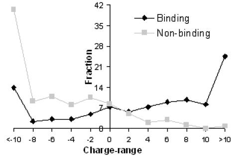
Distribution of overall charge for binding and non-binding cases in Electronic charge units (e). Labels on the x-axis indicate the upper value of the bin, e.g. 2 indicates the bin 0 to 2.

Thus, overall charge can be expected to distinguish the two cases with certain accuracy. Indeed, with this as the only feature combined with a linear classifier adopted from SVM, an accuracy value of 82.4% could be achieved with the jackknife evaluation method (Table 1).

Table 1.

Performance of the SVM for different combinations of descriptors, classifiers and evaluation techniques

Descriptor(s)	Classifier	Validation	Accuracy (%)	Sensitivity (%)	Specificity (%)	Parameters
						D	C	γ
Overall charge	Linear	Jackknife	82.4	58.6	95.7	1	11	0.01
Overall charge + patch size	Linear	Jackknife	83.8	60.3	96.6	1	13	0.02
All	Polynomial	Self-consistency	100	100	100	2	10	0.309
		Jackknife	90.5	81.8	94.9	2	19	0.054
		5-fold CV	89.1	82.1	93.9	2	19	0.051
		5-fold CV (20%)	90.3	67.4	94.9	2	23	0.034
All	Polynomial	Leave-half holdout	83.3	82.5	83.5	–	–	–
		Leave 1-pair holdout	86.3	80.6	87.5	–	–	–
		Leave 1-pair holdout (20%)	85.8	81.6	87.8	–	–	–

Reported in the last column are the parameters giving the corresponding accuracies. Sensitivity and specificity were defined as TP/(TP + FN) and TN/(TN + FP), respectively, where T = True, F = False, P = Positive and N = Negative.

Feature class 2: electrostatic patch

Since DNA is negatively charged, a large positive potential patch is deemed to be important in driving the protein to the DNA. The patches are calculated following the procedure described in Materials and Methods. Then the patches are sorted based on their sizes (number of atoms included in the patch) and the size of the largest patch is used as a descriptor.

To ascertain the propriety of this feature, we examined the overlap between our patches and the actual protein–DNA ‘interface’ atoms. A residue was designated as ‘interface’ residue if any heavy atom in that residue is closer than 4.5 Å to the DNA and the all its atoms were classified as ‘interface’ atoms. The overlap between interface and each positive patch was calculated and sorted (Figure 2). We found that in 63% of the DNA-BPs, the largest patch has the biggest overlap with the DNA-binding interface. For 20% of the proteins, the second largest patch has the largest overlap with the DNA interface. In only 1% (1 out of 120 proteins), the patch that had the largest overlay with the interface was not among the largest 5 in size. In 4% (5 cases), the DNA-binding interface has no overlap with positive patches.

Figure 2.

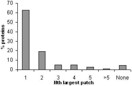
Overlap of the surface positive potential patches with the DNA-binding interface. x-axis represents the Nth biggest patch and y-axis exhibits the % of total binding proteins having the largest overlap with that patch. For example, 63% of the proteins had the largest overlap with the 1st largest patch.

When the above two features are combined for a linear classification of binding and non-binding proteins, we anticipate SVM to achieve a higher accuracy. Figure 3 plots the overall charge against the size of the largest patch for the binding (black) and the non-binding proteins (grey). In the intermediate range of the size of the largest patch, DNA-binding and non-DNA-BPs show some overlap but the separation becomes finer towards the higher extreme of the range. As expected, addition of size of the largest patch to overall charge as a feature vector further increases the accuracy values. With a linear classifier in SVM and these two features, DNA-BPs could be identified with 83.8% accuracy when evaluated on jackknife test.

Figure 3.

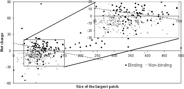
Linear separation of DNA-binding and non-DNA-BPs using only overall charge and size of the largest patch as the features as used by the SVM. Net charge is in electrostatic charge units.

Feature class 3: amino acid composition

Two kinds of amino acid composition are computed here: overall and surface (Figure 4). In case of overall composition, noticeable differences in binding and non-binding cases were observed with respect to the frequency of Lys and Arg. They both are positively charged amino acids so their over-representation in DNA-BPs is fairly implicit.

Figure 4.

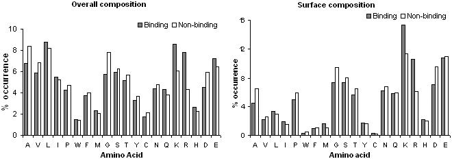
Frequency of different amino acids in overall and surface composition. The difference in the height of a bar for an amino acid for binding and non-binding cases reflects a stronger preference for that amino acid in one case over another.

As expected, surface composition was more disposed than overall composition for hydrophobic residues such as Trp, Phe, Tyr, Cys, Ile and Met. A higher frequency of Arg and Lys in binding proteins than non-binding ones was observed. A lower level of Asp can also be explained since DNA is negatively charge. Interestingly there is no difference between the frequencies of Glu. Other amino acids have the similar composition in both the binding and unbinding cases. From these observations one can expect that using composition alone won't be as efficient to linearly classify the DNA-BPs. So, we use them in conjunction with previously discussed features with non-linear kernel-based SVM.

Prediction of DNA-BPs

We combined all three classes of feature vectors and used them to train and test the SVM. For self-consistency, we could achieve an accuracy value of 100% (Table 1). This implies that SVM could cogently capture the intrinsic correlation between feature vectors and the classification being sought.

During CV, SVM is tested on how well it can predict on the basis of optimized parameters chosen during training. For both 5-fold CV and jackknife approaches employed, the performances of the current protocol were almost the same. Using Jackknife test, by optimizing the parameters with a polynomial kernel, we could achieve an accuracy value of 90.5% (325 correct predictions out of 359 cases) (Table 1). Corresponding sensitivity and specificity values were 81.8 and 94.9%. Similarly for a 5-fold CV technique, average correct predictions of 89.1% could be made with the optimum parameters with 82.1% sensitivity and 93.9% specificity (Table 1). Comparable values of sensitivity and specificity show that the performance of our protocol is poised.

To make sure that the performance of our protocol is not biased towards weak homology, we filtered the proteins using a sequence identity cut-off of 20% i.e. one of the proteins of all the pairs having >20% was removed. This assured that a protein in a test set has no sequence similarity at all to proteins in the train set. For the two sets we obtained accuracy values of 90.3%, which are very close to the accuracy value for the entire dataset (90.5%, Table 1). This shows that the above protocol was not biased due to homology recognition.

Finally, the holdout method is used for validation of the performance of current SVM protocol. The accuracy achieved in this test corresponds to the ones from true blind predictions. We iterated the method, which displayed a high deviation over 125 runs (Figure 5). Training accuracies varied from 79.8% to 92.7%, and testing accuracies ranged between 76.6% and 88.3%, with an average of 83.4%. Training accuracy was a little higher than testing accuracy because when SVM is being trained, it builds a classification model only on the basis of the training set, which is not optimized for the testing set. Overall the two accuracies showed a good correlation. To directly compare with the previous results (19), we also evaluated our performance for another holdout technique where a pair of DNA-binding and non-binding protein (selected randomly) was removed and the remaining dataset formed the training test. The left pair was then tested upon and this was repeated 500 times. Evaluated over these 1000 (500 × 2) predictions, we achieved an accuracy of 86.3%, (Table 1) which is higher than previously reported value of 83.9% (19).

Figure 5.

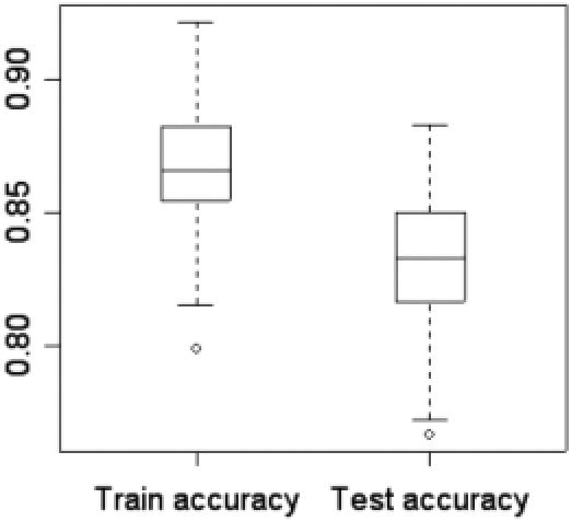
Box and whisker plot for the performance of the SVM for holdout technique. The performance data was collected over 125 runs.

Similar to the performance checking in CV, we also performed the leave-pair out hold out for reduced dataset that only proteins have <20% sequence identity are included. The accuracy value is 85.8%, which showed our protocol again doesn't depend on sequence homology to perform DNA-BP prediction. Online server has been provided with the current protocol on our webpage (http://proteomics.bioengr.uic.edu/pro-dna).

One class of non-DNA-BP is RNA-binding protein. Since RNA-binding protein do share similarities as DNA-BP (G. Zhao and H. Lu, unpublished data), it is expected our protocol may not perform as well when the negative cases are actually RNA-binding proteins. For this purpose, a list of 37 RNA-binding proteins was complied from ref. (36) and the features used above for classification were calculated. Using the model built from our previous dataset (none of the RNA-binding protein was included in optimization), the classification of RNA-binding protein resulted 21 correct prediction, and 16 wrong prediction. Thus we decided to perform a further binary classification model for the DNA- and RNA-binding proteins, this model resulted in 91.3% accuracy for the binary classification. Thus this post-processing can give reasonable accuracy to exclude RNA-binding proteins from the false positives in the DNA-BP predictions. It is an ongoing effort to design features specifically to distinguish the DNA-binding from RNA-binding proteins. The effort will naturally fall into the machine learning prediction categories.

We also attempted to identify DNA-BPs whose structure was solved without the DNA (the unbound cases). We found seven such proteins where native structures are available in both bound and unbound states. We structurally aligned the two states for each of the 7 cases using publicly available tool Superpose (37). RMSD values ranged from 0.53 Å to 5.11 Å between the corresponding structures. In SVM prediction, we used the built model where these 7 proteins were not included in the optimization process. Encouragingly, SVM classified correctly all of proteins using unbound structures. This shows that the above protocol can be used to identify DNA-BPs even before there is any deformation induced due to the binding of the DNA, if any.

Figure 6 shows three examples of different kinds of prediction results from SVM. In Figure 6A, 1 mjo was correctly classified as DNA-binding. The positive patches are near the DNA-binding surface. The structure of DNA was not used in the prediction and electrostatic calculation, nor was the information of binding sites. In this case, not only the protein is correctly classified, the positive patch can also give indications about the location of the binding site. Figure 6B shows another case where the protein (1 cma) was correctly predicted as DNA-binding one. Although, the largest patch is not so close to DNA, the 2nd and 3rd patches are very close to binding site. In this particular case, if we further want to push the idea of binding site prediction, other information in addition to location of patches would be added, as described in Bhardwaj and Lu (38). Finally there were about 10% of the cases where we incorrectly predicted the DNA binding behavior. Figure 6C is one of these cases (1 emh) that was misclassified as non-binding. In this protein, all the four positive patches are small and are far from the actual binding site (which we did not know during class prediction). Obviously this protein does not have features consistent with most of the other proteins and hence generic rules failed to classify it correctly. Such diverse behaviors show that more work needs to be done to add features to describe different DNA-binding mechanisms.

Figure 6.

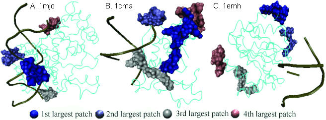
Orientation of the largest four patches with respect to the DNA. Remaining protein is shown in ‘tube’ representation in cyan. DNA is displayed in golden color with only backbone shown. Patches were mapped on the surface by adapting the PDB files for labeling the atoms in each patch and visualized in VMD (41).

DISCUSSION

We have implemented a kernel-based method (SVM) towards developing a robust protocol for identification of DNA-BPs. We have appraised the performance of the SVM using self-consistency, CV and holdout evaluation. We achieved an accuracy of 90% for CV and 100% for self-consistency. These values are higher than all previously published studies where the accuracy ranged from 67% to 86% (15–17,19). We also report accuracy value of 86.3% for leave 1-pair holdout technique, which is higher than that reported in a previous study using the same technique (19). Tsuchiya et al. (20), who used linear separation, reported 86% and 96% accuracy for DNA-binding and non-DNA-binding cases using self-consistency. Since SVM uses an entirely different strategy to achieve maximal self-consistency accuracy, there is no direct comparison between their values and self-consistency value of 100% reported in this paper.

Similar evaluation of CV and holdout have been applied to a more difficult (and smaller) test set where all proteins have less than 20% sequence identity. The accuracy achieved there, 90.3% for CV and 85.8% for holdout are comparable with the main results. These numbers demonstrate our protocol does not rely on even remote sequence homology for DNA-BP prediction.

We have used an ensemble of features describing DNA-BPs in order to distinguish them from non-DNA-BPs. Features used here show a varying distinction power. To judge the distinction power of a feature, we calculated Fisher's score (FS) for every feature, j as: $F{S}_j={({\mu }_1-{\mu }_2)}^2/s_1^2+s_2^2$ where μ_i and s_i are the mean and standard deviation of the feature in class i, respectively. Higher the FS, the more discriminative power this feature has. The top ten features with highest FS were: overall and surface fraction of Arg, overall charge, overall fraction of Gly, Asp, Lys, size of the largest patch, and the surface fraction of Asp, Lys and Gly. The greater discriminatory power of these features is also reflected in their contrasting distribution in the corresponding positive and negative cases. While it is expected the positive charged residues Arg, Lys and overall charge contribute to the good performance, there are some very interesting observations such as percentage of Gly plays important role in discriminating DNA-BPs. We have seen that there is less Gly in DNA-BP than in non-binding ones. This data may suggest that DNA-BPs in general are more rigid than non-binding ones.

Similarly, the top ten features showing highest power to distinguish DNA-BPs from RNA-binding ones were: overall fraction of His, largest patch size, overall charge, overall fraction of Trp, surface composition of Asp, Ile, His and Cys and overall fraction of Asp and Val. In this discrimination, we noticed besides the electrostatic properties, the percentage of His and Trp played important roles. Note, while Fisher's score indicates the predictive power of an individual feature, it is important to remember that the relationships between features that ultimately determine classification. Extracting and interpreting such information from an SVM model is still and open research issue.

As shown in the Results, these features when combined together can predict DNA-BPs from non-DNA-binding ones more accurately than when they are used separately. Apart from establishing the fact there is an inherent correlation between these features, this observation also authenticates the application of kernel-based machine learning methods to take advantage of this correlation.

The current implementation uses three classes of features and the results are highly encouraging. It is natural to assume with the inclusion of more features the performance will increase. A new class of features under development is the geometry of the protein surfaces. Encouragingly, it is easy to include new features in the framework of SVM. Further, when more features available, feature selection can be used to ascertain the features that are contributing more to the overall accuracy and the ones that are just adding noise.

Besides annexation of more features, a potential channel for furthering the prediction power of the SVM would be through development of models specific to a class, a family or even motifs (39). To begin with, trends specific to some structural motifs that play a key role in binding to the DNA, such as helix–turn–helix or helix–loop–helix, could be included (40). Also, deciphering the reasons why some particular sites on the surface bind to the DNA and others do not will go a long way in improving our understanding of the determinants of DNA-binding. For misclassified proteins, it would be tempting to uncover the driving forces and agents behind both mobilization of such erratic proteins to the DNA and, selection of the binding sites.

The development of the above protocol is purported to augment contemporary function annotation tools. Since this protocol does not rely on any sequential or structural analogy, it is capable of identifying DNA-BPs even when they are embedded in novel motifs or folds. In the future course of exploration in related fields we contemplate a multitude of kernel-based machine-learning tools to be employed for the purpose of DNA-BPs identification. The method can apparently be polished by addition of more features and apt fine-tuning of the SVM once the circumstances of protein–DNA-binding are better comprehended.

REFERENCES

- 1.Luscombel N.M., Austin S.E., Berman H.M., Thornton J.M. An overview of the structures of protein–DNA complexes. Genome Biol. 2000;1:1–37. doi: 10.1186/gb-2000-1-1-reviews001. [DOI] [PMC free article] [PubMed] [Google Scholar]
- 2.Jones S., Heyningen P., Berman H.M., Thornton J.M. Protein–DNA interactions: a structural analysis. J. Mol. Biol. 1999;287:877–896. doi: 10.1006/jmbi.1999.2659. [DOI] [PubMed] [Google Scholar]
- 3.Siggers T.W., Silkov A., Honig B. Structural alignment of protein–DNA interfaces: insights into the determinants of binding specificity. J. Mol. Biol. 2005;345:1027–1045. doi: 10.1016/j.jmb.2004.11.010. [DOI] [PubMed] [Google Scholar]
- 4.Pabo C.O., Nekludova L. Geometric analysis and comparison of protein–DNA interfaces: why is there no simple code for recognition? J. Mol. Biol. 2000;301:597–624. doi: 10.1006/jmbi.2000.3918. [DOI] [PubMed] [Google Scholar]
- 5.Nadassy K, Wodak S.J., Janin J. Structural features of protein-nucleic acid recognition sites. Biochemistry. 1999;38:1999–2017. doi: 10.1021/bi982362d. [DOI] [PubMed] [Google Scholar]
- 6.Alexander M.K., Bourns B.D., Zakian V.A. One-hybrid systems for detecting protein–DNA interactions. Methods Mol. Biol. 2001;177:241–259. doi: 10.1385/1-59259-210-4:241. [DOI] [PubMed] [Google Scholar]
- 7.Sathyapriya R., Vishveshwara S. Interaction of DNA with clusters of amino acids in proteins. Nucleic Acids Res. 2004;32:4109–4118. doi: 10.1093/nar/gkh733. [DOI] [PMC free article] [PubMed] [Google Scholar]
- 8.Havranek J.J., Duarte C.M., Baker D.J. A simple physical model for the prediction and design of protein–DNA interactions. J. Mol Biol. 2004;344:59–70. doi: 10.1016/j.jmb.2004.09.029. [DOI] [PubMed] [Google Scholar]
- 9.Benos P.V., Lapedes A.S., Stormo G.D. Is there a code for protein–DNA recognition? Probab(ilistical)ly. Bioessays. 2002;24:466–475. doi: 10.1002/bies.10073. [DOI] [PubMed] [Google Scholar]
- 10.Paillard G., Lavery R. Analyzing protein–DNA recognition mechanisms. Structure. 2004;12:113–22. doi: 10.1016/j.str.2003.11.022. [DOI] [PubMed] [Google Scholar]
- 11.Djordjevic M., Sengupta A.M., Shraiman B.I. A biophysical approach to transcription factor binding site discovery. Genome Res. 2003;13:2381–2390. doi: 10.1101/gr.1271603. [DOI] [PMC free article] [PubMed] [Google Scholar]
- 12.Marcotte E.M., Pellegrini M., Ng H.-L., Rice D.W., Yeates T.O., Eisenberg D. Detecting protein function and protein–protein interactions from genome sequences. Science. 1999;285:751–753. doi: 10.1126/science.285.5428.751. [DOI] [PubMed] [Google Scholar]
- 13.Lu X., Zhai C., Gopalakrishnan V., Buchanan B.G. Automatic annotation of protein motif function with Gene Ontology terms. BMC Bioinformatics. 2004;5:122. doi: 10.1186/1471-2105-5-122. [DOI] [PMC free article] [PubMed] [Google Scholar]
- 14.Pellegrini M., Marcotte E.M., Thompson M.J., Eisenberg D., Yeates T.O. Assigning protein functions by comparative genome analysis: protein phylogenetic profiles. Proc. Natl Acad. Sci. USA. 1999;96:4285–4288. doi: 10.1073/pnas.96.8.4285. [DOI] [PMC free article] [PubMed] [Google Scholar]
- 15.Cai Y., Lin S.L. Support vector machines for predicting rRNA-, RNA-, and DNA-binding proteins from amino acid sequences. Biochim. Biophys. Acta. 2003;1648:127–133. doi: 10.1016/s1570-9639(03)00112-2. [DOI] [PubMed] [Google Scholar]
- 16.Ahmad S., Gromiha M.M., Sarai A. Analysis of DNA-binding proteins and their binding residues based on composition, sequence and structural information. Bioinformatics. 2004;20:477–486. doi: 10.1093/bioinformatics/btg432. [DOI] [PubMed] [Google Scholar]
- 17.Stawiski E.W., Gregoret L.M., Mandel-Gutfreund Y. Annotating nucleic acid-binding function based on protein structure. J. Mol. Bio. 2003;326:1065–1079. doi: 10.1016/s0022-2836(03)00031-7. [DOI] [PubMed] [Google Scholar]
- 18.Jones S., Shanahan H.P., Berman H.M., Thornton J.M. Using electrostatic potentials to predict DNA-binding sites on DNA-binding proteins. Nucleic Acids Res. 2003;31:7189–7198. doi: 10.1093/nar/gkg922. [DOI] [PMC free article] [PubMed] [Google Scholar]
- 19.Ahmad S., Sarai A. Moment-based prediction of DNA-binding proteins. J. Mol. Biol. 2004;341:65–71. doi: 10.1016/j.jmb.2004.05.058. [DOI] [PubMed] [Google Scholar]
- 20.Tsuchiya Y., Kinoshita K., Nakamura H. Structure-based prediction of DNA-binding sites on proteins using empirical preference of electrostatic potential and the shape of molecular surfaces. Proteins. 2004;55:885–894. doi: 10.1002/prot.20111. [DOI] [PubMed] [Google Scholar]
- 21.Vapnik V., Cortes C. Support vector networks. Machine Learning. 1995;20:273–293. [Google Scholar]
- 22.Dubchak I., Muchnik I., Mayor C., Dralyuk I., Kim S.-H. Recognition of a protein fold in the context of the Structural Classification of Proteins (SCOP) classification. Proteins. 1999;35:401–407. [PubMed] [Google Scholar]
- 23.Brown M.P., Grundy W.N., Lin D., Cristianini N., Sugnet C.W., Furey T.S., Ares M., Jr, Haussler D. Knowledge-based analysis of microarray gene expression data by using support vector machines. Proc. Natl Acad. Sci. USA. 2000;97:262–267. doi: 10.1073/pnas.97.1.262. [DOI] [PMC free article] [PubMed] [Google Scholar]
- 24.Jaakkola T., Diekhans M., Haussler D. Proc. Seventh Int. Conf. Intell. Syst. Mol. Biol. Menlo Park, CA: AAAI Press; 1999. Using the Fisher kernel method to detect remote protein homologies; pp. 149–158. [PubMed] [Google Scholar]
- 25.Ding C.H.Q., Dubchak I. Multi-class protein fold recognition using support vector machines and neural networks. Bioinformatics. 2001;17:349–358. doi: 10.1093/bioinformatics/17.4.349. [DOI] [PubMed] [Google Scholar]
- 26.Langlois R.E., Diec A., Perisic O., Dai Y., Lu H. Improved Protein Fold Assignment Using Support Vector Machines. Int J Bioinformatics Research and Applications. 2005 doi: 10.1504/IJBRA.2005.007909. (In Press) [DOI] [PubMed] [Google Scholar]
- 27.Jones S., Shanahan H.P., Berman H.M., Thornton J.M. Using electrostatic potentials to predict DNA-binding site on DNA-binding proteins. Nucleic Acids. Res. 2003;31:7189–7198. doi: 10.1093/nar/gkg922. [DOI] [PMC free article] [PubMed] [Google Scholar]
- 28.Word J.M., Lovell S.C., Richardson J.S., Richardson D.C. Asparagine and glutamine: using hydrogen atom contacts in the choice of side-chain amide orientation. J. Mol. Biol. 1999;285:1735–1747. doi: 10.1006/jmbi.1998.2401. [DOI] [PubMed] [Google Scholar]
- 29.Brooks B., Bruccoleri R.E., Olafson B., States D., Swaminathan S., Karplus M. CHARMM: a program for macromolecular energy, minimization, and dynamics calculations. J. Comput. Chem. 1983;4:187–217. [Google Scholar]
- 30.Gilson M., Sharp K., Honig B. Calculating electrostatic interactions in bio-molecules: method and error assessment. J. Comput. Chem. 1988;9:327–335. [Google Scholar]
- 31.Jayaram B., Sharp K.A., Honig B. The electrostatic potential of B-DNA. Biopolymers. 1989;28:975–993. doi: 10.1002/bip.360280506. [DOI] [PubMed] [Google Scholar]
- 32.Sharp K.A., Honig B. Electrostatic interactions in macromolecules: theory and applications. Annu. Rev. Biophys. Biophys. Chem. 1990;19:301–332. doi: 10.1146/annurev.bb.19.060190.001505. [DOI] [PubMed] [Google Scholar]
- 33.Kabsch W., Sander C. Dictionary of protein secondary structure: pattern recognition of hydrogen-bonded and geometrical features. Biopolymers. 1983;22:2577–2637. doi: 10.1002/bip.360221211. [DOI] [PubMed] [Google Scholar]
- 34.Cristianini N., Shawe-Taylor J. Cambridge, UK: Cambridge University Press; 1999. An Introduction to Support Vector Machines and Other Kernel-Based Learning Methods. [Google Scholar]
- 35.Chang C.-C., Lin C.-J. LIBSVM: A Library for Support Vector Machines. 2005. Technical Report. Department of Computer Science, National Taiwan University.
- 36.Chen Y., Kortemme T., Robertson T., Baker D., Varani G. ‘A new hydrogen-bonding potential for the design of protein–RNA interactions predicts specific contacts and discriminates decoys’. Nucleic. Acids Res. 2004;32:5145–6162. doi: 10.1093/nar/gkh785. [DOI] [PMC free article] [PubMed] [Google Scholar]
- 37.Maiti R., Van Domselaar G.H., Zhang H., Wishart D.S. SuperPose: a simple server for sophisticated structural superposition. Nucleic Acids Res. 2004;32:W590–594. doi: 10.1093/nar/gkh477. [DOI] [PMC free article] [PubMed] [Google Scholar]
- 38.Bhardwaj N., Langlois R.E., Zhao G., Lu H. Structure Based Prediction of Binding Residues on DNA-binding Proteins. 27th Annual International Conference of the Engineering in Medicine and Biology Society; 2005. (in press) [DOI] [PubMed] [Google Scholar]
- 39.Harrison S.C. A structural taxonomy of DNA-binding domains. Nature. 1991;353:715–719. doi: 10.1038/353715a0. [DOI] [PubMed] [Google Scholar]
- 40.Jones S., Barker J.A., Nobeli I., Thornton J.M. Using structural motif templates to identify proteins with DNA binding function. Nucleic Acids Res. 2003;31:2811–2823. doi: 10.1093/nar/gkg386. [DOI] [PMC free article] [PubMed] [Google Scholar]
- 41.Humphrey W., Dalke A., Schulten K. VMD: visual molecular dynamics. J. Mol. Graph. 1996;14:33–38. doi: 10.1016/0263-7855(96)00018-5. [DOI] [PubMed] [Google Scholar]