Turbulence in nature and in the laboratory

Abstract

Fluid turbulence has attracted the attention of physicists, mathematicians, and engineers for over 100 years, yet it remains an unsolved problem. The reasons for the difficulties are outlined and recent advances in describing its small-scale statistical structure are described. Contrary to traditional notions, new experimental evidence indicates that the small scales are anisotropic, reflecting the overall character of the flow. The consequences of this finding with regard to the long-held postulate of the universality of the small-scale turbulence structure are discussed.

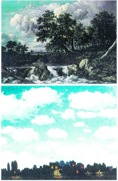
The great cloud paintings of Ruisdael and Magritte (Fig. 1) beautifully express the way we characterize turbulence in modern texts: it is irregular, has strong vorticity, causes rapid mixing (a blob of dye would rapidly disperse in Ruisdael's turbulent waters), and is a multiscale phemonenon. Fig. 2, a mural in a Greek restaurant near Fort Myers, FL, is unconvincing because it misses the vital multiscale characteristic. All eddies are the same size. If this were in fact the case, there would be no turbulence problem. The essence of turbulence is its multiscale behavior.

Fig 1.

(Upper) Waterfall by Jacob Van Ruisdael (1628–1682). Rijks Museum, Amsterdam. (Lower) The Empire of Lights by René Magritte (1898–1967). [Reproduced with permission (Copyright 2001, Charly Herscovici, Brussels/Artists Rights Society, New York).]

Fig 2.

Mural in a Greek restaurant, Fort Myers, FL. Photo by author.

Because the largest length scales (ℓ) are typically of the order of 1 km in a cumulous cloud, and the fluctuating turbulent velocities (u) are of the order of meters per second, the clouds in the pictures are extremely turbulent, indicating a highly mixed state. This is characterized by the Reynolds number

which is the ratio of the inertial forces (which describe the fluid acceleration) to viscous forces (which inhibit the fluid motion). It is very high; of the order 10⁸. (Here ν is the kinematic viscosity of order 10⁻⁵ m²⋅s⁻¹ in a cloud.) Yet what is striking is the complexity of the structures. No two clouds are alike. We wonder whether any universal characteristics are present. Can the scientist generate high Reynolds number turbulence in the laboratory in such a way that it reduces the complexity, yet retains the essential ingredients of the high Reynolds number turbulence?

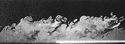
When we set up an ideal turbulent flow in the laboratory, we obtain images like that shown in Fig. 3 (1). This is a boundary layer. A carefully controlled wind of constant mean velocity is driven (by a fan) over a perfectly flat plate. The “no slip” condition (e.g., ref. 2) forces the air motion to be zero at the plate itself, thereby inducing a velocity gradient or shear in the flow. Unlike the situations of Fig. 1, here the boundary conditions are carefully controlled. Yet the resulting picture appears to be just as complex. Apparently, simplifying the boundary conditions does not help us very much. It is difficult to reduce the complexity of the turbulence much more than this, although slightly simpler flows can be contrived.

Fig 3.

A turbulent boundary on a wall. [Reproduced with permission from ref. 1 (Copyright 1977, American Institute of Physics).]

There are thousands of papers on turbulent boundary layers, and the subject is still a fertile research area. Boundary layers occur on the surface of airplane wings, turbine blades, and the Earth. They affect the drag properties, as well as the dispersion of pollution and the formation of clouds (which in the Magritte picture are sitting atop the planetary boundary layer). Pipe flows, jets, wakes, and convection in a box are other standard laboratory flows. They are equally complex and the “solution” of one will have direct ramifications for them all. Yet we still do not have anywhere near a solution to any of these problems in the sense, say, that we have a solution to the hydrogen atom or to critical point phenomena. Feynman (3), writing in the 1960s is still up to date: “Finally, there is a physical problem that is common to many fields, that is very old, and that has not been solved … It is the analysis of circulating or turbulent fluids … The simplest form of the problem is to take a pipe that is very long and push water through it at high speed. We ask: to push a given amount of water through that pipe, how much pressure is needed? No one can analyze it from first principles and the properties of water. If the water flows very slowly, or if we use a thick goo like honey, then we can do it nicely. You will find that in your textbook. What we really cannot do is deal with actual, wet water running through a pipe. That is the central problem which we ought to solve some day, and we have not.”

The Turbulence Problem

It is difficult to think of a physics problem that can apparently be so clearly stated that has evaded a solution for so long.

Why is the turbulence problem so difficult? The equation of fluid motion, the Navier Stokes equation

is a nonlinear partial differential equation. As Feynman states, there are solutions to this equation for simple laminar flows, like honey flowing down a plate, that occur at low Reynolds numbers. But at high Reynolds numbers the essence of the problem lies in the nonlinearity. It is not possible to develop a perturbation theory around the linear part of the equation because the theory has no small parameter: quadratic and higher-order terms are the essential ingredients of the problem. Thus perturbation expansions are strongly divergent. In this regard the Navier Stokes equations are the most intractable of all of the field equations we know, including those of general relativity. Osborn Reynolds (4) realized the heart of the problem in the late nineteenth century. He decomposed the velocity component V into a mean (U) and a fluctuation (u), i.e., V = U + u. Thus for a waterfall U is its average speed and u are fluctuations of the flow about this average; the jittering motion that a speck of dust would undergo while being advected along by the water. [Even earlier Leonardo da Vinci, hinting at this decomposition (5), likened turbulent flow to the way hair falls (the mean motion), and curls (the fluctuations), on the nape of a woman's neck]. Substituting U + u for V in Eq. 2 generates high-order terms for the fluctuating components. These terms are generally of the same order as the lower-order ones. Engineers, who seek solutions for real flows, attempt to “close” the equations by modeling the higher-order terms in terms of the lower orders. The success in this direction has been significant (e.g., refs. 6–8) but such an approach does not satisfy the mathematician or physicist. Because a field theoretical solution of the Navier Stokes equation is elusive (e.g., ref. 9), the fruitful approach comes from asking questions concerning the physics of the processes. Here I turn away from the equations of motion and construct physical models. I ask: Are there any universal aspects of turbulent flow? Figs. 1 and 3 suggest that the largest scales depend on the way the turbulent flow is formed, and therefore are definitely non-universal. They provide the flow with its special character, be it a cloud, smokestack jet, or waterfall. But what about the smaller scales? If one takes a cubic meter inside a cloud, say, and a cubic meter of a volcanic plume, or of a smoke stack, is it possible that of these scales the turbulence may look the same? (Of course the picture may have to be scaled by magnifying one relative to another.) Our present view of turbulence suggests this is the case, at least to a good first approximation.

Our “standard model” comes from Kolmogorov (10) who in 1941 postulated that there is a cascade of turbulence energy from largest eddies to smallest eddies (or scales). The rate of energy input (per unit mass) at the largest scales is equal to the energy through-put from the large to the small scales. This rate, in turn, is equal to the energy dissipated by the smallest scales. If we rapidly stir the bath with a large arm action and then withdraw our hand, the energy is passed this way to the small scales. The motion ceases, and the bath is slightly warmer. Turbulence is highly dissipative. Notice how rapidly the turbulence ceases (in contrast to the residual wave motion).

Because the average rate of energy dissipation (per unit mass), 〈ɛ〉 m²/s³, is the same as the average rate of energy input, it is determined from the large-scale quantities: the average kinetic energy per unit mass of the large eddies, u², and their characteristic “turn over time” (the lifetime of the eddy), ℓ/u. Thus

where, both u and ℓ (as in Eq. 1) are average statistical quantities (root mean square quantities). The model, Eq. 3, works extremely well, and must be regarded as basic a law that we have in turbulence. It allows us to model 〈ɛ〉, a vital step in closing the turbulence equations. It also allows us to determine the power of a cloud, or other turbulent flows, from simple estimates of their size and characteristic turbulence velocities. For example, for a typical cumulus cloud, ℓ ∼1 km and u ∼1 m/s. Hence 〈ɛ〉∼10⁻³ m²/s³ and the total power (〈ɛ〉ρℓ³ where ρ is the density, taken here as 1 kg/m³) is 1 megawatt. Volcanic plumes and the Earth's boundary layer dissipate even greater amounts of energy.

According to Kolmogorov, as the cascade proceeds the successive generations of smaller eddies lose information of the large-scale structure of the flow. Thus the anisotropy of the large scales fades and the small scales become statistically isotropic. Our snapshot of the cubic meter of cloud could be rotated and reflected without our being concerned. On the other hand, a slight rotation of the large scales (a complete cloud, Fig. 1) will tell us something is wrong. That a cascade picture seems reasonable was appreciated earlier on by L. F. Richardson (10). The fact that large-scale forcing produces a myriad of smaller scales is evident to anyone who has stirred a bath. What was new from Kolmogorov (published in 1941 and known as K41), is the notion of local isotropy, the isotropy of the small scales. Further, Kolmogorov postulated that the statistics of these isotropic scales would have universal behavior, independent of the way the flow was produced, be it in a cloud, a jet, or a waterfall. The scales at which this approximately occurs are known as the universal equilibrium subrange. This is further divided into a dissipation subrange (the very smallest scales) and the inertial subrange, those scales larger than the dissipation scales (where viscosity becomes dominant), but smaller than the large anisotropic scales that define the flow. In the Magritte clouds (Fig. 1b) the inertial subrange may be of the order meters to millimeters. Its width increases as the Reynolds number increases (more vigorous stirring, or an increase of the scale of the flow); as the Reynolds number increases the anisotropic large scales encroach less and less on the smallest scales.

In the inertial subrange K41 provides predictions for the way the statistics of velocity differences, across a separation, r, behave. Defining this difference u(R + r) − u(R), (where R is a reference point) as Δu(r), K41 predicts that its statistical average (ensemble or time average) will be only a function of 〈ɛ〉 and r itself. Thus, the structure function, 〈(Δu(r))ⁿ〉, scales as

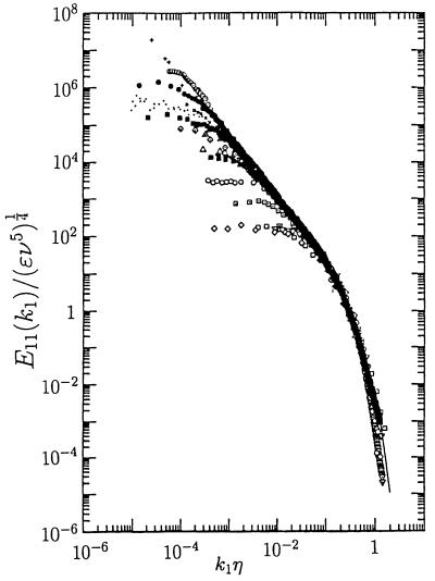
For n = 2, the variance 〈(Δu(r))²〉 will increase as r^2/3. For this case the Fourier transform of Eq. 4 yields a −5/3 spectrum (11). It has been verified in many flows (Fig. 4).

Fig 4.

The turbulence spectrum measured in many different flows. As the Reynolds number increases, the width of the spectrum increases, as the large scales are separated further from the small scales. At high Reynolds number, Kolmogorov (10) predicts a slope of −5/3, which is seen in these measurements. [Reproduced with permission from ref. 11 (Copyright 1994, Cambridge University Press).]

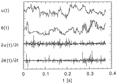
K41 is a pillar of modern turbulence theory. Its prediction for second-order quantities is remarkable, and its effect on modeling real turbulent flows cannot be underestimated. Yet soon after it appeared some insurmountable problems became apparent. The dissipation rate was found to vary both spatially and temporally within the flow. Because the ultimate fate of the turbulence energy is at the small scales, the dissipation rate is related to the sharp gradients of the velocity that occur there. Thus the dissipation is a function of various combinations of the velocity derivatives. Fig. 5 shows a time series of one velocity derivative, ∂u/∂t, in a turbulent flow. The velocity fluctuations themselves (the u trace) are close to Gaussian, but those of ∂u/∂t are strongly non-Gaussian. This finding implies that dissipation in turbulent flows is “spotty” or intermittent. There are moments when it is large, followed by quieter moments. In Kolmogorov the governing parameter is the average dissipation rate.

Fig 5.

Time series of the longitudinal velocity fluctuations, u(t), and their derivative, ∂u(t)/∂t. Also shown is the time series of scalar fluctuations, θ(t), and their derivative, ∂θ(t)/∂t, in the same flow. Notice the higher intermittency in the scalar (bottom trace). R_λ = 582. Measurements by L. Mydlarski and Z.W.

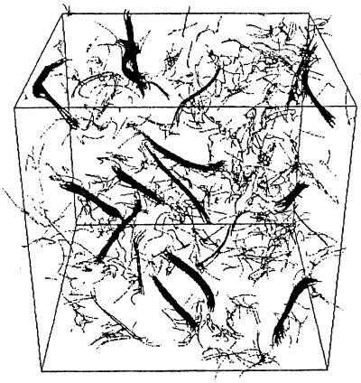
Intermittency (Fig. 5) was first observed by Batchelor and Townsend in 1949 (12), but was anticipated independently by Landau [see Frisch (10)]. He argued that small fluctuations of ɛ will be successively amplified as the cascade proceeds. The turbulence becomes “lumpy,” and complex structures are implied. These were later observed in experimental as well as computer simulations (Fig. 6; ref. 13). Although the individual structures are clearly anisotropic, there is a possibility that their statistical variation is such that the turbulence remains isotropic, so that the notion of universality may still not be lost. However, it will be shown that this does not appear to be the case.

Fig 6.

Numerical simulation of vortex filaments in a turbulent fluid. [Reproduced with permission from ref. 13 (Copyright 1991, The Royal Society of London).]

The intermittent nature of the velocity dissipation, which is evident both at the dissipation and inertial scales, suggests that the turbulence may not be a self similar process: enlargement of a section of the time series of Fig. 5a will not produce a time series that is statistically similar to the original one. The qualitative nature of the time series changes as one looks successively at more detailed enlargements. This aspect presents immense difficulties for the theoretician.

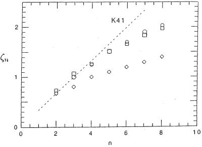
If structure functions from the time series of Fig. 5a are constructed, a linear trend in the scaling exponent [as predicted by K41 (Eq. 4)] is not found; it is nonlinear, with increasing departure from K41 with increasing n. A plot of the scaling exponent is shown in Fig. 7. Notice that at second order K41 still holds extremely well. The departure from linearity at higher orders is caused by the intermittent nature of the turbulence.

Fig 7.

Inertial subrange scaling exponents for velocity and scalar structure function, ζ_n. Longitudinal velocity component measured along the mean velocity gradient (○) and transverse to it (□). The scalar structure function exponent (◊). Both the velocity and scalar depart from the K41 prediction (Eq. 4) for higher orders, with the scalar showing a greater departure. This is consistent with its greater intermittency, Fig. 5. [Reproduced with permission from ref. 15 (Copyright 2000, Annual Reviews).]

It is apparent that the two quantities 〈ɛ〉 and r are not enough to determine the form of the structure function. A new parameter must enter. Usually the integral length scale is introduced (10), and we write

where ζ_n = n/3 − δ_n is the scaling exponent and δ_n is the departure from K41. [For δ_n = 0 (4) reduces to K41, Eq. 4.] The issue is to determine ζ_n.

Virtually all theories are based on the cascade model. Simple fractal models (10) provided starting points for later developments. Here at each stage of the cascade the number of “daughters” of a given “mother” eddy is chosen such that the fraction of volume occupied is decreased by a factor β(0 < β < 1). This scheme, known as the β model, allows for the intermittency to occur. There is one adjustable parameter, D, the fractal dimension, and for D = 3, K41 is retrieved. Although insightful, the model incorrectly predicts a linear dependence of ζ_n on n. More advanced models (10) describe the inertial subrange cascade as a random multiplicative process and use a multifractal approach. Some of these models produce scaling exponents that are close to the data of Fig. 7. Yet there is something unsatisfying, in a similar way that attempts to fit curves through the black body radiation curve were unsatisfying before Planck's momentous insight.

Is the Postulate of Local Isotropy Correct?

The cascade concept and the postulate of local isotropy are tightly bound. If local isotropy did not hold, the implication would be that the small scales are not universal and that there is direct interaction between the large and the small scales.

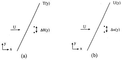
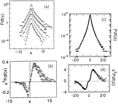
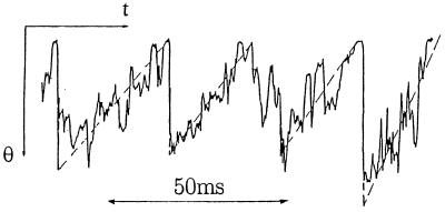
It has been known for over 30 years (14–16) that fluctuating passive scalars, such as low concentrations of dye in water, or humidity or temperature in air, are anisotropic at the small scales. If, for example, a large-scale mean scalar gradient is imposed on a turbulent velocity field, say by gently heating one side of the flow (Fig. 8a), the resultant small-scale temperature fluctuations reflect the large-scale gradient. This is manifest in the probability density function (pdf) of the scalar derivative (measured along the gradient) having asymmetric tails. The pdf is skewed (Fig. 9a). If the sign of the gradient is flipped, the sign of the skewness is reversed (the tail would be broader on the left side rather than the right side of Fig. 9a). An examination of the time series of the temperature fluctuations along the mean gradient shows ramp-cliff structures (Fig. 10).

Fig 8.

A simple way to impose large-scale anisotropy on a flow is to impose a linear variation of the mean quantity. (a) A mean scalar gradient [temperature, T(y)] is applied to an isotropic turbulent field. (b) The velocity field is sheared, providing the variation in its mean, U(y). To investigate the small-scale structure, difference, and derivative measurements are made along the gradient [Δθ(y) and Δu(y) for the scalar (temperature) and velocity, respectively]. If local isotropy were to hold, then the odd moments should be zero for small displacements.

Fig 9.

pdfs of the scalar (a) and velocity (c) derivatives measured along their respective mean gradients. The pdfs are not symmetrical: asymmetry is observed at the third moment for the scalar (b), and at the fifth moment for the velocity (d). The anisotropy appears to be independent of Reynolds number (17, 21). In a and b, x ≡ ∂θ/∂y/〈(∂θ/∂y)²〉^1/2, and in c and d, z ≡ ∂u/∂y/〈(∂u/∂y)²〉^1/2. [a and b, Reproduced with permission from ref. 17 (Copyright 1994, American Institute of Physics).] [c and d, Reproduced with permission from ref. 21 (Copyright 2000, American Institute of Physics).]

Fig 10.

Time series of a passive scalar (temperature) from a heated jet showing ramp-cliff structures. [Reproduced with permission from ref. 18 (Copyright 1979, Cambridge University Press).]

Insightful numerical simulations of Holzer and Siggia (19) have shown that along with the anisotropy comes intermittency. They generate a strictly Gaussian velocity field, i.e., one with no internal intermittency or structure at all, and impose on this a passive scalar gradient. They find skewed pdfs similar to those of Fig. 9a, and an intermittent time series for the derivative of the temperature fluctuations, similar to that of Fig. 5 (bottom trace). The turbulent mixing by the large eddies expels the large-scale gradient and forms patches of approximately constant scalar concentration. They observe cliffs and show they are sharp fronts produced by the large-scale overturning of the velocity field: the interface of a large downward (warm) eddy and an upward (cool) eddy. The width of those fronts is small, and so large and small scales are directly coupled. The fronts not only cause the pdf to be skewed, but they affect the higher moments, causing non-Gaussian even ones that we associate with intermittency. The fact that a purely Gaussian field could produce scalar intermittency was realized early by Kraichnan (20). What is new here is that the intermittency and anisotropy are intimately connected.

What about the velocity field itself? Here, too, we can impose large-scale anisotropy on the flow by forming a shear. In a wind tunnel we can contrive a flow with constant shear (shown schematically in Fig. 8b) by means of a series of screens set up to differentially block the flow. When one does this type of experiment a similar effect to that observed for the scalar is found, but it is more subtle. The pdf of the velocity is also skewed, but the skewness is manifest in the fifth rather than the third moment (21) (Fig. 9d). Thus for the velocity field, the events (sharp fronts) reaching the small scales directly from the large scales are more rare and more intense. The weaker ones do not penetrate.

The results concerning the anisotropy of the velocity field are new and require careful evaluation by other laboratories. One prerequisite is that the Reynolds number must be very high so that there is enough separation between the large and small scales, otherwise we would expect the large scales to directly affect the small ones. How high must the Reynolds number be? Again we do not know the answer to this question. The Reynolds number (defined in Eq. 1) of the experiments in ref. 21 was close to 10⁵. The highest Reynolds numbers are in the atmosphere and oceans, where they can be 2 or 3 orders of magnitude greater. However, checking this delicate measurement in geophysical flows is difficult because of statistically nonstationary effects.

The new results show that the large-scale organization of the flow is reflected at the small scale. They provide a way of understanding intermittency that is different to the cascade notion. What if the shear is turned off and the large scales are isotropic? Clearly the small scales should be isotropic for this condition, and this is observed in laboratory flows. But here, too, there will be clashes of large eddies, and at their interface there will be sharp jumps in the velocity. The large eddies will be randomly oriented (in the shear flow they are aligned by the shear) and so there will be no preferred direction, and no asymmetry in the pdf, but still there will be intermittency. Here, too, then, intermittency will be the result of the direct interaction of large and small scales. Here, too, extremely intense and rare events will be directly communicated to the small scales.

The above discussion of the pdfs (Fig. 9) pertains to the very smallest scales—the dissipation range. There is also very good evidence for the connection between intermittency and anisotropy in the inertial subrange. If we determine a structure function in shear flow by moving one velocity probe in the shear direction relative to another fixed one, we can determine the transverse structure function of u (Fig. 8b). The odd order transverse functions exist solely because of the anisotropy of the flow. Remarkably, the experiments show that their magnitude is of the same order as the even ones, and their scaling exponents are such that they increase (with increasing order) in a similar way to the even ones (21). This implies that the anomalous scaling (i.e., the departure from K41) can be accounted for solely in terms of the anisotropy, because the odd moments (which isotropy requires to be zero) capture the full anomaly. The transverse scaling exponents are also shown on Fig. 7.

These recent results not only suggest that the postulate of local isotropy is incorrect, but they also give a strong indication that intermittency and anisotropy result from the same cause: rare intense events at the integral scale that directly couple to the small scales. Although the early experimental evidence is compelling, much work will be required to base a sound theory on those observations.

The State of the Subject

It may seem remarkable that such a basic question as to whether the small scales are isotropic or not has not been definitively answered. After all, the subject is over 100 years old and the only medium required for its study is air or water. Part of the problem is analogous to that encountered by high-energy physicists. To understand the ultimate structure of matter higher and higher energies are needed, and hence the need for expensive accelerators. In turbulence, higher and higher Reynolds numbers are needed to separate the large scales from the inertial ones, where some kind of order may be found. One of the advances in the past decade has been in the development of new devices to produce controlled high Reynolds number turbulence in the laboratory (21–24). Nevertheless the Reynolds numbers achieved so far still fall short of those required.

But turbulence is not only a basic scientific problem but also one of great practical importance. So I return to the large scales and engineering considerations. I have mentioned that it is the largest scales that provide the flow with its particular character; they determine rate at which a smoke plume spreads, the stress on the surface of a pipe, and the depth of the atmospheric boundary layer. How do we calculate these characteristics? One obvious approach is to solve the Navier Stokes equation by direct numerical simulation. This approach requires very large computers: the ratio of the largest (ℓ) to the smallest (η) scales varies as ℓ/η∼(Re)^3/4. [Because the smallest scale in the cascade, η, can only be a function of 〈ɛ〉 and ν (the former driving the cascade to the smaller scales, the latter inhibiting the cascade at the smallest scales) dimensional analysis yields η∼(ν³/〈ɛ〉)^1/4. Using this as well as Eqs. 1 and 3 the result ℓ/η∼(Re)^3/4 is obtained.] For a cloud, Re∼10⁸, so ℓ/η∼10⁶. The number of grid points required to completely compute the flow in three dimensions is the cube of this, 10¹⁸ grid points. To follow the evolution of all of the details of a cloud for one characteristic eddy evolution time (ℓ/u∼10 min for a typical cumulous cloud) would take many thousands of years in today's largest computers (25). For this reason direct numerical simulation is confined to flows of relatively small Reynolds numbers, and with relatively simple geometry (flow in a duct rather than flow over a rotating turbine blade, for example).

The fact that there appears to be some level of universality, at least to second order (Fig. 4), suggests that the small scales could be parameterized, leaving only the large scales to be directly computed. This approach, known as large eddy simulation (LES), is considered by many to be extremely promising (26) because in direct numerical simulation most of the time is spent computing the small scales. In LES, by foregoing the small scales, relatively high Reynolds numbers can be obtained, and many of the real characteristics of the turbulence can be captured. It has been successfully applied to homogeneous turbulence, jets, wakes, and transitional flows (26). Although still in its infancy, the level of research activity suggests it may become a major tool, possibly replacing single point closures (6–8) (which only provide information on averaged quantities such as variances and stresses) as the major work horse.

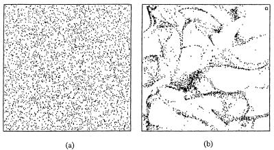
Yet in this brief review I have stressed that the behavior of the small scales may be directly determined by the large scales. Although this may not matter for some practical applications (because it pertains mainly to the higher-order moments) it would seem that to understand such major problems as mixing, reactions, and combustion, as well as nucleation in clouds, both the small and large scales will have to be studied together. Fig. 11 (27) shows how particles concentrate along regions of high strain (cliffs) in turbulent flows. These sharp (small scale) regions are formed by the interaction of large eddies, and they are likely to be sharper (thinner), with higher concentrations of nucleating particles, in real clouds. Thus intermittency probably plays a major role in nucleation in clouds. In reactions and combustion, the various species meet and react in similar high-strain (low vorticity) regions formed by large-scale eddy interactions. Thus in many applied problems the large and small scales are equally relevant and a holistic approach will be required. There are grounds for optimism. More than at any time, engineers, physicists, and mathematicians are working closely together. In the past 2 years, for example, there have been two 6-month workshops on the subject [one at Cambridge (28) and the other at Santa Barbara (http://online.itp.ucsb.edu/online/hydrot00/si-index.html)] where the three groups came together. In a subject that has so many facets, the depths will not be plumbed by any one group, be they the universalists (mainly physicists) or the particularists (mainly engineers). The truth is doubtless more subtle than either group supposes.

Fig 11.

A numerical simulation of particles in a turbulent field (23). Initially, (a) the particles are evenly distributed but after a time they concentrate in regions of high strain (b). [Reproduced with permission from ref. 27 (Copyright 1998, American Meteorological Society).]

Abbreviations

• pdf, probability density function

References

- 1.Falco R. E. (1977) Phys. Fluids 20, 5124-5132. [Google Scholar]
- 2.Tritton D. T., (1988) Physical Fluid Dynamics (Clarendon, Oxford).
- 3.Feynman R. P., Leighton, R. B. & Sands, M., (1963) The Feynman Lectures on Physics (Addison–Wesley, Reading, MA), Vol. 1, sections 3–7.
- 4.Reynolds O. (1894) Philos. Trans. R. Soc. London A 186, 123-161. [Google Scholar]
- 5.Richter J. P., (1970) The Notebooks of Leonardo da Vinci (Dover, New York), Plate 20 and Note 389.
- 6.Tennekes H. & Lumley, J. L., (1972) A First Course in Turbulence (MIT Press, Cambridge MA).
- 7.Lumley J. L., (1990) Whither Turbulence? Turbulence at the Crossroads: Lecture Notes in Physics (Springer, Berlin).
- 8.Pope S. B., (2000) Turbulent Flows (Cambridge Univ. Press, Cambridge, U.K.).
- 9.L'vov V. & Procaccia, I. (1997) in Turbulence Modelling and Vortex Dynamics, eds. Boratav, O. & Erzan, A. (Springer, Berlin), pp. 1–16.
- 10.Frisch U., (1995) Turbulence: The Legacy of A. N. Kolmogorov (Cambridge Univ. Press, Cambridge, U.K.).
- 11.Saddoughi S. G. & Veeravalli, S. V. (1994) J. Fluid Mech. 268, 333-372. [Google Scholar]
- 12.Batchelor G. K. & Townsend, A. A. (1949) Proc. R. Soc. London Ser. A 199, 238-255. [Google Scholar]
- 13.She Z. S., Jackson, E. & Orzag, S. A. (1991) Proc. R. Soc. London Ser. A 434, 101-124. [Google Scholar]
- 14.Sreenivasan K. R. (1991) Proc. R. Soc. London Ser. A. 434, 165-182. [Google Scholar]
- 15.Warhaft Z. (2000) Annu. Rev. Fluid Mech. 32, 203-240. [Google Scholar]
- 16.Shraiman B. I. & Siggia, E. D. (2000) Nature (London) 405, 639-646. [DOI] [PubMed] [Google Scholar]
- 17.Tong C. & Warhaft, Z. (1994) Phys. Fluids 6, 2165-2176. [Google Scholar]
- 18.Sreenivasan K. R., Antonia, R. A. & Britz, D. (1979) J. Fluid Mech. 94, 745-775. [Google Scholar]
- 19.Holzer M. & Siggia, E. D. (1994) Phys. Fluids 6, 1820-1837. [Google Scholar]
- 20.Kraichnan R. H. (1968) Phys. Fluids 11, 945-963. [Google Scholar]
- 21.Shen X. & Warhaft, Z. (2000) Phys. Fluids 11, 2976-2989. [Google Scholar]
- 22.Tabeling P., Zocchi, G., Belin, F., Maurer, J. & Willaime, H. (1996) Phys. Rev. E 53, 1613-1621. [DOI] [PubMed] [Google Scholar]
- 23.La Porta A., Voth, G. A., Crawford, A. M., Alexander, J. & Bodenschatz, E. (2001) Nature (London) 409, 1017-1019. [DOI] [PubMed] [Google Scholar]
- 24.Mydlarski L. & Warhaft, Z. (1996) J. Fluid Mech. 320, 331-368. [Google Scholar]
- 25.Pope S. B., (2000) Turbulent Flows (Cambridge Univ. Press. Cambridge, U.K.).
- 26.Piomelli U. & Chasnov, J. R. (1996) in Turbulence and Transition Modelling, eds. Hallbäck, M., Henningson, D. S., Johansson, A. V. & Alfredsson, P. H. (Kluwer, Dordrecht, the Netherlands), pp. 269–336.
- 27.Shaw R. A., Reade, W. C., Collins, L. R. & Verliade, J. (1998) J. Atmos. Sci. 55, 1965-1976. [Google Scholar]
- 28.Hunt J. C. R. & Vassilicos, J. C., (2000) Turbulence Structure and Vortex Dynamics (Cambridge Univ. Press, Cambridge, U.K.).