Self-organization, the cascade model, and natural hazards

Abstract

We consider the frequency-size statistics of two natural hazards, forest fires and landslides. Both appear to satisfy power-law (fractal) distributions to a good approximation under a wide variety of conditions. Two simple cellular-automata models have been proposed as analogs for this observed behavior, the forest fire model for forest fires and the sand pile model for landslides. The behavior of these models can be understood in terms of a self-similar inverse cascade. For the forest fire model the cascade consists of the coalescence of clusters of trees; for the sand pile model the cascade consists of the coalescence of metastable regions.

A number of complex natural phenomena exhibit power-law frequency-area statistics in a very robust manner. The classic example is earthquakes. For over 50 years, it has been accepted that earthquakes universally obey Gutenberg-Richter scaling; the number of earthquakes in a region with magnitudes greater than m, N_CE, is related to m by (1)

where b_E and C are constants; b_E is known as the b value and has a near-universal value b_E = 0.90 ± 0.15. The constant C is a measure of the intensity of the regional seismicity. When Eq. 1 is expressed in terms of the earthquake rupture area A_E instead of earthquake magnitude, this relation becomes a power law (2)

Earthquakes satisfy fractal (power-law) scaling in a very robust manner, despite their complexity. Earthquakes occur in hot regions and cold regions, with compressional, shear, and tensional stresses, yet they universally satisfy the power-law scaling given in Eq. 2.

In this article we will focus our attention on two other natural phenomena, forest fires and landslides. We will show that both also exhibit power-law frequency-area statistics in a robust manner.

A fundamental question is: Why do earthquakes, forest fires, and landslides exhibit a power-law frequency-area dependence? In each case a simple cellular automata model has been proposed to explain the observed behavior. For earthquakes it is the slider-block model. The standard slider-block model (3, 4) considers an array of slider blocks each with a mass m. The blocks are attached to a constant velocity driver plate with puller springs, spring constant k_p, and to each other with connector springs, spring constant k_c. The blocks interact nonlinearly with the surface over which they are dragged through friction.

If the sliding (dynamic) friction coefficient f_d is less than the static friction coefficient f_s, stick-slip behavior is observed. The area of a slip event is the number of blocks involved in the event. Under a wide variety (but not all) conditions, the frequency-area statistics of the slip events are well approximated by the power-law relation

where N_E is the number of events with area A_E, the number of blocks slipping in an event. The exponent a_E is generally found to be a_E ∼ 1.0.

For a noncumulative power-law distribution (Eq. 3) with a = 1, the corresponding cumulative distribution obtained by summing or integrating will be logarithmic. For a noncumulative power-law distribution (Eq. 3) with exponent a > 1, the corresponding cumulative distribution obtained by integration or summing will be a power law (Eq. 2) with exponent b = a − 1. We use the exponent a for linearly binned noncumulative power-law distributions and the exponent b for cumulative distributions. A logarithmically binned noncumulative distribution is equivalent to a cumulative distribution.

The robust power-law behavior of the slider-block model has been associated with self-organized criticality, which has been extended to earthquakes (5). Although both the model and the actual earthquakes yield robust power-law frequency-area distributions under a wide variety of circumstances, the power-law exponent in Eq. 2 for earthquakes is b_E ∼ 1.0, equivalent to a_E ∼ 2.0 in Eq. 3, compared with a_E ∼ 1.0 for most slider-block models.

For forest fires, a simple cellular-automata model is the forest fire model (5, 6). In this model trees are randomly planted and matches randomly dropped on a grid. If a match lands on a tree, that tree and all adjacent trees burn. The frequency-area statistics of model fires satisfy Eq. 3 in a robust manner, where A_F (substituted for A_E) is the number of trees that burn in a fire and the power-law exponent a_F (substituted for a_E) is near unity. Note that the forest fire model is stochastic whereas the slider-block model is completely deterministic. Because the forest fire model has so few parameters, we will consider it in some detail below. We will show that its behavior can be explained in terms of a cascade model.

For landslides, the simple cellular-automata model is the sand pile model. In this model there is a square grid of boxes and at each time step a particle is dropped into a randomly selected box. When a box accumulates four particles, they are redistributed to the four adjacent boxes, or in the case of edge boxes they are lost from the grid. Redistributions can lead to further instabilities and avalanches of particles in which many particles may be lost from the edges of the grid. Each of the multiple redistributions during a time step contributes to the size of the model “avalanche.” Having specified the size of the grid, a simulation is run and the number of avalanches N_L with area A_L is determined. The area A_L is defined to be the number of boxes that participate in an avalanche. Again the frequency-area statistics of the model avalanches satisfy Eq. 3 in a robust manner with a_L ∼ 1.0. Bak et al. (7) introduced the concept of self-organized criticality as an explanation for the behavior of the sand pile model. Subsequently this association was extended to the slider-block and forest fire models.

Forest Fires

Malamud et al. (8) considered four forest fire and wildfire data sets from the United States and Australia. When considering actual data it is convenient to use cumulative statistics, for instance, the cumulative number of forest fires N_CF with areas greater than A_F plotted as a function of A_F. However, the frequency-area statistics for the three cellular-automata models discussed above satisfy the noncumulative distribution Eq. 3 with power-law exponent a_F ∼ a_E ∼ a_L ∼ 1. If these distributions are converted to cumulative distributions by integration, logarithmic distributions would be obtained. To compare results for actual forest fires with the forest fire model we will present the frequency-area data for actual forest fires in a noncumulative form. We use a derivative method to convert a cumulative distribution to actual forest fire areas to a noncumulative one. Another method would be to linearly or logarithmically “bin” the data, with appropriate care taken as to the bin size.

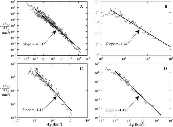
In the derivative method, we start with cumulative data, where N_CF is the number of forest fires with area greater than A_F. We define a noncumulative distribution in terms of the negative of the derivative of the cumulative distribution with respect to the area A_F. The value is negative, because the cumulative distribution is summed from the largest to the smallest values. A close approximation of the derivative, dN_CF/dA_F, is the slope of the best-fit line for a specified number of adjacent cumulative data points. Four forest fire data sets (8) have been converted to a noncumulative distribution and the results are given in Fig. 1. In each case the data are compared with the power-law relation

It is seen that the data correlate well with this relation taking exponent a_F = 1.3–1.5.

Fig 1.

Noncumulative frequency-area statistics for actual forest fires and wildfires in the United States and Australia (8). Four examples are given: (A) 4,284 fires on U.S. Fish and Wildlife Service land during 1986–1995, (B) 120 fires in the western United States during 1955–1960, calculated from tree ring data, (C) 164 fires in Alaskan Boreal Forests during 1990–1991, and (D) 298 fires in the Australian Capital Territory during 1926–1991. For each data set, the noncumulative number of fires per year, −dN_CF/dA_F, with area A_F, is given as a function of A_F. In each case a reasonably good correlation over many decades of A_F is obtained by using Eq. 4 with a_F = 1.3–1.5.

Considering the many complexities of the initiation and propagation of forest fires and wildfires, it is remarkable that the frequency-area statistics are very similar under a wide variety of environments. The proximity of combustible material varies widely. The behavior of a particular fire depends strongly on meteorological conditions. Firefighting efforts extinguish many fires. Despite these complexities, the application of power-law frequency-area distributions appears to be robust. Further confirmation of the applicability of the forest fire model to real forests is the observation that clusters of trees in forests obey power-law statistics (9).

It is of interest to determine whether the destruction of forests is dominated by the largest fires or the smallest fires. The total area of fires A_FT with areas less than A_F is given by

Substitution of Eq. 4 gives

As long as a_F < 2, the total area burned A_FT diverges as A_F → ∞. From Fig. 1 we see that this is the case for the forest fire data sets considered here. If linearly binned, the largest fires dominate in terms of the area burned.

Forest Fire Model

The scaling behavior of the forest fires illustrated above is very similar to the scaling behavior of the forest fire model (5, 6). In its simplest form, the forest fire model consists of a square grid of sites, with G the size of the grid. At each time step, a model tree is dropped on a randomly chosen site; if the site is unoccupied, the tree is planted. The sparking frequency f_s is the inverse number of attempted tree drops on the square grid before a model match is dropped on a randomly chosen site. If f_s = 1/100, there have been 99 attempts to plant trees (some successful, some unsuccessful) before a match is dropped at the 100th time step. If the match is dropped on an empty site, nothing happens. If it is dropped on a tree, the tree ignites and a model fire consumes that tree and all adjacent (nondiagonal) trees.

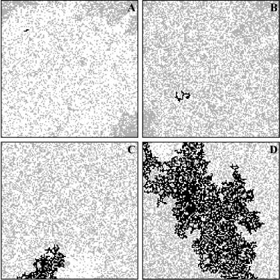
Having specified the size of the square grid G and the sparking frequency f_s, a simulation is run for N_S time steps and the number of fires N_F with area A_F is determined. The area A_F is the number of trees that burn in a fire. Examples of four typical model fires are given in Fig. 2. In this run, the grid size was 128 × 128 (G = 16,384), 1/f_s = 2,000, and fires with A_F = 5, 51, 506, and 5,327 trees are illustrated.

Fig 2.

Four examples of typical model forest fires are given for a 128 × 128 grid with sparking frequency 1/f_s = 2,000 (8). The heavily shaded regions are forest fires. The lightly shaded regions are unburned forest. The white regions are unoccupied sites. The areas A_F of the four forest fires are (A) 5, (B) 51, (C) 505, and (D) 5,327 trees. The largest forest fire is seen to span the entire grid.

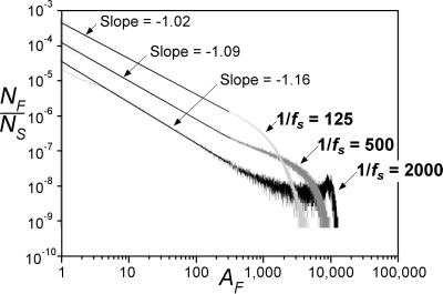
The noncumulative frequency-area distributions for the model forest fires are given in Fig. 3. The number of fires per time step with area A_F, N_F/N_S, is given as a function of A_F. Results are given for a grid size 128 × 128 and three sparking frequencies, 1/f_s = 125, 500, and 2,000. In all cases the smaller fires correlate well with the power-law relation, Eq. 3, with exponent a_F = 1.0–1.2.

Fig 3.

Noncumulative frequency-area distributions of model forest fires with constant grid size and changing sparking frequency (8). The number of fires per time step with size A_F, N_F/N_S, is given as a function of A_F, where A_F is the number of trees burned in each fire. Results are given for grid size 128 × 128 and sparking frequencies, 1/f_s = 125, 500, 2,000. For each f_s the model was run for N_S = 1.638 × 10⁹ time steps. The small and medium fires correlate well with Eq. 3 taking A_F = 1.02–1.18. At the smallest sparking frequency, 1/f_s = 2,000, fires begin to span the entire grid.

These results indicate the finite-size effect of the grid. If f_s is large, the frequency-area distribution begins to deviate significantly from a straight line, such that there is an upper termination to the power-law distribution. In Fig. 3, the deviation begins for 1/f_s = 125 and G = 128 × 128 at A_F ∼ 1,000. It is also seen that large fires become dominant when the sparking frequency is very small. This is easily explained on physical grounds and is illustrated in Fig. 3. With large sparking frequencies (e.g., 1/f_s = 125), fires occur before large clusters can form, and thus large fires rarely occur. For small sparking frequencies (e.g., 1/f_s = 2,000), large clusters form that can span the entire grid and large fires can occur.

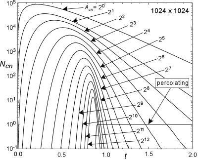
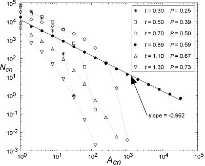
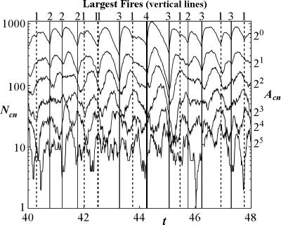
It is instructive to compare the forest fire model with the site-percolation model, which is known to exhibit critical behavior, as discussed below. The site-percolation model also consists of a square grid of sites and can be discussed in terms of forest fires (10). To compare the behavior of the site-percolation model with the forest fire model we consider the transient behavior of the forest fire model without any fires. Trees are planted on randomly chosen grid sites until the entire grid is filled with trees. The percolation threshold (critical point) is reached when a cluster of trees spans the grid (see Fig. 2D). The time evolution of the number of clusters of various sizes is given in Fig. 4. We use subscripts c for “cluster” and n for the logarithmic bin-size, A_cn = 2ⁿ; that is, N_c0 includes clusters of size 1, N_c1 clusters of size 2–3, N_c2 clusters of size 4–7, and so forth. The number of clusters of size A_cn, N_cn, is given as a function of time t. The unit of time, Δt = 1, represents G (i.e., the number of cells in the grid) attempts to plant trees. Initially, single-tree clusters, A_c0 = 2⁰, dominate; subsequently these grow and coalesce to form larger clusters of size 2¹, 2², 2³, and so forth. For the example given in Fig. 4, G = 1,024² and Δt = 1 represents 1,024² time steps. The process is a cascade from small to large clusters. The noncumulative frequency-area distributions of the logarithmically binned clusters from Fig. 4 are given in Fig. 5 for various times t.

Fig 4.

Dependence of the number of clusters, N_cn, of a specified size A_cn on time t for the forest fire model without any fires. Results are given for logarithmically binned clusters with N_cn being the number of clusters with area A_cn = 2ⁿ. For this example G = 1,024². One unit of time, Δt = 1.00, is equivalent to G attempts to plant trees.

Fig 5.

Frequency-area distributions of clusters for the forest fire model without any fires. The logarithmically binned number of clusters, N_cn, of size A_cn = 2ⁿ is given as a function of A_cn at various times, t, and corresponding probabilities, P. One unit of time, Δt = 1.00, is equivalent to G attempts to plant trees.

The continuous probability function P that a site is occupied by a tree is given by

where N_T is the number of trees on the grid. The critical probability (10) associated with percolation, P_c = 0.59275, is reached when t = 0.898. At this time, the logarithmically binned noncumulative frequency-area distribution given in Fig. 5 is well approximated by power-law exponent b_c = −0.96.

Although this transient problem clearly exhibits a cascade from small to large clusters, the resulting frequency-size distribution is only power law at the critical percolation threshold. At other times, when the density of trees is either less than or greater than the critical value P_c = 0.59275, the distribution deviates strongly from a power law (Fig. 5).

To illustrate the difference between critical and self-organized critical behavior we give an example of cluster size statistics for the forest fire model. Again, the clusters are logarithmically binned in sizes A_cn = 2ⁿ. With G = 128² and 1/f_s = 700, the number of binned clusters are given as a function of time in Fig. 6. The times at which large fires of various sizes occur are given as vertical straight lines. The numbers 1, 2, 3. and 4 represent fires that have a size between 10% and 20%, 20% and 30%, 30% and 40%, and 40% and 50% of the size of the grid, G. It is seen that large fires occur when clusters of size A_c1 and A_c2 are at a minimum. The growth and fall in numbers of small clusters is very similar to that illustrated in Fig. 4. After a large fire, the density of trees is low and there is a transient filling of empty sites. As the sites fill, the number of small clusters decrease until another major fire occurs. Although it is not possible to predict when large fires occur, it is seen that large fires do not occur when the numbers of small clusters is increasing.

Fig 6.

Dependence of the number of clusters, N_cn, of a specified size A_cn on time, t, for the forest fire model. Results are given for logarithmically binned clusters with N_cn being the number of clusters with area A_cn = 2ⁿ. For this example G = 128² and f_s = 1/700. One unit of time, Δt = 1.00, is equivalent to G attempts to plant trees. The vertical straight lines are large forest fires, the numbers 1–4 represent fires that have a size of between 10% and 20%, 20% and 30%, 30% and 40%, and 40% and 50% of the size of the grid, G.

A comparison of Figs. 5 and 6 illustrates some differences between self-organized criticality and criticality. For the forest fire model, the numbers of binned clusters fluctuate, but are well approximated by a power-law distribution at all times. The cascade of trees from small clusters to large clusters is continuous. The power-law (fractal) distribution of cluster sizes (and thus fire sizes) is a direct consequence of this continuous cascade.

The forest fire model without fires is identical to the site-percolation model. This model exhibits criticality and is a transient problem with the density of trees increasing in time until the grid is covered by trees. In the site-percolation model, power-law frequency-area distributions of tree clusters are found only near the critical value of the density of trees. This is the critical point and corresponds to the first cluster that spans the grid. In contrast, the forest fire model is a quasi steady-state model. Trees are continuously planted and continuously destroyed in model fires. The cascade of trees from small to large clusters results in a power-law frequency-size distribution for the clusters. This cascade behavior caused by the coalescence of tree clusters is a signature of self-organized critical behavior.

A rigorous definition of self-organized criticality is elusive, but a working definition is that the “input” to a complex system is nearly constant, whereas the “output” is a series of events or “avalanches” that follow a power-law (fractal) frequency-size distribution. Both the forest fire model and actual forest fires are examples of systems that have nearly constant input and an output (the fires) that follow robust power-law frequency-size distributions, despite many changes to the rules or parameters of the system. Thus, they might be systems that exhibit self-organized critical behavior.

Cascade Model

The scaling behavior of both the forest fire model and actual forest fires can be understood in terms of an inverse cascade model (11–13). This model is formulated in terms of individual trees on a grid and the clusters of trees that are generated. Individual trees are planted on the grid. A new tree can (i) create a new single-tree cluster, (ii) increase the size of an existing cluster by one if planted on a site immediately adjacent to the cluster, or (iii) bridge the gap between two clusters with n₁ and n₂ trees to form a new cluster with n₁ + n₂ + 1 trees. These three alternatives are illustrated in Fig. 7. Small clusters coalesce to form larger clusters. Individual trees cascade from smaller to larger clusters. Although clusters of all sizes coalesce with each other, the cascade is dominated by the coalescence of clusters of approximately equal size (13). Model fires destroy clusters of all sizes. But, we will show that the effects of the fires on the smaller clusters can be neglected.

Fig 7.

Different methods that clusters grow. The trees marked by x have been added. (A) A new single-tree cluster is formed. (B) A pre-existing cluster has been increased in size by one. (C) The gap between two pre-existing clusters has been bridged so that the two clusters have coalesced to form a single cluster.

To illustrate the behavior of the cascade model we will consider a simplified version. Trees will be introduced into the grid only as single-tree clusters. We again consider a logarithmically binned distribution of tree cluster sizes as described above. Coalescence will be assumed to be dominated by the combining of two clusters in the same logarithmic bin and the rate is given by a transition probability, C_n,n+1. We write a set of balance equations for N_cn, the number of tree clusters in a bin of size A_cn = 2ⁿ with the result

Eq. 8 is a balance equation for single tree clusters. The constant C₀ is the rate (trees per unit time) at which single-tree clusters are added to the cascade. The transition probability C_0,1 multiplied by N, the square of the number of tree clusters in a bin of size 2⁰, is the rate at which single trees A_c0 coalesce to form A_c1 clusters. Similarly, D₀N_c0 is the rate at which single tree clusters are lost in fires.

Eq. 9 is a balance equation for A_c1 clusters (2–3 trees). The term ½C_0,1N is the rate at which A_c1 clusters are formed from single trees; C_1,2N is the rate at which A_c1 clusters coalesce to form A_c2 clusters; and D₁N_c1 is the rate at which A_c1 clusters are lost in fires.

Eq. 10 is a balance equation for A_cn clusters. The term ½C_n−1,nN is the rate at which A_c,n−1 clusters coalesce to form A_cn clusters; C_n,n+1N is the rate at which A_cn clusters coalesce to form A_c,n+1 clusters; and D_nN_cn is the rate at which A_cn clusters are lost in fires.

The transition probability scales with N because each of the N_cn clusters can collide with the (N_cn − 1) other clusters and (N_cn − 1) ∼ N_cn because N_cn is large. We assume a power-law scaling of the coalescence transition probability on cluster area A_cn = 2ⁿ. We can then write:

where b_c is a positive constant.

The probability that a spark will hit a cluster of trees is proportional to the cluster area and number of clusters

where β is a positive constant. Substitution of n = 0, 1, (n − 1), and n into Eqs. 11 and 12, and these into Eqs. 8–10 gives

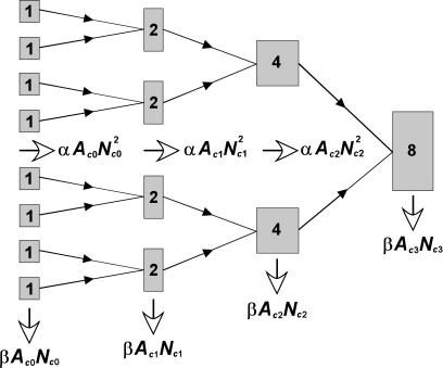
The behavior of this inverse cascade model is illustrated schematically in Fig. 8 for b_c = 1. Because the loss of clusters caused by coalescence scales with N, whereas the loss of clusters caused by fires scales with N_cn, the loss caused by fires can be neglected except in the largest clusters that terminate the cascade. Neglecting the N_cn fire loss terms in Eqs. 13–15, and taking the positive roots, we obtain

which can be generalized to give

As previously discussed, the power-law exponent b_c in a logarithmically binned noncumulative distribution of N_cn vs. A_cn is equivalent to the power-law exponent for the cumulative distribution, giving

where N_Cc is the (cumulative) number of clusters with area greater than or equal to A_c. We use A_c instead of A_cn, as the data set is now continuous (no longer logarithmically binned). In terms of the derivative of the cumulative distribution, Eq. 18 can be written as

because the noncumulative exponent a_c = b_c + 1. The scaling of the noncumulative distribution with an exponent follows directly from the choice of the exponent (2b_c − 1) in Eq. 11.

Fig 8.

Schematic flow diagram for the inverse-cascade model as it is applied to the forest fire model with a value for b_c = 1 in Eqs. 13–15. Two single tree clusters with area A_c0 = 2⁰ = 1 coalesce to form a cluster with A_c1 = 2¹. The cross section for coalescence is αA_c0N. Single-tree clusters are lost in fires at the rate βA_c0N_c0. This pattern repeats for higher-order clusters.

As discussed above, the number of fires of a given size dN_CF/dA_F is proportional to the number of clusters of that size dN_Cc/dA_c multiplied by that cluster's area A_c. Combining this with Eq. 19 gives

Because when a cluster of area A_c burns, it gives a fire of area A_F, the result in Eq. 20 is identical to Eq. 4 taking a_F = a_c − 1 = b_c. For the forest fire model with a_F = 1.0, we have a_c = 2.0 and b_c = 1.0; substitution into Eq. 11 gives C_n,n+1 ∼ A_cn. For actual forest fires with a_F = 1.4, we have a_c = 2.4 and b_c = 1.4; substitution into Eq. 11 gives C_n,n+1 ∼ A. The simple inverse cascade model developed in this section provides an explanation for the power-law frequency-area statistics for both the forest fire model and actual forest fires.

Landslides

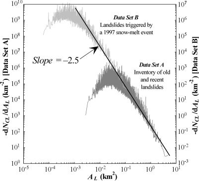
Landslides are another natural hazard that exhibits power-law frequency-area statistics under a wide variety of circumstances. We first consider a regional inventory of 16,809 landslides in the Umbria–Marche area of Italy (14). This inventory was obtained from analyses of aerial photographs taken at a 1:33,000 scale, supplemented by detailed geomorphic investigations at selected sites (15, 16). The noncumulative number-area distribution is given in Fig. 9 (data set A). The medium and large landslides correlate well with the power-law relation

with exponent a_L = 2.5 and intercept C = 300 (A_L in km²). This data set deviates from the power-law scaling for A_L < 10⁻¹ km² (A ≈ 300 m). The equivalent cumulative distribution for Eq. 21 is

We next consider an inventory of 4,233 landslides in the Umbria region that were triggered by a sudden change in temperature on January 1, 1997. This inventory was obtained from analyses of aerial photographs taken at a 1:20,000 scale 3 months after the snow-melt event, supplemented by field surveys. The noncumulative number-area distribution of these landslides is also given in Fig. 9 (data set B). Note that the vertical scales have been adjusted so that the two data sets overlap. These landslides also correlate well with the power-law relation in Eq. 21, again taking a_L = 2.5 and C = 0.3 (A_L in km²). This data set deviates from the power-law scaling for A_L < 10⁻³ km² (A ≈ 30 m).

Fig 9.

Noncumulative frequency-area distributions of central Italian landslides (14). The noncumulative frequency of landslides −dN_CL/dA_L with area A_L is given as a function of landslide area A_L for two data sets. Data set A represents an inventory of 16,809 old and recent landslides mapped in the Umbria–Marche area. Data set B represents 4,233 landslides triggered by a January 1997 rapid snow melting in Umbria.

The overlap of the two data sets illustrated in Fig. 9 shows that the power-law scaling is valid over the range of landslide areas, 10⁻³ km² < A_L < = 4 km², i.e., for lengths scales greater than A ≈ 30 m. The inventory of the snow-melt induced landslides (data set B) is certainly more complete than the historical landslides (data set A). We conclude that the rollover (at A_L = 2 × 10⁻² km² of the landslides in the regional inventory in data set A is caused by the inability to measure the areas of the smaller landslides on the aerial photographs and/or caused by erosion and other wasting processes.

On the other hand, the rollover of the landslides in data set B is not an artifact and is the result of the truncation of the power-law scaling at a length scale of about A ≈ 30 m. Because of the freshness of the snow melt-triggered landslides, and the quality and scale (1:20,000) of the aerial photographs, the smallest landslide area consistently mapped is about 2.5 × 10⁻⁴ km² (A ≈ 16 m), i.e., lower than the dimension A ≈ 30 m at which the data set deviates from the power-law relation. This conclusion also has been supported by detailed geomorphic investigations at selected sites, which confirmed that inventories from the aerial photographs are virtually complete.

The contribution of the snow melt-triggered landslides to the total landslide inventory also can be deduced from the comparison of data sets A and B in Fig. 9. In the actual landslide inventories, the snow melt-triggered landslides (data set B) have a total landslide area of 12.7 km² and represent 0.7% of the total landslide area of 1,831 km² of the long-term (regional) landslides (data set A). However, the frequency-area distributions as presented in Fig. 9 tell a different story. Assume that both inventories are complete for the larger landslides. Evidence that this is true can be seen in Fig. 9, where both data sets A and B have the same power-law distributions. Comparing the C value from Eq. 21 for both distributions (Fig. 9), data set B has C = 0.3 and data set A has C = 300; the ratio is 1:1,000.

The area under the two frequency-area distributions represents the relative total landslide area for each data set. Changing C in Eq. 21 by 1,000 is the same as changing the area under the frequency-area curve by a factor of 1,000. Therefore, based on the frequency-area distribution, the total area of the snow melt-triggered landslides (data set B) represents 0.1% of the total area of the long-term regional landslides (data set A). The lower value of 0.1% (vs. 0.7% as discussed in the last paragraph) is a reflection of the fact that data set A is incomplete.

An important question is the relative importance of triggered landslides in the long-term landslide inventory. Are most landslides generated in the largest triggered landslide events or is the landslide inventory dominated by the regular background of landslides? Certainly earthquakes, snow-melt events, and high intensity or prolonged rainfall events trigger many landslides. But what are the frequency-magnitude statistics for these events? The comparison made in Fig. 9 provides a rational basis for quantifying the intensity of a triggered landslide event. Simply taking the number of counted landslides is inappropriate; doing this for the comparison given in Fig. 8 would lead to a serious error, as data set B is relatively complete (i.e., all or a large percentage of the triggered landslides are counted) and A is incomplete. Based on the actual landslide inventories, the relative intensities of the two data sets would be 4,233/16,809 or ≈1/4. This is very different from our previous conclusion based on the power-law distribution for each data set, and the ratio 1:1,000 for the values of C, that the relative intensities are 1/1,000.

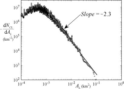
For comparison, we now consider the frequency-area distribution of 10,000 landslides triggered over an area of 10,000 km² by the January 17, 1994, Northridge, CA earthquake. An inventory of these landslides was carried out by Harp and Jibson (17). They used 1:60,000 scale aerial photography, taken the morning after the earthquake, and compared these photos with photos taken previously. The digitized photos were supplemented by fieldwork. They estimated that the inventory is nearly complete for landslides with a length scale greater than A ≈ 5 m. The noncumulative number-area distribution of these landslides is given in Fig. 10. These landslides correlate well with the power-law relation Eq. 21 taking a_L = 2.3 and C = 1.0 (A_L in km²). This data set deviates from the power-law scaling for A_L < 10⁻³ km² (A ≈ 30 m).

Fig 10.

Noncumulative frequency-area distribution of 11,000 landslides triggered by the January 17, 1994, Northridge, CA earthquake (17). The noncumulative frequency of landslides −dN_CL/dA_L with area A_L is given as a function of landslide area A_L.

The data for these earthquake-triggered landslides in California are remarkably similar to the snow melt-triggered landslides in central Italy. The best-fit power-law exponent is a_L = 2.3 for the California data and a_L = 2.5 for the Italian data. The rollovers for small landslides occur at essentially the same landslide areas for the two data sets. The relative intensities of the snow melt-triggered landslides can be obtained from the correlations given in Figs. 9 and 10. A comparison made at A_L = 10⁻² km² shows that the intensity of the California landslide event was about twice the intensity of the Italian landslide event. Because both inventories appear to be relatively complete, the relative intensities are proportional to the number of landslides, i.e., 11,000/4,233 = 2.6.

We next compare the results given above with previous studies. Fujii (18) obtained a cumulative number-area inventory of 800 landslides caused by a heavy rainfall event in Japan. An excellent correlation with the power-law relation Eq. 22 was found, taking b_L = 0.96. The equivalent noncumulative power-law exponent in Eq. 21 is a_L = 1.96. Hovius et al. (19) have given a number-area inventory of 4,984 landslides in the montane zone east of the Alpine fault in New Zealand. They estimated that these landslides occurred over a 40- to 60-year period. Their logarithmically binned data correlated well with a power-law relation with exponent b_L = 1.17. Because logarithmic binning is equivalent to a cumulative distribution (Eq. 22), the equivalent noncumulative power-law exponent from Eq. 21 is a_L = 2.17.

Hovius et al. (20) have given a number-area inventory of 1,040 fresh landslides in the Ma-An and Wan-Li catchments on the eastern side of the Central Range in Taiwan. They estimated the landslides have an age of less than 10 years. Their logarithmically binned data had a power-law exponent of b_L = 1.66. The equivalent noncumulative power-law exponent from Eq. 21 is a_L = 2.66. This data set deviates from the power-law scaling for A_L < 10⁻³ km² (A ≈ 30 m). It is interesting to note that the power-law exponent and the deviation from power-law scaling for this data set and the two landslide events we gave above (Italy and California) are very similar.

Noncumulative number-area distributions for several regional landslide inventories have been given by Malamud and Turcotte (21). Results for 1,130 landslides from the Challana Valley, Bolivia correlate well with the noncumulative power-law relation, Eq. 21, taking a_L = 2.6; 3,243 landslides from the Akishi Range, central Japan correlate well, taking a_L = 3.0; and 709 earthquakes from Eden Canyon, Alameda, CA correlate well, taking a_L = 3.3.

Hungr et al. (22) have given cumulative frequency-volume inventories for 1,937 rock falls and rock slides along the main transportation corridors of southwestern British Columbia. The data correlate reasonable well with a power-law relation taking the slope to be −0.5 ± 0.2. Assuming the volume V correlates with the area according to V ∼ A^3/2, the equivalent cumulative frequency-area power-law exponent (Eq. 22) is b_L = 0.75 ± 0.30, and the equivalent noncumulative frequency-area power-law exponent (Eq. 21) is a_L = 1.75 ± 0.30.

Dai and Lee (23) have given cumulative frequency-volume inventories for 2,811 landslides in Hong Kong that occurred during the period 1992–1997. The data correlate reasonably well with a power law taking the slope to be −0.8. Again assuming V ∼ A^3/2, the equivalent cumulative frequency-area power-law exponent (Eq. 22) is b_L = 1.2, and the equivalent noncumulative frequency-area power-law exponent (Eq. 21) is a_L = 2.2.

Although there is certainly variability, many landslide inventories appear to satisfy noncumulative power-law frequency-area statistics with an exponent a_L = 2.5 ± 0.5. An important question is whether this relatively large scatter in values of a_L is caused by scatter in the data or by different values of a_L associated with different geology. For a single data set, the error bar on a_L can be relatively large. For instance, depending on where the tail is fit, Stark and Hovius (24) find variations on the order of a_L = 2.88 ± 0.22. This variation is also quiet evident in our Fig. 9, where for each data set an error bar of a_L = 2.5 ± 0.25 is reasonable. But, when the two data sets are combined, the error is reduced to a_L = 2.5 ± 0.10. This combination suggests that the power-law distribution of landslides may be valid over a wider range of values than shown by previous studies.

We believe the evidence is convincing that medium and large landslides consistently satisfy power-law (fractal) frequency-area statistics, but why? One explanation is to simply invoke the sand pile model as an analog for landslides in the same way that slider-block models are associated with earthquakes. However, the noncumulative power-law exponent for landslides is a_L = 2.5 ± 0.5 whereas the noncumulative power-law exponent for the sand pile model avalanches is a_L ∼ 1.0. To explain this difference, Pelletier et al. (25) combined a slope stability analysis with self-affine topography and soil-moisture content and found a power-law noncumulative frequency-area distribution with a_L = 2.6.

Hergarten and Neugebauer (26) used a numerical model combining slope stability and mass movement and found an approximation to a power-law distribution with an exponent of a_L ∼ 2.1. These authors (27) later used a cellular-automata model with time-dependent weakening, similar to the sand pile model, and found a power-law distribution with a_L ∼ 2.0. Although it is certainly possible to develop models that reproduce the observed power-law dependence of actual data, there is a real question whether these models are realistic in terms of the governing physics. Certainly much more work is required to provide a comprehensive explanation for the power-law behavior.

The rollover of the data away from the power-law correlation for small landslides also appears to be systematic and requires an explanation. One possibility is that the rollover scale has a geomorphological explanation. The rollover occurs for scales less than about 30 m, the scale on which well-defined stream networks form. The gullying associated with stream and river networks would be expected to play a significant role in the geometry of landslides for climatically controlled failures, such as those of data set B, or other landslides triggered by rainfall. For climatically controlled landslides, water and groundwater are important issues and both relate to the size of a slope, which in turn depends on the pattern and density of the river network. For seismically induced landslides, the relationship is less clear. These landslides, and particularly rock falls, occur where slopes are steeper, where seismic shaking concentrates, and where the rock is weaker. An alternative explanation for the rollover of the data are that this scale represents a transition from failures controlled by cohesion to failures controlled by basal friction.

Conclusions

The evidence is clear that the three natural hazards—earthquakes, forest fires, and landslides—are complex phenomena that self-organize under a wide variety of conditions. In each case the frequency-area statistics are power law over a wide range of scales. This “fat-tail” behavior has important implications regarding the occurrence of large events. Large events are much more likely to occur if the tail is “fat,” i.e., power law, than if it is “thin,” i.e., exponential.

An inverse cascade model can explain the power-law scaling region. This model is directly applicable to forest fires. Clusters of flammable trees grow in size as new trees result in the coalescence of smaller clusters to form larger clusters. Significant numbers of trees are lost only in the largest fires that terminate the cascade of trees from small clusters to large clusters. The cluster coalescence is self-similar, leading to a power-law distribution of cluster sizes.

This cascade model can also be used to explain the scaling of earthquakes and landslides. As the tectonic stress in a region increases the metastable areas over which an earthquake can spread grow by coalescence. Significant metastable areas are lost only in the largest earthquakes. The metastable regions where landslides can occur grow because of mountain building processes. This growth occurs by the coalescence of smaller metastable regions. The landslides occur in these metastable regions caused by a triggering event, i.e., an earthquake, a snow-melt event, a rain event. In both cases, the scale invariant cascade of clusters leads directly to a power-law distribution.

References

- 1.Gutenberg B. & Richter, C. F., (1954) Seismicity of the Earth and Associated Phenomenon (Princeton Univ. Press, Princeton).
- 2.Aki K. (1981) in Earthquake Prediction, eds. Simpson, D. & Richards, P. (Am. Geophys. Union, Washington, DC), pp. 566–574.
- 3.Burridge R. & Knopoff, L. (1967) Seis. Soc. Am. Bull. 57, 341-371. [Google Scholar]
- 4.Carlson J. M. & Langer, J. S. (1989) Phys. Rev. A At. Mol. Opt. Phys. 40, 6470-6484. [DOI] [PubMed] [Google Scholar]
- 5.Bak P., Chen, K. & Tang, C. (1992) Phys. Lett. A 147, 297-300. [Google Scholar]
- 6.Drossel B. & Schwabl, F. (1992) Phys. Rev. Lett. 69, 1629-1632. [DOI] [PubMed] [Google Scholar]
- 7.Bak P., Tang, C. & Wiesenfeld, K. (1988) Phys. Rev. A At. Mol. Opt. Phys. 38, 364-374. [DOI] [PubMed] [Google Scholar]
- 8.Malamud B. D., Morein, G. & Turcotte, D. L. (1998) Science 281, 1840-1842. [DOI] [PubMed] [Google Scholar]
- 9.Sole R. V. & Manrubia, S. C. (1995) Phys. Rev. E Stat. Phys. Plasmas Fluids Relat. Interdiscip. Top. 51, 6250-6253. [DOI] [PubMed] [Google Scholar]
- 10.Stauffer D. & Aharony, A., (1992) Introduction to Percolation Theory (Taylor & Francis, London).
- 11.Turcotte D. L., Malamud, B. D., Morein, G. & Newman, W. I. (1999) Physica A 268, 629-643. [Google Scholar]
- 12.Turcotte D. L. (1999) Rep. Prog. Phys. 62, 1377-1429. [Google Scholar]
- 13.Gabrielov A., Newman, W. I. & Turcotte, D. L. (1999) Phys. Rev. E Stat. Phys. Plasmas Fluids Relat. Interdiscip. Top. 66, 5293-5300. [DOI] [PubMed] [Google Scholar]
- 14.Guzzetti, F., Malamud, B. D., Turcotte, D. L. & Reichenbach, P. (2002) Earth Planet Sci. Lett., in press. [DOI] [PMC free article] [PubMed]
- 15.Guzzetti F., Carrarra, A., Cardinali, M. & Reichenbach, P. (1999) Geomorphology 31, 181-216. [Google Scholar]
- 16.Guzzetti F., Cardinali, M. & Reichenbach, P. (1996) Environ. Eng. Geol. 2, 531-555. [Google Scholar]
- 17.Harp E. L. & Jibson, R. L., (1995) U.S. Geological Survey Open File Report 95–213 (U.S. Geological Society, Washington, DC).
- 18.Fujii Y. (1969) J. Seismol. Soc. Japan 22, 244-247. [Google Scholar]
- 19.Hovius N., Stark, C. P. & Allen, P. A. (1997) Geology 25, 231-234. [Google Scholar]
- 20.Hovius N., Stark, C. P., Hao-Tsu, C. & Jinn-Chuan, L. (2000) J. Geol. 108, 73-89. [DOI] [PubMed] [Google Scholar]
- 21.Malamud B. D. & Turcotte, D. L. (1999) Natural Hazards 20, 93-116. [Google Scholar]
- 22.Hungr O., Evans, S. G. & Hazzard, J. (1999) Can. Geotechnol. J. 36, 224-238. [Google Scholar]
- 23.Dai F. C. & Lee, C. F. (2001) Eng. Geol. 59, 253-266. [Google Scholar]
- 24.Stark C. P. & Hovius, N. (2001) Geophys. Res. Lett. 28, 1091-1094. [Google Scholar]
- 25.Pelletier J. D., Malamud, B. D., Blodgett, T. & Turcotte, D. L. (1997) Eng. Geol. 48, 255-268. [Google Scholar]
- 26.Hergarten S. & Neugebauer, H. J. (1998) Geophys. Res. Lett. 25, 801-804. [Google Scholar]
- 27.Hergarten S. & Neugebauer, H. J. (2000) Phys. Rev. E Stat. Phys. Plasmas Fluids Relat. Interdiscip. Top. 61, 2382-2385. [Google Scholar]