Natural variability of atmospheric temperatures and geomagnetic intensity over a wide range of time scales

Abstract

The majority of numerical models in climatology and geomagnetism rely on deterministic finite-difference techniques and attempt to include as many empirical constraints on the many processes and boundary conditions applicable to their very complex systems. Despite their sophistication, many of these models are unable to reproduce basic aspects of climatic or geomagnetic dynamics. We show that a simple stochastic model, which treats the flux of heat energy in the atmosphere by convective instabilities with random advection and diffusive mixing, does a remarkable job at matching the observed power spectrum of historical and proxy records for atmospheric temperatures from time scales of one day to one million years (Myr). With this approach distinct changes in the power-spectral form can be associated with characteristic time scales of ocean mixing and radiative damping. Similarly, a simple model of the diffusion of magnetic intensity in Earth's core coupled with amplification and destruction of the local intensity can reproduce the observed 1/f noise behavior of Earth's geomagnetic intensity from time scales of 1 (Myr) to 100 yr. In addition, the statistics of the fluctuations in the polarity reversal rate from time scales of 1 Myr to 100 Myr are consistent with the hypothesis that reversals are the result of variations in 1/f noise geomagnetic intensity above a certain threshold, suggesting that reversals may be associated with internal fluctuations rather than changes in mantle thermal or magnetic boundary conditions.

In this paper we consider the power spectrum of temporal variations in atmospheric temperature on time scales of 10⁻² to 10⁶ yr. The spectral behavior for time scales between 200 thousand years (kyr) and 500 yr is obtained from deuterium concentrations in the Vostok ice core. Historical temperature records are analyzed to give the spectral behavior between time scales of 100 yr and 1 day. The obvious daily and annual periodicities are removed, and we focus on the stochastic content of the time series. We show that at frequencies smaller than f ≈ 1/(40 kyr), the power spectrum is flat (white noise). At frequencies between f ≈ 1/(40 kyr) and f ≈ 1/(2 kyr), the power spectrum is proportional to f⁻² (a Brownian walk). At frequencies greater than f ≈ 1/(2 kyr), the power spectrum is proportional to f^−1/2. At very high frequencies [above f ≈ 1/(1 month)], the spectrum varies as f^−3/2 for continental stations and remains proportional to f^−1/2 for maritime stations. Solutions to a stochastic diffusion equation for a two-layer system representing the coupled atmosphere–ocean reproduce the observed statistics. This system was first studied in the context of semiconductor physics. The observed power spectrum of atmospheric temperature is identical to the power spectrum of variations caused by the stochastic diffusion of heat in a metallic film that is in thermal equilibrium with a substrate (1). Temperature variations in the film and substrate occur as a result of fluctuations in the heat transport by electrons undergoing Brownian motion. The top of the film absorbs and emits blackbody radiation. In our analogy, we associate the atmosphere with the metallic film and the oceans with the substrate. Turbulent eddies in the atmosphere and oceans are analogous to the electrons undergoing Brownian motion in a metallic film in contact with a substrate.

In addition to considering climate variability, we also consider variations in the intensity of Earth's magnetic field. Earth's magnetic field has exhibited significant variability over a wide range of time scales. On time scales less than a couple of hundred years, historical data are available for variations in the intensity and orientation of the geomagnetic field. Archeomagnetic data can be used to infer the intensity of the field from time scales of centuries to millenia. Sediment cores provide the widest range of time scales of variations in the geomagnetic field with internal origin: 1 kyr to 10 million years (Myr). Techniques of time series analysis can be used to characterize this variability. The geomagnetic field also exhibits reversals with a complex history including variations over a wide range of time scales. The reversal history can be characterized by the polarity interval distribution and the reversal rate. Polarity intervals vary from those short enough to be barely resolved in the magnetic anomalies of the seafloor to the 35-Myr Cretaceous superchron. Reversals are also clustered in time such that short polarity intervals tend to be followed by short polarity intervals and long intervals by long intervals. This clustering has been quantified with the reversal rate, which gradually decreases going back to 100 mega-annum (Ma) and then increases going back further in time before the Cretaceous superchron.

We perform power-spectral analyses of time series data for the intensity of Earth's magnetic field inferred from sediment core and archeomagnetic data. We find that the power spectrum of the intensity of the geomagnetic field from time scales of 100 yr to 10 Myr is well approximated by a 1/f dependence, where f is the frequency. Variations in the intensity of the geomagnetic field in one polarity exhibit a normal distribution. When a fluctuation crosses the zero intensity value a reversal occurs. We test the hypothesis that reversals are the result of intensity variations with a 1/f power spectrum, which occasionally are large enough to cross the zero intensity value, driving the geodynamo into the opposite polarity state. Synthetic time series with a 1/f power spectrum and a binormal distribution are used to generate reversal statistics. These are found to be in good agreement with those of the real reversal history, suggesting that intensity variations and reversals of the magnetic field are a natural consequence of the inherent variability generated by dynamo action and magnetic diffusion in the core. A model that generates the observed 1/f behavior is a two-dimensional stochastic diffusion equation.

Power-Spectral Analysis of Atmospheric Temperature Variations

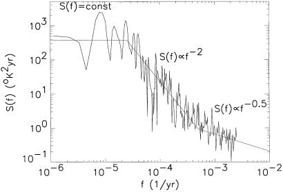
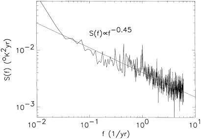
We first consider the spectral behavior of the deuterium concentrations in the Vostok (East Antarctica) ice core. A 220-kyr record of temperature fluctuations is obtained by using the conversion 5.6 δD(%) = 1°K (2). Jouzel and Merlinvat (3) have concluded that the Vostok deuterium record is a proxy for local atmospheric temperature. Because the data are unevenly sampled we utilized the Lomb periodogram (4) to estimate the power spectrum. The results are given in Fig. 1. We associate the power spectrum with three regions of different self-affine behavior. The first region, at frequencies less than f ≈ 1/(40 kyr), is a white noise [S(f) is constant]. The second region, between f ≈ 1/(40 kyr) and f ≈ 1/(2 kyr), is a Brownian walk [S(f) ∝ f⁻²]. In the third region, with frequencies greater than f ≈ 1/(2 kyr), there is a change to a lower absolute value the power-spectral exponent [S(f) ∝ f^−1/2]. This change is associated with more rapid variations in the Vostok core at short time scales. This is also observed in ice cores from Greenland (5). Several authors have reported the low-frequency behavior (a flat spectrum crossing over to f⁻² behavior) with other paleoclimatological data (6, 7). To extend our analyses to higher frequencies we have carried out power-spectral analyses on data for atmospheric temperature variations from weather stations. We have determined the average power spectrum of the time series of monthly mean temperatures from 94 stations worldwide with the yearly trend removed. We obtained the power spectra S(f) of all complete temperature series of length greater than or equal to 1,024 months from the climatological data base compiled by Vose et al. (8). The yearly trend was removed by subtracting from each monthly data point the average temperature for that month in the 86-yr record for each station. All of the power spectra were then averaged at equal frequency values. The results are given in Fig. 2. The data yield a straight line on a log–log plot with slope close to −½ indicating that S(f) ∝ f^−1/2 in this frequency range.

Fig 1.

Power-spectral density estimated with the Lomb periodogram of the temperature inferred from the deuterium concentrations in the Vostok (East Antarctica) ice core. The power-spectral density S is given as a function of frequency for time scales of 500 yr to 200 kyr.

Fig 2.

Average power-spectral density of 94 complete monthly temperature time series from the data set of Vose et al. (8) plotted as a function of frequency in yr⁻¹. The power-spectral density S is given as a function of frequency for time scales of 2 months to 100 yr.

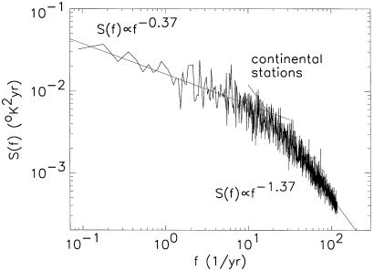
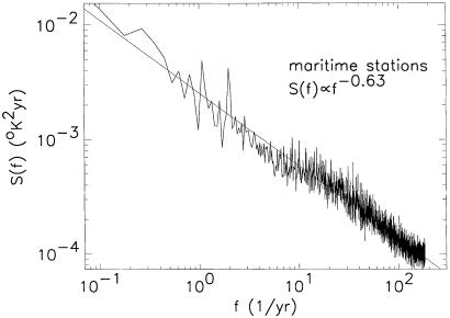
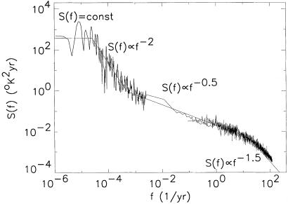
Finally, we consider the average power spectrum of time series of daily mean temperature (estimated by taking the average of the maximum and minimum temperature of each day) from 50 continental and 50 maritime stations over 4,096 days. Maritime stations are sites on small islands far from any large land masses. Continental stations are well inland on large continents, far from any large bodies of water. We chose 50 stations at random from the complete records (those with greater than 4,096 nearly consecutive days of data) provided by the Global Daily Summary database compiled by the National Climatic Data Center (9). Once again, the yearly periodicities were removed. The results are given in Figs. 3 and 4. Continental stations (Fig. 3) correlate with an f^−3/2 high-frequency region. Maritime stations (Fig. 4) correlate with an f^−1/2 scaling up to the highest frequency. The crossover frequency for the continental spectra is f ≈ 1/(1 month). The difference between continental and maritime stations results from the air mass above maritime stations exchanging heat with both the atmosphere above and the oceans below, whereas the air mass above continental stations exchanges heat only with the atmosphere above it. The three spectra have been combined in Fig. 5 to give a continuous spectral behavior of local atmospheric temperature from frequencies of 10⁻⁶ to 10² yr⁻¹.

Fig 3.

Average power-spectral density of 50 continental daily temperature time series from the data set of the National Climatic Data Center (9) as a function of frequency in yr⁻¹. The power-spectral density S is given as a function of frequency for time scales of 2 days to 10 yr.

Fig 4.

Average power-spectral density of 50 maritime daily temperature time series from the data set of the National Climatic Data Center (9) as a function of frequency in yr⁻¹. The power-spectral density S is given as a function of frequency for time scales of 2 days to 10 yr.

Fig 5.

Power-spectral density of local atmospheric temperature from instrumental data and inferred from ice cores from time scales of 200 kyr to 2 days. The high frequency data are for continental stations. Piecewise power-law trends are indicated.

We can interpret these results in terms of the vertical turbulent transport of heat energy in the atmosphere in addition to its radiation into space and its exchange with the ocean. The ocean acts as a thermal reservoir, buffering changes in atmospheric temperature. In our model, vertical turbulent transport is modeled as a stochastic diffusion process. Convective instabilities diffuse heat energy within the atmosphere by turbulent mixing. Deterministic diffusion is not adequate to model atmospheric heat transport, however, because the stochastic nature of turbulent flow in the atmosphere gives rise to fluctuations in the transport of heat through time. Therefore, it is appropriate to model turbulent transport by the diffusion equation with a random noise in the flux term:

where J is the heat flux, ΔT is the fluctuation in temperature from equilibrium, ρ is the density, c is the heat capacity per unit mass, σ is the thermal conductivity, and η is a Gaussian white noise in space and time. Eq. 1 is conservation of energy. Eq. 2 is Fourier's law of heat transport with random advection of heat superimposed. The noise term is chosen to be Gaussian white noise because velocity fluctuations in atmospheric turbulence are observed to be Gaussian and white above a time scale of minutes.

We now determine the behavior of the stochastic diffusion model in terms of the power spectrum of temperature fluctuations in a layer of width 2l. We consider an infinite space in which 1 and 2 are applicable. We focus our attention on a layer of width 2l in this space. The presentation we give is similar to that of Voss and Clarke (10). The variations in total heat energy in the layer of width 2l is determined by the heat flow across the boundaries. A diffusion process has a frequency-dependent correlation length λ = (2α/f)^1/2 (10), where α is the diffusion coefficient α = σ/(ρc). Two different situations arise as a consequence of the length scale, 2l, of the geometry. For high frequencies λ ≪ 2l the fluctuations in heat flow across the two boundaries are independent. For low frequencies λ ≫ 2l and the fluctuations in heat across the two boundaries are in phase.

First we consider high frequencies. Because the boundaries fluctuate independently, we can consider the flow across one boundary only. The flux of heat energy is given by Eq. 2. Its Fourier transform is given by

where f = 2πω, and k is the wave number. The flux of heat energy out of the layer at the boundary at x = l (the other boundary is located at x = −l) is the rate of change of the total energy in the layer E(t): dE(t)/dt = J(l, t). The Fourier transform of this equation is

Therefore, the power spectrum of variations in E(t), S_E(ω) = 〈|E(ω)|²〉 is

In the above expression, the noise term η does not appear because it is white noise in space and time; it's average amplitude is independent of ω and k, i.e., it is just a constant. Because ΔT ∝ ΔE, the power spectrum of temperature has the same form as S_E and S_T(ω) ∝ ω^−3/2.

If we include the heat flux out of both boundaries, the rate of change of energy in the layer will be given by the difference in heat flux: dE(t)/dt = J(l, t) − J(−l, t). The Fourier transform of E(t) is now

Then,

where θ = (ω/ω_o)^1/2, and ω_o = α/2l² is the frequency where the correlation length is equal to the width of the layer. When λ ≪ 2l, the above expression reduces to S_T(f) ∝ f^−3/2. When λ ≫ 2l, S_T(f) ∝ f^−1/2 (10). In this limit the boundaries fluctuate in phase, and heat that enters into the region from one boundary can diffuse out of the other boundary. The result is a sequence of fluctuations that are less persistent than the single boundary f^−3/2 case.

In the introduction, we presented evidence that continental stations exhibit an f^−3/2 high-frequency region, and maritime stations exhibit f^−1/2 scaling up to the highest frequency considered. This observation can be interpreted in terms of the diffusion model presented above. The power spectrum of temperature variations in an air mass exchanging heat by one-dimensional stochastic diffusion is proportional to f^−1/2 if the air mass is bounded by two diffusing regions and is proportional to f^−3/2 if it interacts only with one. The boundary conditions appropriate to maritime and continental stations are a layer interacting with two (upper atmosphere and ocean) and one (upper atmosphere only) thermal reservoirs, respectively. The layer considered is taken to have an upper boundary embedded in the atmosphere and a lower boundary at the earth's surface. For maritime stations, heat is transferred across this lower boundary into the oceans so it is equivalent to the case λ/l > 1 and therefore the power spectrum of temperature variations is S(f) ∝ f^−1/2. For continental stations, the lower boundary is insulating so it is equivalent to the case λ/l < 1 and therefore S(f) ∝ f^−3/2. At low frequencies, horizontal heat exchange between continental and maritime air masses limits the variance of the continental stations. This crossover occurs at the time scale when the air masses above continents and oceans become mixed. The time scale for one complete Hadley or Walker circulation which mixes the air masses is approximately 1 month, the same time scale as the observed crossover.

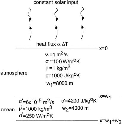
Next we consider the stochastic diffusion model in a geometry appropriate for a coupled atmosphere–ocean model with an atmosphere of uniform density (equal to the density at sea level) in thermal contact with oceans of uniform density. The height of our model atmosphere is the scale height of the atmosphere (height at which the pressure falls by a factor of e from its value at sea level). Fig. 6 illustrates the geometry and constants chosen with σ as the vertical heat conductivity, ρ as the density, c as the specific heat per unit mass, α as the vertical thermal diffusivity, and g as the thermal conductance of heat out of the Earth by emission of radiation. Primed constants denote values for the oceans. The physical constants that enter the model are the density, specific heat, vertical thermal diffusivity, depths of the oceans and atmosphere, and the thermal conductance by emission of radiation. The density and specific heat of air and water are well known constants. We chose an ocean depth of 4 km and an atmospheric height equal to the scale height of 8 km. The eddy diffusivity we use for the oceans is 6 × 10⁻⁵ m²/s. This value has been obtained from Tritium dispersion studies (11). The vertical eddy diffusivity for the atmosphere we use is 1 m²/s, as quoted by Pleune (12) and Seinfeld (13) for stable air conditions. This eddy diffusivity implies an equilibration time of the tropospheric air column to be 2 years. This value is roughly consistent with the 1-yr vertical mixing time of the Pinatubo and El Chichon aerosols (14, 15).

Fig 6.

Geometry of the coupled atmosphere–ocean model and the constants chosen.

The equation for temperature fluctuations in space and time in the model is

The mean value of η is zero and the flux of heat of proportional to the temperature:

The delta functions indicate that the white noise term η is uncorrelated in space and time.

The boundary conditions are that no heat flows out of the bottoms of the oceans and continuity of temperature and heat flux at the atmosphere–ocean boundary:

At the top of the atmosphere we impose a blackbody radiation boundary condition. Most (65%) of the energy incident on the Earth is reradiated as long-wavelength blackbody radiation from the H₂O and CO₂ in the atmosphere (16). This radiated energy depends on the temperature of the atmosphere at the point of emission according to the Stefan–Boltzmann law. It is common practice to assume that temperature variations about equilibrium are small. This is a good approximation because the global mean temperature has fluctuated by only about 10 degrees K during the last glaciation. With a linear approximation, the radiated energy is proportional to the temperature difference from equilibrium (17). The boundary condition at the scale height of the atmosphere (which we take to be representative of the average elevation where radiation is emitted from the atmosphere) is then

We will use the value g = 1.7 W/m²°K as used by Ghil (17) and Harvey and Schneider (18).

The existence of two layers of different diffusivity makes the study of the two-layer model much more complex than for the one-layer models applied to the atmosphere above the continents and the oceans. Van Vliet et al. (1) used Green's functions to solve this two-layer model. The Green's function of the Laplace-transformed diffusion equation is defined by

where G is governed by the same boundary conditions as ΔT. This equation can be solved by separating G into two parts: G_a and G_b with x < x′ and x > x′, respectively. G_a and G_b satisfy the homogeneous (unforced) diffusion equation with a jump condition relating G_a and G_b:

The power spectrum of the average temperature in the atmosphere in terms of G is given by Van Vliet et al. (1) as:

where G₁ stands for the solution to the differential equation for G where the source point is located in the atmosphere, and Re denotes the real part of the complex expression. Two forms of G_1a and G_1b are necessary for x located above and below x′, respectively, because of the discontinuity in the derivative of G₁ created by the delta function. The solution of G₁, which satisfies the above differential equation and boundary conditions, is

and

where

and L = (α/iω)^1/2 and L′ = (α′/iω)^1/2. Performing the integration Van Vliet et al. (1) obtained

For very low frequencies several approximations can be made:

Reducing this equation,

This is the low-frequency Lorentzian spectrum observed in the Vostok data. The crossover frequency as a function of the constants chosen for the model is

At high frequencies the following approximations hold

then

This is the broad f^−1/2 region observed in the power spectrum of the temperature data and predicted based on the simpler one-layer model exchanging heat with regions above and below. The high- and low-frequency spectra meet at

This value agrees within an order of magnitude to that observed in the Vostok data [f ≈ 1/(2 kyr)].

The three crossover time scales in the composite spectrum of Fig. 5 are fundamental time scales of the climate system. The 1-month time scale for crossover between f^−3/2 and f^−1/2 behavior in continental stations can be associated with the time scale for horizontal mixing between air masses over the continents with air masses over adjacent oceans.

For time scales greater than 1 month but less than 2 kyr, fluctuations in out-going heat energy from the atmosphere by radiative cooling causes temperature variations in the atmosphere that can be damped by the oceans. At frequencies lower than 2 kyr, the time scale of vertical ocean mixing, the atmosphere, and oceans are in thermal equilibrium. The oceans can no longer absorb thermal fluctuations in the atmosphere resulting from fluctuations in radiative emission at this time scale. The variance in temperature of the atmosphere and oceans is then determined solely by the radiation boundary condition. The fluctuating temperature at the top of the atmosphere will result in a white noise flux out of the atmosphere–ocean system. The average temperature of the atmosphere and oceans at these time scales will be given by the sum of a white noise, a Brownian walk. This is observed in the Vostok data between time scales 2–40 kyr.

The power spectrum of temperature variations flattens out at frequencies lower than f ≈ 1/(40 kyr) as a result of a negative feedback mechanism: as the coupled atmosphere and oceans warm up (cool down) because of nonstationary fluctuations resulting from the random heat flux out into space, the system will radiate, on average, more (less) radiation, limiting the variance at low frequencies. This can be described by a linear damping equation for the global temperature difference from equilibrium:

where τ_o = 1/f_o and f_o is given by (2.27). The temperature variations ΔT from this equation have a spectrum that is a Lorentzian with a crossover time scale of τ_o. This can be shown with Fourier transforms. The Fourier transform of Eq. 32 is given by

The power spectrum S_ΔT(ω) = 〈|ΔT(ω)|²〉 is then given by Eq. 25. Now we must consider whether the observed low-frequency crossover time scale of 40 kyr is consistent with the model prediction given by

If we neglect the heat capacity of the atmosphere relative to that of the ocean, this reduces to

The first term is the time scale for radiative damping of the heat energy of the coupled atmosphere–ocean system into space. The second term is the time scale for transport of the heat energy of the ocean to the top of the atmosphere where it can be radiated from clouds. If the time scale for one of these processes is much larger than the time scale for the other, the crossover time scale will be determined by that rate-limiting step. For the Earth's climate system, the transport of the oceans' heat through the atmosphere seems to be the rate-limiting step. This process takes a long time because the atmosphere has a low heat capacity compared to the oceans and is therefore a poor heat conductor. The time scale of radiative damping is estimated to be 600 yr from the well known constants listed in Fig. 6. The time scale for vertical transport of the oceans' heat through the atmosphere can be estimated to only within an order of magnitude because this time scale linearly depends on the average vertical diffusivity of the atmosphere. Only rough estimates are available for this parameter. Estimates of 1 m²/s for this parameter have been given by Pleune (12) and Seinfeld (13). For the time scale of vertical advection of the oceans' heat through the atmosphere to be 40 kyr, a vertical diffusivity of 0.1 m²/s is required, a factor of 10 lower but roughly in agreement with the values quoted above.

Manabe and Stouffer (19) have completed power-spectral analyses of variations in local atmospheric temperature in control runs of a coupled atmosphere–ocean–land surface model. They computed the power spectrum of temperature time series of each surface grid point and then averaged the power spectra at equal frequency values, as in our observational power-spectral analyses. They found different spectra for continental and maritime gridpoints. Maritime gridpoints exhibited power-law power spectra from time scales of 1 month to several hundred years with an exponent of close to −0.25. Continental gridpoints, however, showed flat spectra up to time scales of about 100 yr, in contrast to observations.

Variability of Earth's Magnetic Field

In this section we consider the time series of Earth's magnetic field. Paleomagnetic studies show clearly that the polarity of the magnetic field has been subject to reversals. Kono (20) has compiled paleointensity measurements of the magnetic field from volcanic lavas for 0–10 Ma. He concluded that the distribution of paleointensity is well approximated by a symmetric binormal distribution with mean 8.9 × 10²² Am² and standard deviation 3.4 × 10²² Am². A normal distribution is applicable to the field when it is in its normal polarity and the other when it is in its reversed polarity.

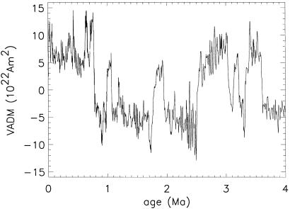
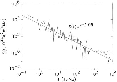
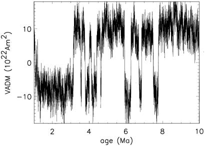
We have utilized three data sets for computing the power spectrum of the dipole moment of the earth's magnetic field. They are archeomagnetic data from time scales of 100 yr to 8 kyr from Kovacheva (21), marine sediment data from the Somali basin from time scales of 1 kyr to 140 kyr from Meynadier et al. (22), and marine sediment data from the Pacific and Indian Oceans from 20 kyr to 4 Myr from Meynadier et al. (23). The data were published in table form in Kovacheva and obtained from L. Meynadier (personal communication) for the marine sediment data in Meynadier et al. (22, 23). Marine sediment data are accurate measures of relative paleointensity but give no information on absolute intensity. To calibrate marine sediment data, the data must be compared to absolute paleointensity measurements from volcanic lavas sampled from the same time period as the sediment record. Meynadier et al. (23) have done this for the composite Pacific and Indian Oceans data set. They have calibrated the mean paleointensity in terms of the virtual axial dipole moment for 0–4 Ma as 9 × 10²² Am² (24). This value is consistent with that obtained by Kono (20) for the longer time interval up to 10 Ma. By using this calibration, we calibrated the Somali data with the time interval 0–140 ka from the composite Pacific and Indian Oceans dataset. The data from Meynadier et al. (23) are plotted in Fig. 7 as a function of age in Ma. The last reversal at approximately 730 thousand years BP (Ka) is clearly shown. We computed the power spectrum of each of the time series with the Lomb periodogram (4). The compiled spectra are given in Fig. 8. The composite sediment record from the Pacific and Indian Oceans are plotted up to the frequency 1/(25 kyr). Above this time scale good synchroneity is observed in the Pacific and Indian Oceans data sets by Meynadier et al. (23). This suggests that nongeomagnetic effects such as variable sedimentation rate are not significant in these cores above this time scale. From frequencies of 1/(25 kyr) to 1/(1.6 kyr) we plot the power spectrum of the Somali data. From time scales of 1.6 kyr to the highest frequency we plot the power spectrum of the data of Kovacheva. A least-squares linear regression to the data yields a slope of −1.09 over 4.5 orders of magnitude. This indicates that the power spectrum is well approximated as 1/f on these time scales.

Fig 7.

Paleointensity of the intensity of Earth's magnetic field as inferred from sediment cores for the past 4 Ma from Meynadier et al. (23). The data are expressed as the virtual axial dipole moment (VADM) with reversed polarity data given by negative values.

Fig 8.

Power spectrum of the geomagnetic field intensity variations estimated with the use of the Lomb periodogram from sediment cores of Meynadier et al. (22, 23) and archeomagnetic data from Kovacheva (21). The power spectrum S is given as a function of frequency f for time scales of 100 years BP to 4 Ma.

The power spectrum of secular geomagnetic intensity variations has been determined to have a 1/f² power spectrum between time scales of 1 and 100 years (25–27). This is consistent with the analysis of McLeod (28) who found that the first difference of the annual means of geomagnetic field intensity is a white noise because the first difference of a random process with power spectrum 1/f² is a white noise. Our observation of 1/f power-spectral behavior above time scales of approximately 100 yr together with the results of Currie (25) and Barton (26) suggests that there is a crossover from 1/f to 1/f² spectral behavior at a time scale of approximately 100 years.

Analysis of the Polarity Reversal Record and Relationship to Paleointensity Variations

We will now show that the statistics of the reversal record are consistent with those of a binormal 1/f noise paleointensity record, which reverses each time the intensity crosses the zero value. We will compare the polarity length distribution and the clustering of reversals between synthetic reversals produced with 1/f noise intensity variations and the reversal history.

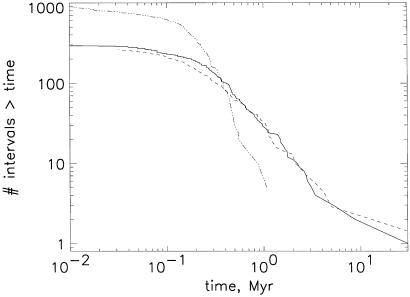
First we consider the polarity length distribution of the real reversal history. The polarity length distribution calculated from the chronology of Harland et al. (29) is given as the solid line in Fig. 9. The polarity length distribution is the number of interval lengths longer than the length plotted on the horizontal axis. A reassessment of the magnetic anomaly data has been performed by Cande and Kent (30, 31) to obtain an alternative magnetic time scale. The polarity length distribution of their time scale normalized to the same length as the Harland et al. time scale, is presented as the dashed curve. The two distributions are nearly identical. These plots suggest that the polarity length distribution is better fit by a power law for large polarity lengths than by an exponential distribution, as first suggested by Cox (32). The same conclusion has been reached by Gaffin (33) and Seki and Ito (34).

Fig 9.

Cumulative frequency-length distribution of the lengths of polarity intervals during the last 170 Ma from the time scale of Harland et al. (29) (solid curve), Cande and Kent (30, 36) (dashed curve), and the Cande and Kent (30, 36) time scale from C1 to C13 with cryptochrons included (dashed and dotted line).

The third curve, plotted with a dashed-dotted line, represents the polarity length distribution estimated from the magnetic time scale between C1 and C13 with “cryptochrons” included and scaled to the length of the Harland et al. (29) time scale. Cryptochrons are small variations recorded in the magnetic anomaly data that may either represent variations in paleomagnetic intensity or short reversals (35, 36). Cryptochons occur with a time scale at the limit of temporal resolution of the reversal record from magnetic anomalies of the sea floor. The form of the polarity length distribution estimated from the record between C1 and C13 including cryptochrons is not representative of the entire reversal history because of the variable reversal rate that concentrates many short polarity intervals in this time period. However, this distribution enables us to estimate the temporal resolution of the reversal record history. The distribution estimated from C1 to C13 has many more short polarity intervals than those of the full reversal history starting at a reversal length of 0.3 Myr. Above a time scale of 0.3 Myr the magnetic time scale is nearly complete. Below it, many short polarity intervals may be unrecorded.

To show that this distribution is consistent with binormal 1/f noise intensity variations, we have generated synthetic Gaussian noises with a power spectrum proportional to 1/f, a mean value of 8.9 × 10²² Am², and an SD of 3.4 × 10²² Am² as obtained by Kono (20), representative of the field intensity in one polarity state. To construct a binormal intensity distribution from the synthetic normal distribution, we inverted every other polarity interval to the opposite polarity starting from its minimum value below the zero intensity axis and extending to its next minimum below the zero. The result of this procedure on the Gaussian, 1/f noise of Fig. 10 is presented in Fig. 11. Its irregular polarity lengths are similar to those in the marine sediment data of Fig. 7.

Fig 10.

A binormal 1/f noise constructed from a 1/f noise with a mean of 8.9 × 10²² Am² and an SD of 3.4 × 10²² Am² representing the geomagnetic field intensity (VADM) in one polarity state. The binormal noise was then constructed by multiplying the intensity values of every second interval between zero crossings by −1 to create a binormal distribution.

Fig 11.

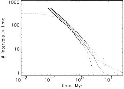
Cumulative frequency-length polarity interval distributions from the Harland et al. (29) time scale and that of the binormal 1/f noise model of intensity variations. The distribution from the Harland et al. time scale (dashed curve) was also given in Fig. 9. The solid line represents the average cumulative distribution from the 1/f noise model. The dotted lines represent the minimum and maximum reversal length distributions for 20 numerical experiments, thereby representing 95% confidence intervals.

The operation of reversing the paleomagnetic intensity when it crosses the zero intensity value is consistent with models of the geodynamo as a system with two symmetric attracting states of positive and negative polarity such as the Rikitake disk dynamo. Between reversals, the geomagnetic field fluctuates until a fluctuation large enough occurs to cross the energy barrier into the other basin of attraction.

We have computed the distributions of lengths between successive reversals for 20 synthetic noises scaled to length 169 Ma, the length of the reversal chronology, and averaged the results in terms of the number of reversals. The results are plotted as the solid curve along with the Harland et al. (29) time scale (dashed curve) in Fig. 11. The dots in Fig. 11 are the maximum and minimum values obtained in the 20 synthetic reversal chronologies for each reversal rank, thus representing 95% confidence intervals. The synthetic polarity length distribution matches that of the Harland et al. time scale within the 95% confidence interval over all time scales plotted except for the Cretaceous superchron, which lies slightly outside of the 95% confidence interval, and reversals separated by less than about 0.3 Myr. The overprediction of very short reversals could be a limitation of the model or a result of the incompleteness of the reversal record for short polarity intervals. As mentioned, the temporal resolution of the magnetic time scale inferred from magnetic anomalies is approximately 0.3 Myr. We conclude that the polarity length distribution produced from binormal 1/f intensity variations is consistent with the observed polarity length distribution for all time scales for which the reversal record is complete.

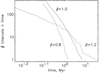
We next consider whether the agreement illustrated in Fig. 11 is unique to 1/f noise. We have computed polarity length distributions by using binormal intensity variations with power spectra f^−0.8 and f^−1.2. These results along with the 1/f result from Fig. 10 are given in Fig. 12. The shape of the polarity length distribution is very sensitive to the exponent of the power spectrum. A slight increase in the magnitude of the exponent results in many more long polarity intervals than with 1/f noise. We conclude that the agreement in Fig. 12 between the synthetic reversal distribution and the true reversal history is unique to 1/f noise and provides strong evidence that the dipole moment has 1/f behavior up to time scales of 170 Myr.

Fig 12.

Cumulative frequency-length polarity interval distributions for the 1/f noise model of intensity variations (shown in the middle, also given in Fig. 5) and for intensity variations with power spectra proportional to f^−0.8 and f^−1.2. This plot illustrates that the polarity length distribution is very sensitive to the form of the power spectrum, allowing us to conclude that the agreement between the model and the observed distribution is unique to 1/f noise intensity variations.

A binormal, 1/f noise geomagnetic field variation is consistent with the qualitative results of Pal and Roberts (37) who found an anticorrelation between reversal frequency and paleointensity. This anticorrelation is evident in the synthetic 1/f noise of Fig. 11. During the time intervals of greatest average paleointensity the reversal rate is lowest.

It is generally believed that secular geomagnetic variations are the results of internal dynamics whereas longer time scale phenomena such as variations in the reversal rate are controlled by variations in boundary conditions at the core–mantle boundary (CMB) (38). Variations in mantle activity have been proposed as the driving force for reversals (39). However, our observation of continuous 1/f spectral behavior from time scales of 100 yr to 170 Myr suggests that internal variability may control variations in geomagnetic intensity over the entire range of time scales analyzed here.

Conclusions

At frequencies below about 1/(40 kyr), the noise spectrum of atmospheric temperature is flat (white noise). Radiative transfer from the atmosphere is balanced against the solar input. At frequencies between about 1/(40 kyr) and 1/(2 kyr), the global temperature drifts and is a Brownian walk. The oceans and atmosphere act as a single thermal bath that is not buffered by radiative losses to infinity. At frequencies between about 1/(2 kyr) and 1/(1 month), the atmospheric temperature is stationary and is well approximated by a self-affine behavior with a power-law power spectrum with exponent of −½. In this frequency range, the atmospheric temperature is buffered by heat exchange with the oceans, which act as a near-isothermal bath. At frequencies between about 1/(1 month) and 1/(1 day), the temperatures at continental stations again drift, and are well approximated by a nonstationary self-affine behavior with an exponent of −, whereas maritime stations remain with an exponent of −½. The maritime stations are buffered by the oceanic heat sink, whereas the continental stations are not.

We also considered the temporal variability of Earth's magnetic field. By combining a variety of paleointensity measurements, we are able to obtain the power spectrum of the dipole moment of the field over the frequency range 1/(4 Myr) to 1/(100 yr). Over this entire range, the power spectrum is well approximated by a 1/f self-affine time series.

As a further test of this result we considered the field's reversal record. We produced synthetic 1/f time series with the observed mean and variance of Earth's magnetic field. Each time a synthetic field reached zero field intensity, we assumed that the polarity of the field was changed. We then compared the statistics of the synthetic fields with the observed statistics. Good agreement was found.

Even though the dynamo driving the earth's magnetic field is extremely complex, the statistical behavior of the resulting magnetic-field time series is quite simple. This simplicity must be one of the primary tests for the validity of new dynamo theories.

Abbreviations

• Myr, million years

• kyr, thousand years

• Ma, mega-annum

References

- 1.Van Vliet K. M., van der Ziel, A. & Schmidt, R. R. (1980) J. Appl. Phys. 51, 2947-2956. [Google Scholar]
- 2.Jouzel J., Lorius, C., Petit, J. R., Genthon, C., Barkov, N. I. & Kotlyakov, V. M. (1987) Nature (London) 329, 403-407. [Google Scholar]
- 3.Jouzel J. & Merlivat, D. (1984) J. Geophys. Res. 89, 11749-11757. [Google Scholar]
- 4.Press W. H., Teukolsky, S. A., Vetterling, W. T. & Flannery, B. P., (1992) Numerical Recipes in C: The Art of Scientific Computing (Cambridge Univ. Press, New York).
- 5.Yiou P., Jouzel, J., Johnsen, S. & Rognvaldsson, O. E. (1995) Geophys. Res. Lett. 22, 2179-2182. [Google Scholar]
- 6.Hasselmann K. (1971) Tellus 6, 473-485. [Google Scholar]
- 7.Komintz M. A. & Pisias, N. G. (1979) Science 204, 171-172. [DOI] [PubMed] [Google Scholar]
- 8.Vose R. S., Schmoyer, R. L., Stewer, P. M., Peterson, T. M., Heim, R., Karl, T. R. & Eischeid, J. K., (1992) The Global Historical Climatology Network: Long-Term Monthly Temperature, Precipitation, Sea-Level Pressure, and Station Pressure Data. (Oak Ridge National Laboratory, Oak Ridge, TN), Envir. Sci. Div. Pub. No. 392.
- 9.National Climatic Data Center, (1994) Global Daily Summary: Temperature and Precipitation 1977–1991 (NCDC, Asheville, NC), Version 1.0.
- 10.Voss R. F. & Clarke, J. (1976) Phys. Rev. B 13, 556-573. [Google Scholar]
- 11.Garrett A. E. (1984) J. Mar. Res. 42, 359-393. [Google Scholar]
- 12.Pleune R. (1990) Atm. Env. A 24, 2547-2555. [Google Scholar]
- 13.Seinfeld J. H., (1986) Atmospheric Chemistry and Physics of Air Pollution (Wiley, New York). [DOI] [PubMed]
- 14.Hofmann D. J. & Rosen, J. M. (1987) J. Geophys. Res. 92, 9825-9830. [Google Scholar]
- 15.Rosen J. M., Kjome, N. T., McKenzie, R. T. & Liley, J. B. (1994) J. Geophys. Res. 99, 25733-25739. [Google Scholar]
- 16.Peixoto J. P. & Oort, A. H., (1992) Physics of Climate (Am. Inst. Phys., New York).
- 17.Ghil M., (1983) Turbulence and Predictability in Geophysical Fluid Dynamics and Climate Dynamics (North Holland, Amsterdam).
- 18.Harvey L. D. D. & Schneider, S. H. (1985) J. Geophys. Res. 90, 2191-2205. [Google Scholar]
- 19.Manabe S. & Stouffer, R. J. (1996) J. Climate 9, 376-393. [Google Scholar]
- 20.Kono M. (1971) Earth Plan. Sci. Lett. 11, 10-17. [Google Scholar]
- 21.Kovacheva M. (1980) Geophys. J. R. Astr. Soc. 61, 57-64. [Google Scholar]
- 22.Meynadier L., Valet, J.-P., Weeks, R., Shackleton, N. J. & Hagee, V. L. (1992) Earth Plan. Sci. Lett. 114, 39-57. [Google Scholar]
- 23.Meynadier L., Valet, J.-P., Bassonot, F. C., Shackleton, N. J. & Guyodo, Y. (1994) Earth Plan. Sci. Lett. 126, 109-127. [Google Scholar]
- 24.Valet J.-P. & Meynadier, L. (1993) Nature (London) 366, 234-238. [Google Scholar]
- 25.Currie R. G. (1968) J. Geophys. Res. 73, 2779-2768. [Google Scholar]
- 26.Barton C. E. (1982) Philos. Trans. R. Soc. London A 306, 203-209. [Google Scholar]
- 27.Courtillot V. & LeMouel, J. L. (1988) Annu. Rev. Earth Planet. Sci. 16, 389-476. [Google Scholar]
- 28.McLeod M. G. (1992) J. Geophys. Res. 97, 17261-17290. [Google Scholar]
- 29.Harland W. B., Cox, A., Llewellyn, P. G., Pickton, C. A. G., Smith, A. G. & Walters, R., (1990) A Geologic Time Scale 1989 (Cambridge Univ. Press, New York).
- 30.Cande S. C. & Kent, D. V. (1992) J. Geophys. Res. 97, 13917-13951. [Google Scholar]
- 31.Cande S. C. & Kent, D. V. (1995) J. Geophys. Res. 100, 6093-6095. [Google Scholar]
- 32.Cox A. (1968) J. Geophys. Res. 73, 3247-3260. [Google Scholar]
- 33.Gaffin S. (1989) Phys. Earth Plan. Int. 57, 284-290. [Google Scholar]
- 34.Seki M. & Ito, K. (1993) J. Geomag. Geoelectr. 45, 79-88. [Google Scholar]
- 35.Blakely R. J. (1974) J. Geophys. Res. 79, 2979-2985. [Google Scholar]
- 36.Cande S. C. & Kent, D. V. (1992) J. Geophys. Res. 97, 15075-15083. [Google Scholar]
- 37.Pal P. C. & Roberts, P. H. (1988) Nature (London) 331, 702-705. [Google Scholar]
- 38.McFadden P. L. & Merrill, R. T. (1995) J. Geophys. Res. 100, 307-316. [Google Scholar]
- 39.Larson R. L. & Olson, P. (1991) Earth Plan. Sci. Lett. 107, 437-447. [Google Scholar]