Short-memory traders and their impact on group learning in financial markets

Abstract

This article highlights several issues from simulating agent-based financial markets. These all center around the issue of learning in a multiagent setting, and specifically the question of whether the trading behavior of short-memory agents could interfere with the learning process of the market as whole. It is shown in a simple example that short-memory traders persist in generating excess volatility and other features common to actual markets. Problems related to short-memory trader behavior can be eliminated by using several different methods. These are discussed along with their relevance to agent-based models in general.

There is little controversy that learning and adaptation play a role in economic and social systems. Just what role learning plays and how it enters into either helping or hurting both the decision-making of individuals, and groups, and obtaining their goals is still a major question. This article presents some examples from agent-based financial markets to show that group learning and social self-organization can be tricky in many situations. It also demonstrates that there may be some common issues related to the learning process of adaptive agents both in financial markets and other settings.

The key issue for learning in agent-based models is that the players face a constantly changing environment made up of their fellow players and their respective strategies. A super rational learning world would have players trying to carefully second-guess the moves of all others while trying to out-maneuver them. Agent-based markets replace this framework with one of individuals following relatively simple behavioral rules that are updated over time. Therefore, although they are far from all-knowing, these participants are still learning and trying to do the best they can in what might be an ever-changing environment.

There are many reasons for moving to the boundedly rational world of agent-based models. First, the computational requirements of keeping track of everyone else in a financial market setting are probably enormous and out of the reach of anyone. Second, it seems to be the case that most individual behavior is based on simple “rules of thumb” rather than complicated deductive logic. Finally, complex rules in many situations may not be robust to small mistakes. The potential mispecifications and mistakes made by complicated rules in capturing the world may lead to their eventual demise.†

The key issue for learning in an agent-based world is that individuals must learn while other market participants are learning as well. The environment that they are trying to learn about is most likely changing over time, as other behaviors change. The changing endogenous heterogeneity of the population greatly affects a person's ability to figure out what to do. This obvious aspect of social systems can make learning a simple market situation difficult and can lead to interesting dynamics, which in some cases do a good job of replicating time series from actual markets.

Another crucial part of the learning process presented here is time. It is not surprising, given that change plays an important role in these markets, that time will also be a critical feature. In a changing world agents must take some stand on how they view the past. If learning requires some data points from the past, then the question of how far back into the past the learner should go needs to be answered. For someone believing that the world is stationary the answer to this question is pretty easy. He or she should use all available information. However, if one views the world as constantly in a state of change, then it will be better to use time series reaching a shorter length into the past. In the computer experiments presented here, this question will generally be left to an evolution. In other words, long-memory agents, using lots of past data, will be pitted against short-memory agents to see who takes over the market.

A final time issue that will be touched on here is the speed of learning. The actual rate at which agents learn turns out to a critical feature in many settings. At first it might seem that learning as often as possible would be the best strategy to follow, but we will see that this is often not the case, which is an interesting nonintuitive result from the agent-based modeling world.

This article uses a simple agent-based financial market as a computational example for the points mentioned earlier. Several things make financial markets an interesting place to apply these techniques. They produce rich data sets with many outstanding puzzles that still lack sufficient explanation. They also might be a system where evolutionary fitness can be reasonably connected to something that is easily observable—financial wealth. Finally, on the theoretical side, financial economics has viewed markets as being in an equilibrium where learning has uncovered most of what needs to be known. Agents are simply fine-tuning their models with prices well represented by a common, and agreed on, pool of financial knowledge. Recently, efficient markets concepts have been questioned by the growing following of behavioral economics, which stresses potential psychological biases and less than optimal behavioral rules of participants.‡ Actually, a key foundation of the efficient markets hypothesis has been one based on evolution and survival. The idea is that badly performing trading strategies will be driven out of a market, leaving only a stable set of optimal, well learned behaviors.§ Unfortunately, this evolutionary argument is wrong. The problem goes back to the coevolutionary ideas presented previously. Agent strategy performance is determined by those around the agents, not by a static finance benchmark selecting poor performers from good. Although it is possible convergence to some type of equilibrium can and will occur, convergence depends critically on the economic setting and the learning dynamics occurring within it.

Market Description presents a short outline of the model that will be used in the discussions. Computational Experiments describes the key results and their implications for the issues mentioned above. Finally, Summary and Conclusions will conclude and make some conjectures about agent modeling in the future.

Market Description

The market simulations used here are part of the class of economic models referred to as “agent-based.” Models of this type consist of large numbers of interacting agents each acting independently of the others often with active learning and adaptation.¶ Agent-based markets share many features, such as many interacting individuals, evolutionary dynamics, learning, and bounded rationality. However, the key distinguishing feature is that heterogeneity itself is endogenous. Markets can move through periods that support a diverse population of beliefs, and others where these beliefs and strategies might collapse down to a very small set.

The market description presented here is short. More detailed descriptions can be found in refs. 20 and 21. The market is a very simple one with a single equity-like security paying a random dividend each period and available in a fixed supply of one. This dividend follows a stochastic growth process that is calibrated to aggregate dividend series for the U.S. There is a risk-free asset that is available in infinite supply paying a constant real interest rate of zero. Portfolios are rebalanced, and trades are made at a monthly frequency. Also, prices are determined, and dividends are paid each month, which can be thought of as the basic unit of time in the market. Therefore, this is more of an experiment concerned with longer-term macroeconomic behavior as opposed to the minute by minute dynamics of day trading.

The market is populated with 500 agents. The agents sign on to certain investment strategies that can be viewed as mutual funds or investment advisors. They are represented by artificial neural networks that map current market information into a portfolio recommendation, which is the fraction of the portfolio to be invested in stocks. This value is constrained to be between zero and one, which excludes short selling and borrowing to purchase stock. The strategy takes as inputs common financial information such as dividend price ratios, current and lagged returns, and two moving average technical indicators. The latter compare the price to a moving average of past prices and are a common strategy used by investors in actual markets.

The strategies are evolved over time by using a genetic algorithm. Fitness is determined simply by whether a strategy has anyone using it. Unused strategies are discarded, and those in use can play the role of parents for evolving new strategies for the future. The genetic algorithm is specially modified to consider the specific structure of the neural network. When a new rule is created it must report a complete record of its performance as though it had existed in the past. However, it does differ from the real world where new mutual funds can often start with a clean slate in terms of past performance.

The most crucial aspect of the market is the method by which agents select strategies. They have well defined preferences over consumption each period given by

They consume a constant fraction of wealth and choose a strategy to maximize their expected logarithm of returns coming from the dynamic strategy.∥ To estimate this objective, they must use some amount of past data. The amount to use is part of the agent's own description. Some will be long-memory types, and will use many years' worth of returns from the past to evaluate rules. Others will be short-memory types, who consider only the recent past in their decisions. The objective function for traders is given by

The function α(z_t) represents the dynamic strategy as a function of past information. The value T_i indicates the number of past periods to use in choosing an optimal rule. The key issue here is when, if ever, do the long-memory types drive out the short-memory types.

Trading between the agents takes place every period. Given the strategies, aggregate demand is a well defined nonlinear function. The market is cleared nonlinearly to balance the demand for shares with the aggregate supply of one share. After the price is determined, the dividend is paid, agents' consumption is recorded, and the market moves on to the next period.

Computational Experiments

Benchmarks.

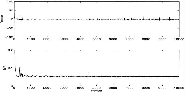
Fig. 1 displays the results of a market simulation consisting of traders with many different memory lengths. They are drawn from a uniform distribution between 6 months and 20 years. Log Price displays the log of the price series, which should have a linear trend driven by the constant dividend growth. This trend is evident in the figure, but the prices seem to take large deviations around this trend. Volume displays the trading volume in units of shares traded. Because there is one share in total, a volume of 0.1 would correspond to trading in one-tenth of the total shares outstanding. Volume is not a large fraction of the shares outstanding (most often it is below 5%). However, it is not going to zero as it should if the agents' beliefs were converging to each other. Returns shows the returns that also demonstrate some features of actual markets. There are large spikes corresponding to large up and down moves in the market. This movement corresponds to the well documented nongausseineity of financial return series. Also, the volatility in the market seems to be clumped with periods of relative calm and periods of large activity. All of these are features of actual market returns and are documented in further detail (20). D/P (dividend–price ratio) compares the movements of the equity price series with its underlying fundamental. This graph displays the annualized D/P. This value should be a constant if there were no changes in the underlying riskiness of the equity security, but it is clear from the figure that large and persistent deviations occur in this simulated market.

Fig. 1.

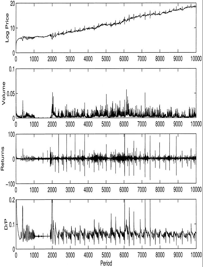
Heterogeneous memory. Price, trading volume, returns, and D/P ratio (annualized) for agent memory 0.5–20 years.

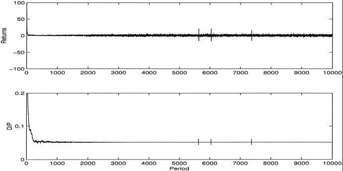
All these facts would be interesting on their own, but the purpose of this article is to test their sensitivity to changes in the basic assumptions. The first, and most critical, change is to require the population of agents to be long memory. Fig. 2 presents results of an experiment restricting the agents' memory lengths to be between 16–20 years. For comparison, the plots are presented on the same scales as Fig. 1. The conjecture being tested is that much of the variability, and instability, in the market is coming from the presence of short-memory traders. Fig. 2 generally confirms this feature. The price series is much more stable. Trading volume is near zero except for a few brief jumps. Returns are also generally stable with the exception of a few jumps, and finally the D/P ratio is very close to constant.

Fig. 2.

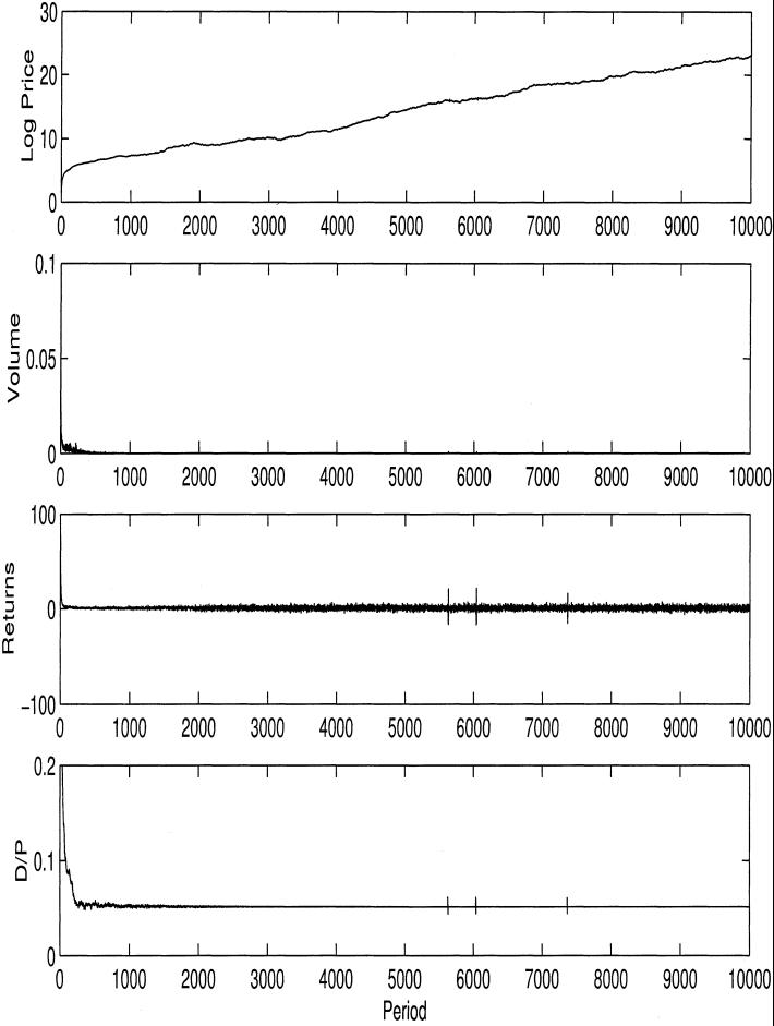
Homogeneous memory. Price, trading volume, returns, and D/P ratio (annualized) for agent memory 17–20 years.

The values in these figures can be determined theoretically. Estimates show that the market is approaching the theoretical benchmark of a well defined homogeneous agent equilibrium. Two important features should be noted. First, the agents are not told what this equilibrium is initially, thus in the early stages of the run the agents are actively learning their behavior. This learning leads to the brief levels of trading volume during the earliest periods. Second, the market is not perfect in its behavior in the equilibrium. Agents who are using stochastic learning algorithms will occasionally try unusual strategies, but these do not lead to large deviations from the equilibrium. These dynamics reveal information about the stability properties of the equilibrium in a multiagent environment.

These results show a market capable of generating two very different outcomes. One displays results looking closer to actual financial data, and the second with only long-memory agents reveals series that are close to a textbook market equilibrium. The following section explores changing several other parameters that will drive the market in either direction. The parameters are chosen to have some intuitive connection to understanding what may be hampering social learning in the heterogeneous agent case.

Slow Learning and Frictions.

In the previous cases, half the agents are chosen at random to reevaluate their rules. Results such as those in (2) suggest that the speed with which adaptation is occurring may be critical to the results. The experiments in Fig. 3 present cases where learning is slowed. The fraction of agents adjusting their rules each period is reduced to 0.05 from 0.5 in the previous experiments. At this much slower learning rate the dynamics change dramatically. It is clear from the figure that the deviations of the D/P ratio are very small, and the returns series is much less volatile and no longer shows the large spikes.

Fig. 3.

Slow learning. Returns and D/P ratio.

Because this slowing of the learning process is somewhat arbitrary, the next experiment is to use a more economic approach in terms of adding frictions. Fig. 4 takes the heterogeneous agent population used in Fig. 1 and adds a threshold to changing rules, which can be viewed as a kind of “switching cost,” although it is not exactly a cost of switching rules nor is it exactly a transaction cost. It is in the spirit of trying to throw some frictions into the system to slow things down. In these experiments agents change rules only when the new rule beats the old one by a given threshold of 10%. For example, if an agent uses a strategy that generates annual returns of 5%, a replacement strategy would have to do better than 5.5%, which is probably close to what agents would have to consider if they were facing true transaction costs, and it also would be consistent with requiring some kind of statistical threshold before changing rules.

Fig. 4.

Switching costs. Returns and D/P ratio.

Fig. 4 displays the returns and D/P ratios for a threshold run. The figures reveal a market much closer to the homogeneous long-memory case although the agent set is again drawn from 6 months to 20 years. The presence of a threshold on switching has slowed learning down enough that the agents were able to coordinate and learn their way into the equilibrium. It is surprising that adding some frictions yields a better performing market. This is a very nonintuitive result for an economic model. However, it has some connections to the policy proposals of implementing a transaction tax on trading, often referred to as a Tobin tax.

Summary and Conclusions

Individual agent learning in socioeconomic settings should not be viewed in isolation. That others are adapting strategies too leads to a coevolutionary dynamical system with many interesting features. The cause of much of this interesting dynamics can be related to the interaction between learners with differing views of the past. Agents with a short-term perspective can both influence the market in terms of increasing volatility, and create a evolutionary space where they are able to thrive.

These results contrast sharply with the commonly held wisdom in finance that “bad” strategies will eventually be driven out of the market. The problem with this argument is that weakly performing strategies are measured relative to the current population set and not some arbitrary stationary yardstick. It is this feature that is at the core of heterogeneous agent models and their coevolutionary nature. These experiments go one step further in trying to find out which aspects of the market are keeping it from converging. Obviously, changing the population to more long-memory types leads to a reliable convergence in strategies, which is a useful benchmark test. However, modifying other parameters can also have a crucial impact. Slowing rule changes either by directly controlling the fraction of the population updating rules or by introducing frictions also causes the population to converge. This result is slightly nonintuitive, because it would seem that imposing arbitrary frictions on trade or agent decision-making should hinder market performance. A population of slower decision makers actually does better than faster-thinking ones. There may be some interesting connections from this to other aspects of coevolution in economic and technological systems where dependencies across people and goods are great. Slowing things down may stop a kind of fruitless adaptation against an objective that is changing so fast that optimization is impossible.

In the early construction of agent-based models we are looking for many things. Obviously, extensive validation and testing will be an important part of the process, along with comparisons with experimental results. However, agent simulations alone can give a small or large nudge to traditional theorizing in some cases. For financial markets it is important to realize that evolutionary arguments for market efficiency are not robust. Also, it would seem that very simple forms of irrationality, such as short-memory behavior, might not be easily driven out of a market, which suggests that in the multiagent learning world, some forms of suboptimal, if not irrational, learning may persist for quite some time. Also, these models may yield further counter-intuitive results in terms of methods to stabilize, predict, or improve on current market institutions.

Abbreviations

• D/P, dividend–price ratio

References

- 1.Bookstaber R. (1999) Financ. Anal. J. 55, 18-20. [Google Scholar]
- 2.Axelrod R., (1984) The Evolution of Cooperation (Basic Books, New York).
- 3.Lindgren K. (1992) in Artificial Life II, eds. Langton, C. G., Taylor, C., Farmer, J. D. & Rasmussen, S. (Addison–Wesley, Reading, MA), pp. 295–312.
- 4.Hirshleifer D. (2001) J. Finance 56, 1533-1597. [Google Scholar]
- 5.Rubenstein M. (2001) Financ. Anal. J. 17, 15-29. [Google Scholar]
- 6.Alchian A. (1950) J. Polit. Econ. 58, 211-221. [Google Scholar]
- 7.Friedman M., (1953) Essays in Positive Economics. (Univ. of Chicago Press, Chicago), pp. 157–203.
- 8.Blume L. & Easley, D., (2001) If You're So Smart, Why Aren't You Rich? Belief Selection in Complete and Incomplete Markets (Cornell University, Ithaca, NY).
- 9.Cont R. & Bouchaud, J. P. (2000) Macroecon. Dyn. 4, 170-196. [Google Scholar]
- 10.Epstein J. M. & Axtell, R., (1997) Growing Artificial Societies (MIT Press, Cambridge, MA).
- 11.Palmer R., Arthur, W. B., Holland, J. H., LeBaron, B. & Tayler, P. (1994) Physica D 75, 264-274. [Google Scholar]
- 12.Arthur W. B., Holland, J., LeBaron, B., Palmer, R. & Tayler, P. (1997) in The Economy as an Evolving Complex System II, eds. Arthur, W. B., Durlauf, S. & Lane, D. (Addison–Wesley, Reading, MA), pp. 15–44.
- 13.Kim G. & Markowitz, H. (1989) J. Portf. Manage. 16, 45-52. [Google Scholar]
- 14.Levy M., Levy, H. & Solomon, S. (1994) Econ. Lett. 45, 103-111. [Google Scholar]
- 15.Lux T. (1997) J. Econ. Dyn. Control 22, 1-38. [DOI] [PubMed] [Google Scholar]
- 16.Tay N. S. P. & Linn, S. C. (2001) J. Econ. Dyn. Control 25, 321-362. [Google Scholar]
- 17.Schelling T., (1978) Micromotives and Macrobehavior (Norton, New York).
- 18.LeBaron B. (2000) J. Econ. Dyn. Control 24, 679-702. [Google Scholar]
- 19.LeBaron B. (2001) Quant. Finance 1, 254-261. [Google Scholar]
- 20.LeBaron B. (2001) Macroecon. Dyn. 5, 225-254. [Google Scholar]
- 21.LeBaron B. (2001) IEEE Trans. Evol. Comput. 5, 442-455. [Google Scholar]
- 22.Samuelson P. (1969) Rev. Econ. Stat. 51, 239-246. [Google Scholar]