Modeling the stylized facts in finance through simple nonlinear adaptive systems

Abstract

Recent work on adaptive systems for modeling financial markets is discussed. Financial markets are viewed as evolutionary systems between different, competing trading strategies. Agents are boundedly rational in the sense that they tend to follow strategies that have performed well, according to realized profits or accumulated wealth, in the recent past. Simple technical trading rules may survive evolutionary competition in a heterogeneous world where prices and beliefs co-evolve over time. Evolutionary models can explain important stylized facts, such as fat tails, clustered volatility, and long memory, of real financial series.

In the past two decades economics has witnessed an important paradigmatic change: a shift from a rational representative agent analytically tractable model of the economy to a boundedly rational, heterogeneous agents computationally oriented evolutionary framework. This change has at least three closely related aspects: (i) from representative agent to heterogeneous agent systems; (ii) from full rationality to bounded rationality; and (iii) from a mainly analytical to a more computational approach. Kirman (1) has vividly described the limitations of the representative agent framework and made forceful arguments for modeling an economy as an interacting multi-agent system. Ref. 2 contains an extensive discussion of the importance of bounded rationality in recent economic modeling.

Full rationality implies that all agents are rational and the Rational Expectations Hypothesis (REH) thus fits nicely within a representative agent framework. In contrast, in a heterogeneous world full rationality seems impossible, because it requires perfect knowledge about the beliefs of all other agents. Obviously, heterogeneity complicates the modeling framework and may lead easily to analytical intractability. A computational approach thus seems to be better suited for investigating a heterogeneous agent world. One might describe these observed changes in economics as a shift in paradigm and research methodology from a rather abstract Arrow-Debreu general equilibrium representative agent model to a bounded rationality, multi-agent based, computational approach to economics.

In finance in the last decade a similar paradigmatic shift seems to occur, from a perfectly rational world where asset allocations and prices are completely determined by economic fundamentals (e.g., ref. 3), to a boundedly rational world where heterogeneous agents employ competing trading strategies and prices may, at least partly, be driven by “market psychology” (e.g., ref. 4). An important goal of agent-based modeling of financial markets is to explain important observed stylized facts such as: (i) asset prices are persistent and have, or are close to having, a unit root and are thus (close to) nonstationary; (ii) asset returns are fairly unpredictable, and typically have little or no autocorrelations; (iii) asset returns have fat tails and exhibit volatility clustering and long memory. Autocorrelations of squared returns and absolute returns are significantly positive, even at high-order lags, and decay slowly; (iv) Trading volume is persistent and there is positive cross-correlation between volatility and volume.

A rapidly increasing number of structural heterogeneous agent models have been introduced in the finance literature recently [see for example refs. 5–25, as well as many more references in these papers; see also the web sites on Agent Based Computational Economics of Tesfatsion (http://www.econ.iastate.edu/tesfatsi/ace.htm) and on Agent Based Computational Finance of LeBaron (http://www.unet.brandeis.edu/∼blebaron/index.htm), for information and recent working papers on interacting agent systems in economics and finance]. Some authors even talk about an Interacting Agents Hypothesis, as a new alternative to the Efficient Market Hypothesis (EMH). In all these heterogeneous interacting agent models different groups of traders, having different beliefs or expectations, coexist. Two typical trader types can be distinguished. The first are rational, “smart money” traders or fundamentalists, believing that the price of an asset is determined completely by economic fundamentals. The second typical trader type are called chartists or technical analysts, believing that asset prices are not determined by fundamentals, but that they can be predicted by simple technical trading rules based upon patterns in past prices, such as trends or cycles.

Most of the heterogeneous agent literature is computationally oriented. Although a computational approach provides useful insight and intuition, a disadvantage of computer simulations is that it is not always clear what exactly causes an observed simulation outcome. Fortunately, another paradigmatic shift in the last three decades in mathematics, namely the study of nonlinear possibly chaotic dynamical systems, opens the possibility to approximate complicated computer models by simple, stylized nonlinear systems. In particular, the fact that simple deterministic nonlinear systems exhibit bifurcation routes to chaos and strange attractors, with ‘random looking’ dynamical behavior, has received much attention. For example, there are two important phenomena in simple nonlinear systems which may play an important role in generating some of the stylized facts in finance. Volatility clustering may be explained by so-called intermittent chaotic motion or by simultaneous coexistence of different attractors (e.g., coexistence of a stable steady state and a stable limit cycle) leading to irregular switching between low- and high-volatility phases.

Brock and Hommes (8–10) propose simple Adaptive Belief Systems (ABS) to model economic and financial markets. The simple ABS try to capture the essential features of the more complicated artificial computer stock markets. An ABS is an evolutionary competition between trading strategies. Different groups of traders have different expectations about future prices and future dividends. For example, one group might be fundamentalists, believing that asset prices return to their fundamental equilibrium price, whereas another group might be chartists, extrapolating patterns in past prices. Traders choose their trading strategy according to an evolutionary “fitness measure,” such as accumulated past profits. Agents are boundedly rational, in the sense that most traders choose strategies with higher fitness. A convenient feature of an ABS is that the model can be formulated in terms of deviations from a benchmark fundamental. In fact, the perfectly rational EMH benchmark is nested within an ABS as a special case. An ABS may thus be used for experimental and empirical testing to determine whether deviations from a suitable RE benchmark are significant. In particular, the ABS exhibits coexistence of a stable steady state and a stable limit cycle. When buffeted with dynamic noise, irregular switching occurs between close to the fundamental steady-state fluctuations when the market is dominated by fundamentalists, and periodic fluctuations when the market is dominated by chartists.

New classical economists have viewed “market psychology” and “investors sentiment” as being irrational however, and therefore inconsistent with the REH. For example, Friedman (26) argued that irrational speculative traders would be driven out of the market by rational traders, who would trade against them by taking long opposite positions, thus driving prices back to fundamentals. Brock and Hommes (10) show that this need not be the case and that simple, technical trading strategies may survive evolutionary competition, even in the long run.

This paper reviews simple ABS and discusses some recent extensions.

Adaptive Belief Systems

This section reviews the notion of an ABS, as introduced in refs. 8–10. An ABS is in fact a standard discounted value asset pricing model derived from mean-variance maximization, extended to the case of heterogeneous beliefs. Agents can either invest in a risk-free asset or in a risky asset. The risk-free asset is perfectly elastically supplied and pays a fixed rate of return r; the risky asset, for example a large stock or a market index, pays an uncertain dividend. Let p_t be the price per share (ex-dividend) of the risky asset at time t, and let y_t be the stochastic dividend process of the risky asset. Wealth dynamics is given by

where boldface variables denote random variables at date t + 1 and z_t denotes the number of shares of the risky asset purchased at date t. Let E_t and V_t denote the conditional expectation and conditional variance based on a publicly available information set such as past prices and past dividends. Let E_ht and V_ht denote the “beliefs” or forecasts of trader type h about conditional expectation and conditional variance. Agents are assumed to be myopic mean-variance maximizers so that the demand z_ht of type h for the risky asset solves

where a is the risk aversion parameter. The demand z_ht for risky assets by trader type h is then

where the conditional variance V_ht = σ is assumed to be equal for all types. Let z^s denote the supply of outside risky shares per investor, assumed to be constant, and let n_ht denote the fraction of type h at date t. Equilibrium of demand and supply yields

where H is the number of different trader types. Brock and Hommes focus on the special case of zero supply of outside shares—i.e., z^s = 0—for which the market equilibrium equation can be rewritten as†

Let us first discuss the EMH-benchmark with rational expectations. In a world where all traders are identical and expectations are homogeneous the arbitrage market equilibrium Eq. 5 reduces to

where E_t denotes the common conditional expectation of all traders at the beginning of period t, based on a publicly available information set I_t such as past prices and observed dividends—i.e., I_t = {p_t−1, p_t−2, …; y_t, y_t−1, …}. It is well known that, using the arbitrage Eq. 6 repeatedly and assuming that the transversality condition

holds, the price of the risky asset is uniquely determined by Eq. 8

The price p^*_t in Eq. 8 is called the EMH fundamental rational expectations (RE) price, or the fundamental price for short. The fundamental price is completely determined by economic fundamentals and given by the discounted sum of expected future dividends. In general, the properties of the fundamental price p^*_t depend on the stochastic dividend process y_t. A Stationary Example focuses on a stationary example with an IID dividend process y_t, whereas A Nonstationary Example discusses a nonstationary example with a geometric random walk for dividends.

It should be noted that in addition to the fundamental solution (Eq. 8), so-called bubble solutions of the form

also satisfy the arbitrage Eq. 6. It is important to note that along the bubble solutions (Eq. 9), traders have rational expectations. These rational bubble solutions are explosive and do not satisfy the transversality condition. In a perfectly rational world, traders realize that speculative bubbles cannot last forever and therefore they will never get started, and the finite fundamental price p^*_t is uniquely determined. In a perfectly rational world, all traders thus believe that the value of a risky asset equals its fundamental price forever. Changes in asset prices are solely driven by unexpected changes in dividends and random “news” about economic fundamentals. In a heterogeneous evolutionary world however, the situation will be quite different, and we will see that evolutionary forces may lead to endogenous switching between the fundamental price and the rational self-fulfilling bubble solutions.

Heterogeneous Beliefs.

We shall now be more precise about traders' expectations (forecasts) about future prices and dividends. It will be convenient to work with

the deviation from the fundamental price. We make the following assumptions about the beliefs of trader type h, for all h, t:

According to assumption B1, beliefs about conditional variance are equal for all types, as discussed above. Assumption B2 states that expectations about future dividends y_t+1 are the same for all trader types and equal to the conditional expectation. All traders are thus able to derive the fundamental price p^*_t in Eq. 8 that would prevail in a perfectly rational world. According to assumption B3, traders nevertheless believe that in a heterogeneous world prices may deviate from their fundamental value p^*_t by some function f_h depending on past deviations from the fundamental. Each forecasting rule f_h represents the model of the market according to which type h believes that prices will deviate from the commonly shared fundamental price. For example, a forecasting strategy f_h may correspond to a technical trading rule, based on short-run or long-run moving averages, of the type used in real markets. We will use the shorthand notation

for the forecasting strategy employed by trader type h.

An important and convenient consequence of the assumptions B1–B3 concerning traders' beliefs is that the heterogeneous agent market equilibrium equation (Eq. 5) can be reformulated in deviations from the benchmark fundamental. In particular, substituting the price forecast (Eq. 11) in the market equilibrium equation (Eq. 5) and using the facts that the fundamental price p^*_t satisfies (1 + r)p^*_t = E_t[p^*_t+1 + y_t+1] and the price p_t = x_t + p^*_t yields the equilibrium equation in deviations from the fundamental:

An important reason for our model formulation in terms of deviations from a benchmark fundamental is that in this general setup, the benchmark rational expectations asset pricing model is nested as a special case, with all forecasting strategies f_ht ≡ 0. In this way, the adaptive belief systems can be used in empirical and experimental testing to determine whether asset prices deviate significantly from anyone's favorite benchmark fundamental.

Evolutionary Dynamics.

The evolutionary part of the model describes how beliefs are updated over time, that is, how the fractions n_ht of trader types in the market equilibrium equation (Eq. 13) evolve over time. Fractions are updated according to an evolutionary fitness or performance measure. The fitness measures of all trading strategies are publicly available, but subject to noise. Fitness is derived from a random utility model and given by

where U_ht is the deterministic part of the fitness measure and ɛ_ht represents noise. Assuming that the noise ɛ_ht is IID across h = 1, … H, drawn from a double exponential distribution, in the limit as the number of agents goes to infinity, the probability that an agent chooses strategy h is given by the well known discrete choice model or “Gibbs” probabilities‡

where Z_t−1 is a normalization factor in order for the fractions n_ht to add up to 1. The crucial feature of Eq. 15 is that the higher the fitness of trading strategy h, the more traders will select strategy h. The parameter β in Eq. 15 is called the intensity of choice, measuring how sensitive the mass of traders is to selecting the optimal prediction strategy. The intensity of choice β is inversely related to the variance of the noise terms ɛ_ht. The extreme case β = 0 corresponds to the case of infinite variance noise, so that differences in fitness cannot be observed and all fractions of Eq. 15 will be fixed over time and equal to 1/H. The other extreme case β = +∞ corresponds to the case without noise, so that the deterministic part of the fitness can be observed perfectly and in each period all traders choose the optimal forecast. An increase in the intensity of choice β represents an increase in the degree of rationality w.r.t. evolutionary selection of trading strategies. The timing of the coupling between the market equilibrium Eqs. 5 or 13 and the evolutionary selection of strategies in Eq. 15 is crucial. The market equilibrium price p_t in Eq. 5 depends on the fractions n_ht. The notation in Eq. 15 stresses the fact that these fractions n_ht depend on past fitnesses U_h,t−1, which in turn depend on past prices p_t−1 and dividends y_t−1 in periods t − 1 and further in the past, as will be seen below. After the equilibrium price p_t has been revealed by the market, it will be used in evolutionary updating of beliefs and determining the new fractions n_h,t+1. These new fractions n_h,t+1 will then determine a new equilibrium price p_t+1, etc. In the ABS, market equilibrium prices and fractions of different trading strategies thus coevolve over time.

A natural candidate for evolutionary fitness is accumulated realized profits, as given by

where R = 1 + r is the gross risk free rate of return and 0 ≤ η ≤ 1 is a memory parameter measuring how fast past realized fitness is discounted for strategy selection. The first term in Eq. 16 represents last period's realized profit of type h given by the realized excess return of the risky asset over the risk-free asset times the demand for the risky asset by traders of type h. In the extreme case with no memory—i.e., η = 0—fitness U_ht equals net realized profit in the previous period, whereas in the other extreme case with infinite memory—i.e., η = 1—fitness U_ht equals total wealth as given by accumulated realized profits over the entire past. In the intermediate case, the weight given to past realized profits decreases exponentially with time.

A Stationary Example

This section presents a stationary example of Gaunersdorfer and Hommes (29). The random dividend process is IID and given by

with constant mean E[y_t] = ȳ. In this case, the fundamental price (Eq. 8) reduces to a constant given by

Let there be two types of traders, with forecasting rules

Trader type 1 are fundamentalists, believing that tomorrow's price will move in the direction of the fundamental price p* by a factor v. A special case occurs for v = 1, so that

and we will refer to this type as an EMH believer because the naive forecast is consistent with a random walk for prices. Trader type 2 are simple trend extrapolators, extrapolating the latest observed price change, so that the forecasting rule now includes two time lags. In the stationary example, we assume that beliefs on the conditional variance are the same and constant for both types—i.e.,

Market equilibrium (Eq. 5) in a world with fundamentalists and chartists as in Eqs. 19 and 20, with common expectations on IID dividends E_t[y_t+1] = ȳ, becomes

where n_1t and n_2t represent the fractions of fundamentalists and chartists, respectively, and δ_t is an IID random variable representing model approximation error.

Beliefs will be updated by conditionally evolutionary forces. The basic idea is that fractions are updated according to past fitness, conditioned on the deviation of actual prices from the fundamental price. The evolutionary competitive part of the updating scheme follows the framework with profits as the fitness measure; the additional conditioning on deviations from the fundamental is motivated by the approach taken in the Santa Fe artificial stock market in refs. 5 and 21. The evolutionary part of the updating of fractions yields the discrete choice probabilities

as in Eq. 15 with the fitness measure U_h,t−1 given by past realized profits as in Eq. 16. In the second step of updating of fractions, the conditioning on deviations from the fundamental by the technical traders is modeled as

According to Eq. 25 the fraction of technical traders decreases more, the further prices deviate from their fundamental value p*. As long as prices are close to the fundamental, updating of fractions will almost completely be determined by evolutionary fitness (Eq. 24), but when prices move far away from the fundamental, the correction term exp[−α(p_t−1 − p*)²] in Eq. 25 becomes small. The majority of technical analysts thus believes that temporary speculative bubbles may arise but that these bubbles cannot last forever and that at some point a price correction towards the fundamental price will occur. The condition in Eq. 25 may be seen as a weakening of the transversality condition in a perfectly rational world, allowing for temporary speculative bubbles.

The noisy conditional evolutionary ABS with fundamentalists versus chartists is given by Eqs. 19, 20, and 23–26. By substituting all equations into Eq. 23 a fourth-order nonlinear stochastic difference equation in prices p_t is obtained. It turns out that this nonlinear evolutionary system exhibits periodic as well as chaotic fluctuations of asset prices and returns; a detailed mathematical analysis of the bifurcation routes to strange attractors and coexisting attractors is given in ref. 30. Here we focus on one simple, but typical example with EMH believers—i.e., v = 1—versus trend followers.

Fig. 1 compares 10,000 time series observations of the stationary example buffeted with dynamic noise with 40 years of daily S&P 500 data.§ It should come as no surprise that for our stationary model the price series in the top panels are quite different, because S&P 500 is nonstationary and strongly increasing. Prices in our evolutionary model are highly persistent however and close to having a unit root. The model price series clearly exhibits sudden large movements, which are triggered by random shocks and amplified by technical trading. When prices move too far away from the fundamental p* = 1,000, technical traders condition their rule on the fundamental and switch to the EMH belief. With many EMH believers in the market, prices have a (weak) tendency to return to the fundamental value. As prices get closer to the fundamental, trend following behavior may become dominating again and trigger another fast price movement.

Fig. 1.

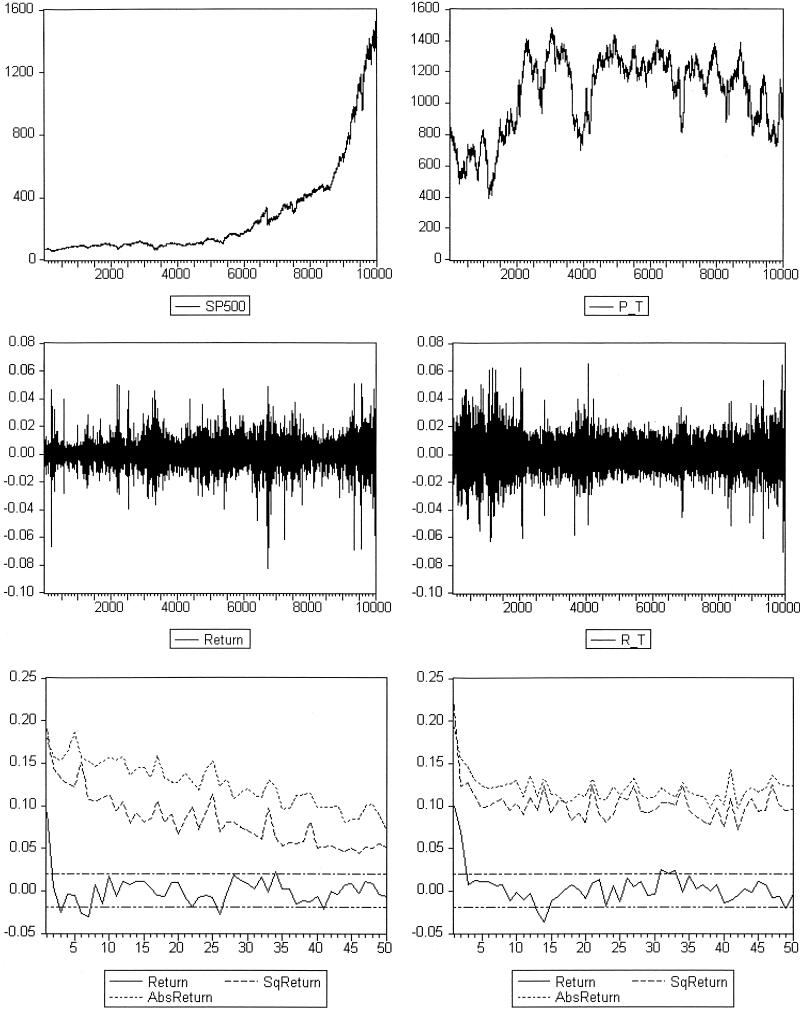
Daily S&P 500 data, 08/17/1961–05/10/2000 (Left) compared with data generated by our ABS (Right), with dynamic noise δ_t ∼ N(0, 10): price series (Top), returns series (Middle), and autocorrelation functions of returns, absolute returns, and squared returns (Bottom). Parameters are: v = 1, g = 1.9, β = 2, η = 0.99, α = 1/1,800, r = 0.001, ȳ = 1, p* = 1,000, and σ² = 1.

We next turn to the time series patterns of returns fluctuations and the phenomenon of volatility clustering. Returns are computed as relative price changes. Fig. 1 Bottom shows that the autocorrelations of the returns, squared returns, and absolute returns of the ABS-model series are similar to those of S&P 500, with (almost) no significant autocorrelations of returns and slowly decaying autocorrelations of squared and absolute returns. Returns are (linearly) unpredictable and exhibit clustered volatility. Although the ABS system considered here is a nonlinear dynamic system with only four lags, it exhibits long memory with long-range autocorrelations. Our simple stationary ABS thus exhibits a number of important stylized facts of S&P 500 returns data.

A Nonstationary Example

This section considers a simple example of a nonstationary ABS.¶ It is far from trivial to study nonlinear, nonstationary dynamical systems subject to random shocks. The example discussed below exhibits oscillatory (periodic or perhaps chaotic) fluctuations around a (stochastic) trend. There is hardly any theory about such nonlinear, nonstationary systems. For our evolutionary ABS nonstationarity makes the analysis much more complicated, because growing trends in asset prices will affect dynamic evolutionary switching of trading strategies. This section presents some preliminary simulations of nonstationary ABS.

Assume that the dividend process follows a geometric random walk—i.e.,

where ɛ_t ∼ N(0,σ_ɛ) and μ is a drift term. Beliefs on dividends are the same for all trader types and given by

A straightforward computation shows that for the dividend process (Eq. 27) the fundamental price is proportional to the dividend y_t, and thus growing at the same rate, and given by

with R = 1 + r. In our nonstationary example, beliefs about variances are given by exponentially moving averages—i.e.,

where R_t = p_t + y_t − Rp_t−1 is the excess return and 0 ≤ w ≤ 1 is a weight parameter, as in Gaunersdorfer (31).∥

In the nonstationary case, beliefs of fundamentalists are reformulated in relative terms. Fundamentalists believe that the relative deviation of the price from the fundamental value will decrease—i.e.,

or equivalently

where γ = eμ+σ/2 is the growth rate of the dividend process (and of the fundamental value). As before, technical traders believe that prices will increase (decrease) when they have increased (decreased) in the previous period—i.e.,

In the nonstationary case, the conditioning of technical trading rules on fundamentals is also modeled in relative terms, as

with ñ_2t given by the discrete choice probabilities as before.

The complete nonstationary ABS with fundamentalists versus trend extrapolators is given by:

Notice that in the nonstationary case, the model approximation error δ_t has been introduced as a random relative price change.

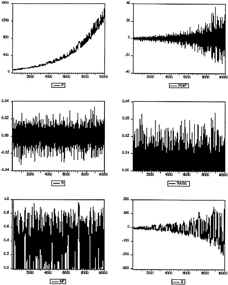
Before looking at the dynamics of the nonstationary ABS, let us have a look at the S&P 500 data again. Fig. 2 shows 10,000 time series observations of daily S&P 500 data, namely the index, changes of the index, returns (i.e., relative changes) of the index, and absolute returns. The S&P 500 index shows a strong upward trend over the past 40 years. Changes in the index increase in amplitude and exhibit clustered volatility. Relative changes or returns are unpredictable and show clustered volatility, as can also be seen from the persistence in the absolute returns series.

Fig. 2.

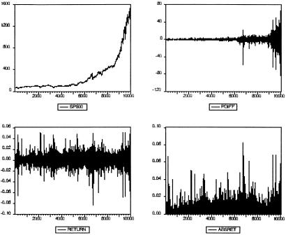
Time series for daily S&P 500 data, 08/17/1961–05/10/2000, namely the index (Top Left), changes of the index (Top Right), returns (i.e., relative changes, Bottom Left), and absolute returns (Bottom Right).

We try to reproduce these stylized facts qualitatively by the nonstationary ABS, both with and without noise. Figs. 3–6 show some typical numerical simulations, for different choices of the parameters α and g, and different levels of dividend noise σ_ɛ and model approximation noise σ_δ, with other parameters fixed at

Fig. 3 shows an example without noise, with periodic price fluctuations around a growing trend. The cycle is characterized by a large drop in prices followed by oscillatory fluctuations before a new upward price trend sets in. Price returns are periodic, with a small volatility phase with close to zero price changes interchanged with a high-volatility phase with oscillatory prices. The oscillatory phase is dominated by trend followers who cause the price to move away below the growing fundamental. As prices move too far away from the fundamental, fundamentalists start dominating the market, driving prices slowly (v = 0.99) back to the fundamental price. Although the price cycle exhibits features of volatility clustering, its pattern causes unrealistically regular and predictable asset returns.

Fig. 3.

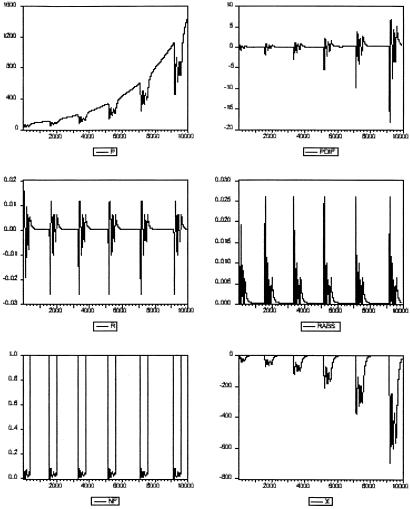
Simulated example without noise with a large-amplitude limit cycle around a growing fundamental price. Price (Top Left), price change (Top Right), return (Middle Left), absolute return (Middle Right), fraction of fundamentalists (Bottom Left), and deviation from fundamental (Bottom Right). Parameters: σ_δ = σ_ɛ = 0, α = 0.25, g = 1.03, and other parameters as in Eq. 32.

Fig. 6.

Simulated example with a noisy small-amplitude limit cycle around a growing stochastic fundamental price. Price (Top Left), price change (Top Right), return (Middle Left), absolute return (Middle Right), fraction of fundamentalists (Bottom Left), and deviation from fundamental (Bottom Right). Parameters: σ_δ = 0.005, σ_ɛ = 0.0001, α = 100, g = 1, and other parameters as in Eq. 32.

To get rid of the periodic regularity in prices and returns, we add small dividend noise (σ_δ = 0.001) and small model noise (σ_ɛ = 0.0001; i.e., 0.01%), as illustrated in Fig. 4. An immediate observation is that trend extrapolators dominate the market most of the time (see the time series of the fraction of fundamentalists), leading to deviations from the fundamental and too large fluctuations in asset prices. Returns become much more irregular, but at the same time the clustered volatility present in the noise-free limit cycle has been destroyed.

Fig. 4.

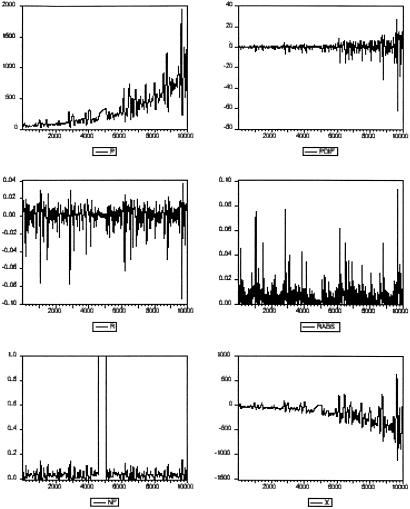
Simulated example with a large amplitude noisy limit cycle around a stochastic growing fundamental price. Price (Top Left), price change (Top Right), return (Middle Left), absolute return (Middle Right), fraction of fundamentalists (Bottom Left), and deviation from fundamental (Bottom Right). Parameters: σ_δ = 0.001, σ_ɛ = 0.0001, α = 0.25, g = 1.03, and other parameters as in Eq. 32.

Figs. 5 and 6 show a second nonstationary simulation with and without noise. In Fig. 5 a slow cycle with small amplitude around the fundamental price occurs. The smaller amplitude is due to a much larger value of α(= 100) preventing the trend extrapolators from causing large deviations from the fundamental. Small dividend noise and model noise leads to irregular fluctuations around the stochastic fundamental price, with irregular switching between fundamentalists and trend extrapolators, as illustrated in Fig. 6.

Fig. 5.

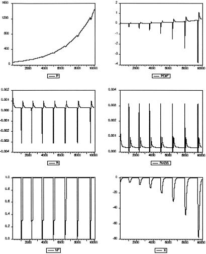
Simulated example without noise with a slow, small-amplitude limit cycle around a growing fundamental price. Price (Top Left), price change (Top Right), return (Middle Left), absolute return (Middle Right), fraction of fundamentalists (Bottom Left), and deviation from fundamental (Bottom Right). Parameters: σ_δ = σ_ɛ = 0, α = 100, g = 1, and other parameters as in Eq. 32.

Concluding Remarks

This paper has sketched simple nonlinear adaptive systems for modeling and explaining the stylized facts of financial markets. Traders switch between different forecasting strategies based on their success in the recent past. The stationary ABS, with IID dividends and a constant fundamental price, are able to match important stylized facts of financial time series, such as unpredictable returns and clustered volatility. In real markets, long price series are nonstationary, however, and it is important to take these nonstationarities into account. Some preliminary simulations of nonstationary adaptive belief systems have been presented. In the nonstationary case, the evolutionary switching of strategies interacts with nonstationarities and growing fundamental prices, which make the nonlinear, nonstationary ABS dynamics very sensitive to noise. From a qualitative viewpoint, price and return patterns in the simple nonstationary ABS seem reasonable, but more work is needed to match all autocorrelation structure in prices, returns, absolute and squared returns, and other stylized facts.

A convenient feature of our ABS is that the benchmark rational expectations model is nested as a special case. This feature gives the model flexibility with respect to experimental and empirical testing. It is worthwhile noting that Chavas (32) and Baak (33) have run empirical tests for heterogeneity in expectations in agricultural data and indeed find evidence for the presence of boundedly rational traders in the cattle market. Sharma (34) finds evidence of boundedly rational traders in financial markets. Van de Velden (35) has run asset pricing experiments and shows that, even in a stationary environment, it is hard to learn the correct, rational expectations (RE)-fundamental price level and deviations from the fundamental price are persistent. Theoretical analysis of stylized evolutionary adaptive market systems, as discussed here, and its empirical and experimental testing may contribute in providing insight into the important question of whether asset prices in real markets are driven only by news about economic fundamentals, or whether asset prices are, at least in part, driven by “market psychology.”

Abbreviations

• ABS, Adaptive Belief Systems

• EMH, Efficient Market Hypothesis

References

- 1.Kirman A. (1992) J. Econ. Perspect. 6, 117-136. [Google Scholar]
- 2.Sargent T. J., (1993) Bounded Rationality in Macroeconomics (Clarendon, Oxford).
- 3.Fama E. F. (1970) J. Finance 25, 383-423. [Google Scholar]
- 4.Shiller R. J., (1989) Market Volatility (MIT Press, Cambridge, MA).
- 5.Arthur W. B., Holland, J. H., LeBaron, B., Palmer, R. & Taylor, P. (1997) in The Economy as an Evolving Complex System II, eds. Arthur, W., Lane, D. & Durlauf, S. (Addison–Wesley, Reading, MA), pp. 15–44.
- 6.Brock W. A. (1993) Estudios Económicos 8, 3-55. [Google Scholar]
- 7.Brock W. A. (1997) in The Economy as an Evolving Complex System II, eds. Arthur, W. B., Durlauf, S. N. & Lane, D. A. (Addison–Wesley, Reading, MA), pp. 385–423.
- 8.Brock W. A. & Hommes, C. H. (1997) Econometrica 65, 1059-1095. [Google Scholar]
- 9.Brock W. A. & Hommes, C. H. (1997) in System Dynamics in Economic and Financial Models, eds. Heij, C., Schumacher, H. & Hanzon, B. (Wiley, New York), pp. 3–41.
- 10.Brock W. A. & Hommes, C. H. (1998) J. Econ. Dyn. Control 22, 1235-1274. [Google Scholar]
- 11.Chiarella C. (1992) Ann. Operations Res. 37, 101-123. [Google Scholar]
- 12.Chiarella, C. & He, T. (2002) Comp. Econ., in press.
- 13.Dacorogna M. M., Müller, U. A., Jost, C., Pictet, O. V., Olsen, R. B. & Ward, J. R. (1995) Eur. J. Finance 1, 383-403. [Google Scholar]
- 14.DeGrauwe P., DeWachter, H. & Embrechts, M., (1993) Exchange Rate Theory: Chaotic Models of Foreign Exchange Markets (Blackwell, Oxford).
- 15.De Long J. B., Shleifer, A., Summers, L. H. & Waldmann, R. J. (1990) J. Pol. Economy 98, 703-738. [Google Scholar]
- 16.Farmer, J. D. & Joshi, S. (2002) J. Econ. Behav. Org., in press.
- 17.Frankel J. A. & Froot, K. A. (1988) Greek Econ. Rev. 10, 49-102. [Google Scholar]
- 18.Hommes C. H. (2001) Quant. Finance 1, 149-167. [Google Scholar]
- 19.Kirman A. P. (1991) in Money and Financial Markets, ed. Taylor, M. (Macmillan, New York), pp. 354–368.
- 20.LeBaron B. (2000) J. Econ. Dyn. Control 24, 679-702. [Google Scholar]
- 21.LeBaron B., Arthur, W. B. & Palmer, R. (1999) J. Econ. Dyn. Control 23, 1487-1516. [Google Scholar]
- 22.Lux T. (1995) Econ. J. 105, 881-896. [Google Scholar]
- 23.Lux T. & Marchesi, M. (1999) Nature (London) 397, 498-500. [Google Scholar]
- 24.Lux, T. & Marchesi, M. (1999) Int. J. Theor. Appl. Finance, in press.
- 25.Wang J. (1994) J. Pol. Economy 102, 127-168. [Google Scholar]
- 26.Friedman M., (1953) Essays in Positive Economics (Univ. of Chicago Press, Chicago), pp. 157–203.
- 27.Manski C. & McFadden, D., (1981) Structural Analysis of Discrete Data with Econometric Applications (MIT Press, Cambridge, MA).
- 28.Anderson S., de Palma, A. & Thisse, J., (1993) Discrete Choice Theory of Product Differentiation (MIT Press, Cambridge, MA).
- 29.Gaunersdorfer A. & Hommes, C. H., (2000) A Nonlinear Structural Model for Volatility Clustering (CeNDEF working paper 00-02, University of Amsterdam).
- 30.Gaunersdorfer A., Hommes, C. H. & Wagener, F. O. J., (2000) Bifurcation Routes to Volatility Clustering (CeNDEF working paper 00-04, University of Amsterdam).
- 31.Gaunersdorfer A. (2000) J. Econ. Dyn. Control 24, 799-831. [Google Scholar]
- 32.Chavas J. P. (2000) J. Econ. Dyn. Control 24, 833-853. [Google Scholar]
- 33.Baak S. J. (1999) J. Econ. Dyn. Control 23, 1517-1543. [Google Scholar]
- 34.Sharma M., (2001) Testing for Bounded Rationality in the U.S. Financial Markets: The Case for and Against Efficient Markets (working paper, Department of Economics, University of Wisconsin).
- 35.van de Velden H., (2001) Ph.D. thesis (Department of Economics, University of Amsterdam).