Modeling civil violence: An agent-based computational approach

Abstract

This article presents an agent-based computational model of civil violence. Two variants of the civil violence model are presented. In the first a central authority seeks to suppress decentralized rebellion. In the second a central authority seeks to suppress communal violence between two warring ethnic groups.

This article presents an agent-based computational model of civil violence. For an introduction to the agent-based modeling technique, see Epstein and Axtell (1). I present two variants of the civil violence model. In the first a central authority seeks to suppress decentralized rebellion. Where I use the term “revolution,” I do so advisedly, recognizing that no political or social order is represented in the model. Perforce, neither is the overthrow of an existing order, the latter being widely seen as definitive of revolutions properly speaking. The dynamics of decentralized upheaval, rather than its political substance, is the focus here.‡ In the second model a central authority seeks to suppress communal violence between two warring ethnic groups. And, as in model I, I am interested in generating certain characteristic phenomena and core dynamics; I do not purport to reconstruct any particular case in detail, although, as discussed in Epstein et al. (6), that is an obvious long-term objective.

Civil Violence Model I: Generalized Rebellion Against Central Authority

This model involves two categories of actors. “Agents” are members of the general population and may be actively rebellious or not. “Cops” are the forces of the central authority, who seek out and arrest actively rebellious agents. Let me describe the agents first. As in all agent-based models, they are heterogeneous in a number of respects. The attributes and behavioral rules of the agents are as follows.

The Agent Specification.

First, in any model of rebellion there must be some representation of political grievance. My treatment of grievance will be extremely simple and will involve only two highly idealized components, which, for lack of better terminology, will be called hardship (H) and legitimacy (L). Their definitions are as follows:

H is the agent's perceived hardship (i.e., physical or economic privation). In the current model, this is exogenous. It is assumed to be heterogeneous across agents. Lacking further data, each individual's value is simply drawn from U(0,1), the uniform distribution on the interval (0,1). Of course, perceived hardship alone does not a revolution make. As noted in the Russian revolutionary journal, Narodnaya Volya, “No village ever revolted merely because it was hungry” [quoted in Kuran (7) and deNardo (8)]. Another crucial factor is:

L, the perceived legitimacy of the regime, or central authority. In the current model, this is exogenous and is equal across agents, and in the runs discussed below, will be varied over its arbitrarily defined range of 0 to 1.

The level of grievance any agent feels toward the regime is assumed to be based on these variables. Of the many functional relationships one might posit, we will assume:

Grievance is the product of perceived hardship (H) and perceived “illegitimacy,” if you will (1 − L).§ The intuition behind this functional form is simple. If legitimacy is high, then hardship does not induce political grievance. For example, the British government enjoyed unchallenged legitimacy (L = 1) during World War II. Hence, the extreme hardship produced by the blitz of London did not produce grievance toward the government. By the same token, if people are suffering (high H), then the revelation of government corruption (low L) may be expected to produce increased levels of grievance.

Of course, the decision to rebel depends on more than one's grievance. For example, some agents are simply more inclined to take risks than others. Accordingly, I define R as the agent's level of risk aversion. Heterogeneous across agents, this (like H) is assumed to be uniformly distributed. Each individual's level is drawn from U(0,1) and is fixed for the agent's lifetime.

All but the literally risk neutral will estimate the likelihood of arrest before actively joining a rebellion. This estimate is assumed to increase with the ratio of cops to already rebellious—so-called “active”—agents within the prospective rebel's vision. To model this, I define v as the agent's vision. This is the number of lattice positions (north, south, east, and west of the agent's current position) that the agent is able to inspect. It is exogenous and equal across agents. As in most agent-based models, vision is limited; information is local. Letting (C/A)_v denote the cop-to-active ratio within vision v, I assume the agent's estimated arrest probability P to be given by

The constant k is set to ensure a plausible estimate (of P = 0.9) when C = 1 and A = 1. Notice that A is always at least 1, because the agent always counts himself as active when computing P. He is asking, “How likely am I to be arrested if I go active?” Again, the intuition behind this functional form is very simple. Imagine being a deeply aggrieved agent considering throwing a rock through a bank window. If there are 10 cops at the bank window, you are much more likely to be arrested if you are the first to throw a rock (C/A = 10) than if you show up when there are already 29 rock-throwing agents (C/A = 1/3). For a fixed level of cops, the agent's estimated arrest probability falls the more actives there are. This simple idea will play an important role in the analysis.

Clearly, in considering whether or not to rebel, a risk-neutral agent won't care what the estimated arrest probability is, whereas a risk-averse agent will. It will therefore prove useful to define N = RP, the agent's net risk—the product of his risk aversion and estimated arrest probability. [This can be considered the special, α =0, case of N = RPJ^α, where J is the jail term, as discussed in Epstein et al. (6).] These ingredients in hand, the agent's behavioral rule is summarized in Table 1.

Table 1.

Agent state transition

State	(G − N)	State transition
Q	>T	Q⇒A
Q	≤T	Q⇒Q
A	>T	A⇒A
A	≤T	A⇒Q

If, for an agent in state Q, the difference G − N exceeds some non-negative threshold T, which could be zero, then that quiescent agent goes active. Otherwise, he stays quiescent. If, for an agent in state A, the difference exceeds T, then that active agent stays active. Otherwise, he goes quiescent. In summary, the agent's simple local rule is:

This completes the agent specification.

Bounded rationality.

It is natural to interpret this rule as stipulating that the agent take whichever binary action (active or quiescent) maximizes expected utility where, in the spirit of Kuran (7), G − N is the expected utility of publicly expressing one's private grievance, and T is the expected utility of not expressing it (i.e., of preference falsification, in Kuran's terminology). Typically, T is set at some small positive value. Notice, however, that if it takes negative values, like −G (i.e., the frustration level associated with preference falsification equals the grievance level itself), agents may find it rational to rebel knowing that they will suffer negative utility. It's simply worse to “sit and take it anymore.” Agents weigh expected costs and benefits, but they are not hyperrational. One might say [with all due respect to Olsen (10)] that individual rationality is “local” also, in the sense that the agent's expected utility calculation excludes any estimate of how his isolated act of rebellion may affect the social order. Notice, very importantly, that deterrence is local in this model and depends on the local (individually visible)—not the global—ratio of cops to actives, which is highly dynamic in this spatial model with movement.

The Cop Specification.

The cops are much simpler than prospective rebels. Their attributes are as follows:

v*, the cop vision, is the number of lattice positions (north, south, east, and west of the cop's current position) that the cop is able to inspect. It is exogenous and equal across cops. The cops' v* need not equal the agents' v, but will typically be small relative to the lattice size: cop vision is local also. The cops, like the other agents, have one simple rule of behavior:

Cops never defect to the revolution in this model.

Movement and Jail Terms.

Although the range of motion will vary depending on the numerical values selected for v and v*, the syntax of the movement rule is the same for both agents and cops:

Although the range of vision (v) is fixed, agent information (the number of cops and actives they see) is heterogeneous because of movement.

Regarding jail terms for arrested actives, these are exogenous and set by the user. Specifically, the user selects a value for the maximum jail term, J_max. Then, any arrested active is assigned a jail term drawn randomly from U(0,J_max). J_max will affect the dynamics in important ways by removing actives from circulation for various durations. However, for the present version of the model with alpha implicitly set to zero (see remark above), there is no deterrent effect of increasing the jail term. Setting alpha to a positive value would produce a deterrent effect. In addition to having no deterrent effect, it is assumed that agents leave jail exactly as aggrieved as when they entered.

Measurement.

It is important to state forthrightly that I make no pretense to measuring model variables such as perceived hardship (9) or legitimacy. The immediate question is whether this highly idealized model is sufficient to generate recognizable macroscopic revolutionary dynamics of fundamental interest. If not, then issues of measurement are moot. So, the first issue is whether the model produces interesting output. In addition to data generated by the model, run-time visualization of output is very useful. My graphical strategy is as follows.

Graphics.

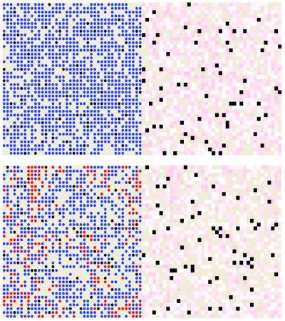
Events transpire on a lattice. Agents and cops move around this space and interact. I am interested in the dynamics of grievance and—quite separately—in the dynamics of revolutionary action. The point of separating these private and public spheres is to permit illustration of a core point in all research on this topic: public order may prevail despite tremendous private opposition to—feelings of grievance toward—a regime. Given this important distinction between private grievance and public action, two screens are shown (see Fig. 1).

Fig. 1.

Action and grievance screens.

On the right screen, agents are colored by their private level of grievance. The darker the red, the higher the level of grievance. On the left screen, agents are colored by their public action: blue if quiescent; red if active. Cops are colored black on both screens. Simply to reduce visual clutter, all agents and cops are represented as circles on the left screen and squares on the right. Unoccupied sites are sand-colored on both screens.

Runs.

To begin each run of the model, the user sets L, J, v, v*, and the initial cop and agent densities. To ensure replicability of the results, input assumptions for all runs are provided in Table 2. Agents are assigned random values for H and R, and cops and (initially) quiescent agents are situated in random positions on the lattice. The model then simply spins forward under the rule set: {A, C, M}. An agent or cop is selected at random (asynchronous activation) and, under rule M, moves to a random site within his vision, where he acts in accord with rule C (if a cop) or A (if an agent). The model simply iterates this procedure until the user quits or some stipulated state is attained. What can one generate in this extremely simple model?

Table 2.

Input assumptions for runs

	Model one				Model two
	Run 1	Run 2	Runs 3 & 4	Run 5	Run 6	Run 7	Run 8
Variable name
Cop vision	1.7	7	7	7	1.7	1.7	1.7
Agent vision	1.7	7	7	7	1.7	1.7	1.7
Legitimacy	0.89	0.82	0.9	0.8	0.9	0.8	0.8
Max. jail term	15	30	Infinite	Infinite	15	15	15
Movement	None	Random site in vision	Random site in vision	Random site in vision	Random site in vision	Random site in vision	Random site in vision
Initial cop density	0.04	0.04	0.074	0.074	0	0	0.04

All models: lattice dimensions (40×40); topology (torus); cloning probability (0.05); arrest probability constant, k (2.3); max. age (200); agent “active” threshold, for G-N (0.1); initial pop. density (0.7); agent updating (asynchronous); agent activation (once per period, random order). Departures noted in text.

Individual Deceptive Behavior.

Despite their manifest simplicity, the agents exhibit unexpected deceptive behavior: privately aggrieved agents turn blue (as if they were nonrebellious) when cops are near, but then turn red (actively rebellious) when cops move away. They are reminiscent of Mao's directive that revolutionaries should “swim like fish in the sea,” making themselves indistinguishable from the surrounding population. Ex post facto, the behavior is easily understood: the cop's departure reduces the C/A ratio within the agent's vision, reducing his estimated arrest probability, and with it his net risk, N, all of which pushes G − N over the agent's activation threshold, and he turns red. But it was not anticipated. Moreover, it would probably not have been detected without a spatial visualization (see ref. 6); individual deception would not be evident in a time series of total rebels, for example.

Free Assembly Catalyzes Rebellious Outbursts.

With both agents and cops in random motion, it may happen that high concentrations of actives arise endogenously in zones of low cop density. This can depress local C/A ratios to such low levels that even the mildly aggrieved find it rational to join. This catalytic mechanism is illustrated in Fig. 2.¶

Fig. 2.

Local outbursts.

Random spatial correlations of activists catalyze local outbursts. This is why freedom of assembly is the first casualty of repressive regimes. Relatedly, it is also the rationale for curfews. The mechanism is that local activist concentrations reduce local C/A (cop-to-active) ratios, reducing (via the equation for P above) the risk of joining the rebellion. To be the first rioter, one must be either very angry or very risk-neutral, or both. But to be the 4,000th—if the mob is already big, relative to the cops—the level of grievance and risk-taking required to join the riot is far lower. This is how, as Mao Tse Tung liked to say, “a single spark can cause a prairie fire” (quoted in ref. 7). Coincidentally, the Bolshevik newspaper founded by Lenin was called Iskra, the spark! The Russian revolution itself provides a beautiful example of the chance spatial correlation of aggrieved agents. As Kuran (7) recounts, “On February 23, the day before the uprising, many residents of Petrograd were standing in food queues, because of rumors that food was in short supply. Twenty thousand workers were in the streets after being locked out of a large industrial complex. Hundreds of off-duty soldiers were outdoors looking for distraction. And, as the day went on, multitudes of women workers left their factories early to march in celebration of Women's Day. The combined crowd quickly turned into a self-reinforcing mob. It managed to topple the Romanov dynasty within 4 days.” A random coalescence of aggrieved agents depresses the local C/A ratio, quickly emboldening all present to openly express their discontent.

A time series of total rebels is also revealing. It displays one of the hallmarks (12) of complex systems: punctuated equilibrium (Fig. 3). Long periods of relative stability are punctuated by outbursts of rebellious activity. And indeed, many major revolutions (e.g., East German) are episodic in fact.

Fig. 3.

Punctuated equilibrium.

The same qualitative pattern of behavior—punctuated equilibrium—persists indefinitely, as shown in Fig. 4, which plots the data over some 20,000 iterations of the model.

Fig. 4.

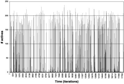
Punctuated equilibrium persists.

Waiting time distribution.

Is there any underlying regularity to these complex dynamics? For many complex systems, it turns out to be of considerable interest to study the distribution of waiting times between outbursts above some threshold. In this analysis, we set the threshold at 50 actives. An outburst begins when the number of actives exceeds 50 and ends when it falls below 50. I am interested in the time between the end of one outburst and the start of the next. Sometimes, one must wait a long time (e.g., 100 periods) until the next outburst. Sometimes, the next outburst is nearly immediate (e.g., a gap of only two periods). The frequency distribution of these inter-outburst waiting times, for 100,000 iterations of the model, is shown in Fig. 5.

Fig. 5.

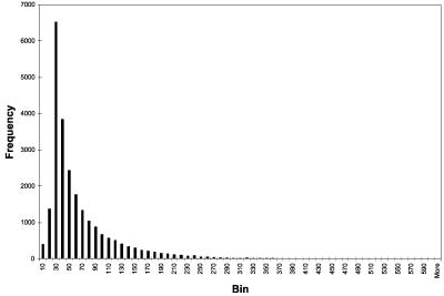
Waiting time distribution.

In the complexity literature, one often encounters the notion of an “emergent phenomenon.” I have argued elsewhere (13) that substantial confusion surrounds this term. However, if one defines emergent phenomena simply as “macroscopic regularities arising from the purely local interaction of the agents” (1), then this waiting time distribution surely qualifies. It was entirely unexpected and would have been quite hard to predict from the underlying rules of agent behavior. For instance, Fig. 5 suggests a Weibull or perhaps Lognormal distribution. Although rigorous identification is a suitable topic for future research, these data are clearly not uniformly distributed. But all distributions used in defining the agent population—the distribution of hardship and risk aversion—are uniform. In a uniform waiting time distribution, one is just as likely to wait 100 cycles as 50; that is not the case in my model, at least for these parameters. The mean of these data—the average duration between outbursts—is 60. (The SD is 55.) Clearly, most of the probability density is concentrated around this value: this means that one is much more likely to see successive outbursts within 60 cycles than within 100.

If one is willing to truncate this distribution—throwing out the most high-frequency events (waiting times less than 30 cycles), the remaining distribution is well fit by the negative exponential. In particular, the logged (truncated) data are shown in Fig. 6.

Fig. 6.

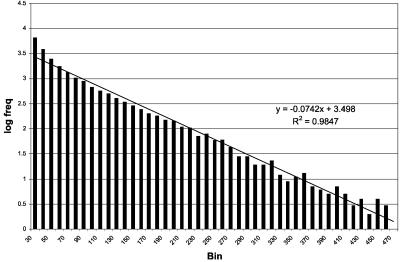
Logged data (truncated).

Ordinary least-squares regression yields an R-squared of 0.98 with slope −0.07 and intercept 3.5. The negative exponential distribution is ubiquitous in the analysis of failure rates—the rates at which electrical and mechanical systems break down. It would be interesting if “social breakdowns” followed a similar distribution. Another obvious issue is the sensitivity of this distribution to variations in key parameters. For example, how would an increase in the jail term deform the distribution? One might conjecture that, by removing rebellious agents from circulation for a longer period, increasing the jail term would “flatten” the distribution and raise its mean. All of these issues could be fruitfully explored in the future. For the moment, the core point is that a powerful statistical regularity underlies the model's punctuated equilibrium dynamics.

Outburst size distribution.

A second natural statistical topic is the size distribution of rebellious outbursts. To study this, I use the same parameterization as above and adopt the same threshold: 50 actives. But there are numerous ways to measure outburst size for statistical purposes. For example, imagine a flare-up lasting 5 days with the following number of actives per day: 60, 100, 120, 95, and 80. This outburst has a peak active level of 120. It has average (daily) activation of 100 and total activation (the sum) of 500. The size distribution of outbursts using the total activation measure is shown in Fig. 7.

Fig. 7.

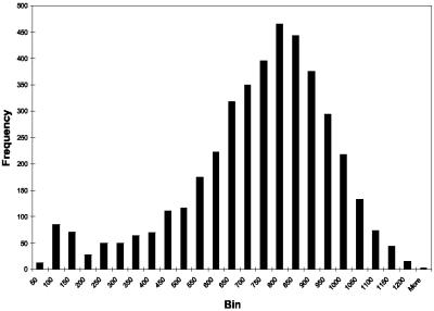
Total activation distribution.

The mean and SD are, respectively, 708 and 230. The distributions using the peak and average data are qualitatively similar. As in the case of the waiting time distribution, one could conduct further analysis to identify the best fit to Fig. 7. The point to emphasize here is not which distribution is best, but that some macroscopic regularity emerges. A strength of agent models is that they generate a wealth of data amenable to statistical treatment.

A ripeness index.

Turning to another topic, we often speak of a society as being “ripe for revolution.” In using this terminology, I have in mind a high level of tension or private frustration. Does the present model allow me to quantify this in an illuminating way? As a first cut, I noted earlier that society can be bright red on the right screen (indicating a high level of grievance) while being entirely blue on the left (indicating that no one is expressing, or “venting,” their grievance). So, if this combination of high average grievance Ḡ on the right and high frequency of blues B̄ on the left were the best indicator of high tension, a reasonable “ripeness” index would be simply their product: Ḡ B̄. This, however, ignores the crucial question, why are agents blue? If they are inactive simply because they are risk averse and have no inclination to go active, then they are not truly frustrated in the inactive blue state. So, for fixed Ḡ and B̄ a good tension index should increase as average risk aversion falls (more agents want to act out, but are nonetheless staying blue). Hence, a better simple measure is: Ḡ B̄/R̄, where R̄ is average risk aversion. In Fig. 8, I plot this against a curve of actives designed to exhibit high volatility. It is clear that a buildup of tension precedes each outburst and might be the basis of a warning indicator.

Fig. 8.

Tension (blue) and actives (red).

I turn now to a comparison of two runs involving reductions in legitimacy.∥ Both runs begin with legitimacy at a high level. In the first, I execute a large absolute reduction (from L = 0.9 to L = 0.2) in legitimacy, but in small increments (of a percent per cycle). In the second, I reduce it far less in absolute terms (from L = 0.9 to L = 0.7), but do so in one jump. Which produces the more volatile social dynamics, and why?

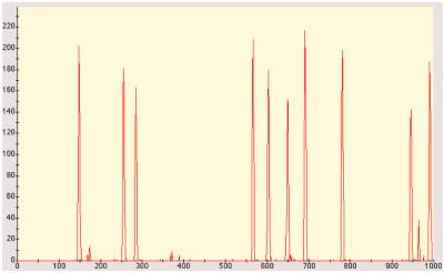
Salami Tactics of Corruption.

Fig. 9 shows the results when I reduce legitimacy in small increments. It displays three curves. The downward sloping upper curve plots the steady incremental decline in legitimacy over time. (To make these graphs clear, I actually plot 1,000 L.) The horizontal red curve just above the time axis shows the number of actives in each time period. Even though legitimacy declines to zero, there is no red spike, no explosion, because—as discussed earlier—each new active is being picked off in isolation, before he can catalyze a wider rebellion. And this is why the middle curve—representing the total jailed population—rises smoothly over time.

Fig. 9.

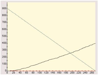
Large legitimacy reduction in small increments.

The same variables are plotted in Fig. 10. However, the scenario is different. I hold legitimacy at its initially high level (of 0.90) for 77 periods. Then, in one jump, I reduce it to 0.70, where it stays. The upper legitimacy curve is a step function. Even though the absolute legitimacy reduction (of 0.30) is far smaller than before, there is an explosion of actives, shown by the red spike. And, in turn, there is a sharp rise in the jailed population, whose absolute size exceeds that of the previous run.

Fig. 10.

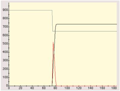
Small legitimacy reduction in one jump, t = 77.

Now, why the difference? In the incremental legitimacy reduction scenario, the potentially catalytic agents at the tail of the grievance distribution are being picked off in isolation, before they can stimulate a local contagion. The sparks, as it were, are doused before the fire can take off. In the second—one-shot reduction—case, even though the absolute legitimacy decline is far smaller, multiple highly aggrieved agents go active at once. And by the same mechanism as discussed earlier, this depresses local C/A ratios enough that less aggrieved agents jump in. Hence, the rebellious episode is greater, even though the absolute legitimacy reduction is smaller. It is the rate of change—the derivative—of legitimacy that emerges as salient.

This result would appear to have important implications for the tactics of revolutionary leadership. Rather than chip away at the regime's legitimacy over a long period with daily exposés of petty corruption, it is far more effective to be silent for long periods and accumulate one punchy exposé. Indeed, the single punch need not be as “weighty,” if you will, as the “sum” of the daily particulars. (The one-shot legitimacy reduction need not be as great as the sum of all of the incremental deltas.) Perhaps this is why Mao would regularly seclude himself in the mountains in preparation for a dramatic reappearance, and why the return of exiled revolutionary leaders—like Lenin and Khomeini—are attended with such trepidation by authorities. Perhaps this is also why dramatic “triggering events” (e.g., assassinations) loom so large in the literature on this topic; often, they are instances in which the legitimacy of the regime suddenly takes a dive. By the same token, the earlier run (incremental legitimacy reductions) explains the counterrevolutionary value of agent provocateurs: they incite the most aggrieved agents to go active prematurely, allowing them to be arrested before they can catalyze the wider rebellion.** While often sufficient, sharp legitimacy reductions are not the only inflammatory mechanism.

Cop Reductions.

Indeed, “it is not always when things are going from bad to worse that revolutions break out,” wrote de Tocqueville (14). “On the contrary, it oftener happens that when a people that has put up with an oppressive rule over a long period without protest suddenly finds the government relaxing its pressure, it takes up arms against it.” According to Kuran (7), in the cases of the French, Russian, and Iranian revolutions, “substantial numbers of people were privately opposed to the regime. At the same time, the regime appeared strong, which ensured that public opposition was, in fact, unalarming. What, then, happened to break the appearance of the invincibility of the regime and to start a revolutionary bandwagon rolling? In the cases of France and Iran, the answer seems to lie, in large measure, in a lessening of government oppression.” Indeed, de Tocqueville wrote that “liberalization is the most difficult of political arts.” Here I interpret liberalization as cop reductions. Beginning at a high level, I walk the level of cops down. Fig. 11 shows the typical result.

Fig. 11.

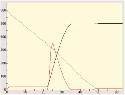
Cop reductions.

Unlike the case of incremental legitimacy reductions above (salami tactics), there comes a point at which a marginal reduction in central authority does “tip” society into rebellion. The dynamics under reductions in repressive potential (cops) are fundamentally different from the dynamics under legitimacy reduction in this model—and perhaps in societies. Because both types of reduction are emboldening to revolutionaries, one might have imagined that reductions in the regime's repressive power—the cop level—would produce dynamics equivalent to those under legitimacy reduction. As we see, however, the dynamics are fundamentally different.

Stylized Facts Generated in Model I.

Although model I is exploratory and preliminary, it does produce noteworthy phenomena with some qualitative fidelity and therefore seems, at the very least, promising. It showed, first, the unexpected emergence of individually deceptive behavior, in which privately aggrieved agents hide their feelings when cops are near, but engage in openly rebellious activity when the cops move away. In general, the model naturally represents political “tipping points”—revolutionary situations in which the screen is blue on the left (all agents quiescent) but red on the right. Surface stability prevails despite deep and widespread hostility to the regime. When pushed beyond these tipping points, the model produces endogenous outbursts of violence and punctuated equilibria characteristic of many complex systems. For some parameter settings, the size distribution of rebellious outbursts and the distribution of waiting times between outbursts exhibit remarkable regularities. The model explains standard repressive tactics like restrictions on freedom of assembly and the imposition of curfews. Such policies function to prevent the random spatial clustering of highly aggrieved risk-takers, whose activation reduces the local cop-to-active ratio, permitting other less aggrieved and more timid agents to join in. This same catalytic dynamic underlies the intriguing “salami tactic” result: Legitimacy can fall much farther incrementally than it can in one jump, without stimulating large-scale rebellion. The reason is that, in the former (salami) case, the tails of the radical distribution—the sparks—are being picked off before they can catalyze joining by the less aggrieved, and this had implications for both revolutionary and counterrevolutionary tactics. The model bears out de Tocqueville's famous adage that “liberalization is the most difficult of political arts,” showing that (quite unlike legitimacy reductions) incremental reductions in repressive potential (cops) can produce large-scale tipping events.

It should be added that the individual-level specification is quite minimal, imposing bounded demands on the agent's (and cops) information and computing capacity, while still insisting that the agent crudely weigh expected benefits against expected costs in deciding how to act. Agents are boundedly rational and locally interacting; yet interesting macroscopic phenomena emerge.

As noted at the outset, the model seems most promising for cases of decentralized upheaval. Although one could argue that certain effects of revolutionary leadership—reductions in perceived legitimacy through rousing speeches or writings that expose regime corruption—are captured, explicit leadership as such is really not modeled. That could be a weakness in cases—for example, the communist Chinese revolution—where central leadership was important, although some would argue that, even there, the main issue was not the individual leader, but society's “ripeness for revolution.” As Engels wrote, “in default of Napoleon, another would have been found” (cited in ref. 7). My tension index might be a crude measure of this ripeness.

Let me turn now to situations of interethnic violence.

Civil Violence Model II: Inter-Group Violence

Although distinct cultural groups have been generated in agent-based computational models (1, 15), here, I will posit two ethnic groups: blue and green. Agents are as in model I and turn red when active. But now, “going active” means killing an agent of the other ethnic group. The killing is not confined to agents of the out-group known to have killed. It is indiscriminant. In this variant of the model, legitimacy is interpreted to mean each group's assessment of the other's right to exist, and for the moment, L is exogenous and the same for each group. [In Epstein et al. (6), we indicate how the model might be extended to endogenize legitimacy, allowing it to vary over time, and to take different values for each group.] For model II, I also introduce some simple population dynamics. Specifically, agents clone offspring onto unoccupied neighboring sites with probability p each period. Offspring inherit the parent's ethnic identity and grievance. Because there is birth, there must be death to prevent saturation. Accordingly, agents are assigned a random death age from U(0, max_age). Here, max_age = 200. Cops are as before, and arrest—evenhandedly—red agents within their vision. (This assumption of even-handedness can, of course, be relaxed.) There is no in-group policing in this version of the model, although Fearon and Laitin (16) argue convincingly that this may be important in many cases.

Peaceful Coexistence.

For the first run of model II, I set legitimacy to a high number, just to check whether peaceful coexistence prevails with no cops. Fig. 12 depicts a typical situation.

Fig. 12.

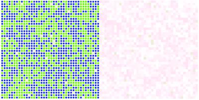
Peaceful coexistence.

The left screen clearly shows spatial heterogeneity and peaceful mixing of groups with no red agents. On the right, only the palest of pink shades, indicating low levels of grievance, are seen. Harmonious diversity prevails. However, with no cops to regulate the competition, if L falls, even to 0.8, the picture darkens substantially. Indeed, ethnic cleansing results.

Ethnic Cleansing.

The sequence of five panels in Fig. 13 clearly shows local episodes of ethnic cleansing, leading ultimately to the annihilation of one group by the other: genocide.

Fig. 13.

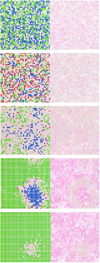
Local ethnic cleansing to genocide.

Over a large number of runs (n = 30), genocide is always observed. The victor is random. The phenomenon is strongly reminiscent of “competitive exclusion” in population biology (see ref. 17). When two closely related species compete in a confined space for the same resource, one will gain an edge and wipe the other out. If, however, the inter-species competition is regulated by a predator that feeds evenhandedly on the competitors, then both can survive. Peacekeepers are analogous to such predators. I introduce them presently.

Safe Havens.

I begin this run exactly as in the previous genocide case. But, at t = 50, I deploy a force of peacekeepers. They go to random unoccupied sites on the lattice. And this typically produces safe havens. A representative result is shown in Fig. 14.

Fig. 14.

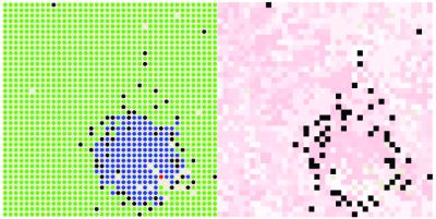
Safe havens emerge under peacekeeping.

Rather than begin with no cops initially, as in the previous run, a case with high initial cop density was also examined. Once a stable pattern had emerged, the cops were withdrawn. Here, with heavy authority from the start (a high cop density of 0.04), a stable, but nasty, regime emerges. The presence of cops prevents either side from wiping the other out, but their coexistence is not peaceful: ethnic hostility is widespread at all times. When (ceteris paribus) all cops are withdrawn—the peacekeepers suddenly go home—there is reversion to competitive exclusion and, eventually, one side wipes out the other.

Clearly, peacekeeping forces can avert genocide. But what is the overall relationship between the size of a peacekeeping presence and the incidence of genocide? As an initial exploration of this complex matter, a sensitivity analysis on cop density is conducted.

Cop Density and Extinction Times.

For purposes of this analysis, all cops are in place at time 0. But there will be random run-to-run variations in their initial positions and, of course, in their subsequent movements. These initial cop densities are systematically varied from 0.0 up to 0.1, in increments of 0.002. For each such value, the model was run 50 times until the monochrome—genocide—state was reached. (If it was not reached after 15,000 cycles, the run was terminated.) The data appear in Fig. 15.

Fig. 15.

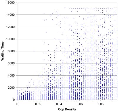
Waiting time and initial cop density data.

There are three things to notice. First, at low force densities (0 to 0.02), convergence to genocide is rapid. Second, the same rapid convergence to genocide is observed at all force densities. Third, reading vertically, at high force densities (0.08 and above), there is high variance. One can have high effectiveness (delays of over 15,000 cycles) or extremely low effectiveness (convergence in tens of cycles). The devil would appear to be in the details in peacekeeping operations.

As noted earlier, the model was run 50 times at each density (with a different random seed each time). So, at each density, there is a sample distribution of waiting times over the 50 runs. I plot the means of these distributions at each initial density in Fig. 16, along with the best linear fit to the same data.

Fig. 16.

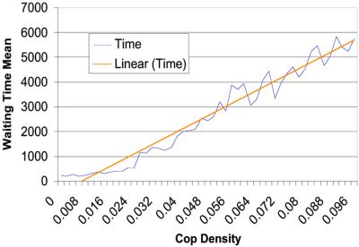
Waiting time mean and initial cop density.

On average, the larger the initial force of peacekeepers, the more time one buys. At the same time, however, the SD is also rising, as shown in Fig. 17. Hence, the confidence interval about the mean is expanding. Thus, as the mean waiting time to genocide grows, we have decreasing confidence in it as a point estimate of the outcome, all of which is to say, perhaps, that the peacekeeping process is highly path dependent and uncertain. (Giving cops the capacity to communicate could affect these results.)

Fig. 17.

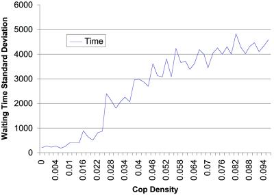
Waiting time standard deviation and initial cop density.

This entire analysis proceeds from the assumption that all forces are in place at time 0. The same analysis could be conducted for different arrival schedules. At the moment, the claim is simply that the agent-based methodology permits one to study the effects of early and late interventions of different scales, which is obviously crucial in deciding how to size, design, and operate peacekeeping forces.

Summary Of Model II Results.

With high legitimacy (mutual perception by each ethnic group of the other's right to exist), peaceful coexistence between ethnic groups is observed; no peacekeepers are needed. However, if the force density is held at zero, and legitimacy is reduced (to 0.8), local episodes of ethnic cleansing are seen, leading to surrounded enclaves of victims, and ultimately to the annihilation of one group by the other. With early intervention on a sufficient scale, this process can be stopped. Safe havens emerge. With high cop density from the outset, the same level of legitimacy (0.8) produces a stable society plagued by endemic ethnic violence. If cops are suddenly removed, there is reversion to competitive exclusion and genocide. The statistical relationship between initial cop densities and the waiting time to genocide was studied. Although the mean relationship was positive, quick convergence to genocide at extremely high force levels, it was shown, is not precluded, because of the path-dependent and highly variable dynamics of interethnic civil violence.

Conclusion

Agent-based methods offer a novel and, I believe, promising approach to understanding the complex dynamics of decentralized rebellion and interethnic civil violence, and, in turn, to fashioning more effective and efficient policies to anticipate and deal with them.††

References

- 1.Epstein J. M. & Axtell, A., (1996) Growing Artificial Societies: Social Science from the Bottom Up (MIT Press, Cambridge, MA).
- 2.Collier P. (2000) J. Conflict Resolution 44, 839-850. [Google Scholar]
- 3.Collier P. & Hoeffler, A. (1998) Oxford Econ. Papers 50, 563-573. [Google Scholar]
- 4.Collier P. & Hoeffler, A., (1999) Justice-Seeking and Loot-Seeking in Civil War, Working Paper, April (World Bank, Washington, DC).
- 5.Collier P. & Hoeffler, A., (2001) Greed and Grievance in Civil War, Policy Research Working Paper 2355 (World Bank, Washington, DC).
- 6.Epstein J. M., Steinbruner, J. D. & Parker, M. T., (2001) Modeling Civil Violence: An Agent-Based Computational Approach, Working Paper 20 (Center on Social and Economic Dynamics, Washington, DC).
- 7.Kuran T. (1989) Public Choice 61, 41-74. [Google Scholar]
- 8.DeNardo J., (1985) Power in Numbers: The Political Strategy of Protest and Rebellion (Princeton Univ. Press, Princeton).
- 9.Graham C. & Pettinato, S., (2002) Happiness and Hardship: Opportunity and Insecurity in New Market Economies (Brookings Institution Press; Washington, DC).
- 10.Olson M., (1971 1965) The Logic of Collective Action: Public Goods and the Theory of Groups (Harvard Univ. Press, Cambridge, MA).
- 11.Epstein J., (2003) Generative Social Science: Studies in Agent-Based Computational Modeling (Princeton Univ. Press, Princeton), in press.
- 12.Young H. P., (1998) Individual Strategy and Social Structure (Princeton Univ. Press, Princeton).
- 13.Epstein J. (1999) Complexity 4/5, 41-60. [Google Scholar]
- 14.de Tocqueville A., (1955 1856) The Old Regime and the French Revolution, trans. Gilbert, S. (Doubleday, New York).
- 15.Axelrod R. (1997) J. Conflict Resolution 41, 203-226. [Google Scholar]
- 16.Fearon J. D. & Laitin, D. D. (1996) Am. Polit. Sci. Rev. 90, 715-735. [Google Scholar]
- 17.May R. M., (1981) Theoretical Ecology: Principles and Applications (Blackwell, Oxford).
- 18.Dean J. S., Gumerman, G. J., Epstein, J. M., Axtell, R. L., Swedlund, A. C., Parker, M. T. & McCarroll, S. (2000) in Dynamics in Human and Primate Societies: Agent-Based Modeling of Social and Spatial Processes, eds. Kohler, T. A. & Gumerman, G. J. (Oxford Univ. Press, New York), pp. 187–214.