Bias and Efficiency in Family-Based Gene-Characterization Studies: Conditional, Prospective, Retrospective, and Joint Likelihoods

Abstract

We revisit the usual conditional likelihood for stratum-matched case-control studies and consider three alternatives that may be more appropriate for family-based gene-characterization studies: First, the prospective likelihood, that is, Pr(D|G,𝒜); second, the retrospective likelihood, Pr(G|D); and third, the ascertainment-corrected joint likelihood, Pr(D,G|𝒜). These likelihoods provide unbiased estimators of genetic relative risk parameters, as well as population allele frequencies and baseline risks. The parameter estimates based on the retrospective likelihood remain unbiased even when the ascertainment scheme cannot be modeled, as long as ascertainment only depends on families’ phenotypes. Despite the need to estimate additional parameters, the prospective, retrospective, and joint likelihoods can lead to considerable gains in efficiency, relative to the conditional likelihood, when estimating genetic relative risk. This is true if baseline risks and allele frequencies can be assumed to be homogeneous. In the presence of heterogeneity, however, the parameter estimates assuming homogeneity can be seriously biased. We discuss the extent of this problem and present a mixed models approach for providing consistent parameter estimates when baseline risks and allele frequencies are heterogeneous. The efficiency gains of the mixed-model prospective, retrospective, and joint likelihoods relative to the efficiency of conditional likelihood are small in the situations presented here.

Introduction

Segregation and linkage analyses can give us some information on the penetrance of different genotypes. However, since they do not involve measuring the putative causal gene(s), they can be very inefficient (Gauderman and Faucett 1997). In the future, as candidate genes become quicker and cheaper to identify and measure, gene-characterization studies will play an important role in measuring parameters such as penetrance.

Gene-characterization studies involve measuring the properties of a given, observable gene as it relates to a disease (or diseases) of interest. Typically, this means parameters measuring the penetrance of different genotypes and allele frequencies. Since it is possible—although expensive and logistically difficult—to observe the genotypes of all subjects in a study, gene-characterization studies have much in common with traditional epidemiological studies which measure the association of a disease with an observable covariate. Still, there are problems and opportunities particular to gene-characterization studies.

The diseases of interest in gene-characterization studies are usually rare, as are the putative high-risk alleles. This means traditional population-based case-control and cohort studies are inefficient, since most subjects will not have the exposure of interest. Some of the strategies to deal with this problem involve only sampling families with at least one case, or sampling heavily affected families in an ad hoc manner. The analysis of such data requires a correction for the sampling method, or ascertainment.

Gene-characterization studies are also susceptible to genetic confounding. Population controls are subject to “population-stratification bias,” where allele frequencies and penetrances vary between subpopulations which are impossible to match on (Lander and Schork 1994; Witte et al. 1999). Sibling controls are immune to population stratification bias when analyzed using a standard stratum-matched conditional likelihood, but they may be less efficient than population controls (Witte et al. 1999).

The methods presented in this paper take advantage of our ability to model the dependence of genotypes within families when analyzing gene-characterization studies. This can increase efficiency by making more effective use of subjects on whom we have both trait and genotype data and by use of subjects on whom we only have trait data. As in segregation analysis, even subjects who are not genotyped can contribute information about the relationship between the trait and the gene being studied.

The study of breast cancer throughout the last decade provides an example of the development from linkage and segregation studies to gene-characterization studies. Before BRCA1 had been cloned, investigators could only use segregation and linkage analyses to estimate penetrance in carriers of BRCA1 (e.g., Claus et al. 1991; Easton et al. 1993, 1995). Once BRCA1 had been cloned, investigators could use the actual, observed genotypes of individuals in their analyses. For example, Struewing et al. (1997) genotyped volunteers, regardless of their disease status, and then compared the disease status of relatives of carriers and noncarriers. Their analysis did not actually make use of the medical history of the genotyped volunteers. Gail et al. (1999) extended this design to accommodate stratified sampling based on the disease status of the probands and additional genotype data on other relatives.

In this study, we examine the properties of several methods of analyzing case-control data on sibships. The design we consider differs from those in Struewing et al. (1997) and Gail et al. (1999) in that it uses disease status data on all subjects (where available) and restricts sampled sibships to those with at least one case and one control. These methods can be extended to larger pedigrees (Siegmund et al. 1999), but, for simplicity, we restrict our attention to sibship-based designs. We assume complete ascertainment, an assumption which would hold if, for example, investigators were sampling sibships with at least one case and one control at random from a larger ongoing cohort study (Elston and Bonney 1984). We also assume that the outcome of interest is binary (present / absent). Age-at-onset models are, of course, relevant for diseases such as cancer, but are beyond the scope of this paper. We sketch extensions of the likelihoods developed here which incorporate age-at-onset models in the discussion.

In the first section, we present four likelihoods for the analysis of case-control data on sibships: the conditional, prospective, retrospective, and joint likelihoods. The conditional likelihood is the usual likelihood for stratum-matched data; the prospective likelihood is based on modeling the risk of disease given genotypes; the retrospective likelihood is based on modeling the distribution of genotypes given the phenotypes (disease); and the joint likelihood is based on the joint probability of genotypes and phenotypes.

The conditional and retrospective likelihoods are “ascertainment-assumption free”—that is, if the probability of a family being ascertained depends only on the family members’ phenotypes, then we do not have to explicitly model how ascertainment depends on phenotypes. Because of this property, the retrospective likelihood can easily and correctly analyze designs which restrict ascertainment to sibships with multiple cases or to sibships with affected parents. The hope is that such designs will increase efficiency, because multiple-case families are more likely to carry the disease gene. The retrospective likelihood is related to the “MOD score” approach in linkage analysis, which has been widely used because of its ability to correct for ascertainment in an “assumption-free” manner (Easton et al. 1993; Easton et al. 1995; Hodge and Elston 1994). We put quotes around “assumption-free,” because it is important to remember that the retrospective likelihood only corrects for ascertainment if ascertainment does not depend directly on genotypes or other covariates included in the model (Siegmund et al. 1999). We return to this restriction in the discussion.

In the second section, we examine the relative efficiencies of conditional, prospective, retrospective, and joint logistic likelihoods. In the third section, we examine the bias that results in the prospective, retrospective, and joint likelihoods when there is heterogeneity in baseline familial disease rates and allele frequencies. In the fourth section, we present a mixed-model approach which allows for unbiased parameter estimation, even in the case of heterogeneity. We summarize and compare the properties of the four likelihoods in the Discussion section.

Likelihoods for Sibship-Based Case-Control Studies

Each of the four likelihoods presented below is, in some sense, a conditional likelihood, since for each the contribution for a single family can be written as

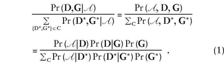Here D denotes the vector of phenotype information for the family members, G is the vector of measured genes, 𝒜 is the event that the family was ascertained, and the sum in the denominator is over all events in some conditioning set C (G^* etc. are dummy variables, whereas D and G are observed). For example, in the case of what we call the retrospective likelihood, C consists of all combinations {D^*,G^*} with D^* equal to the observed phenotypes. In other words, the sum in the denominator is over all possible genotypes while holding D fixed. Throughout the rest of this paper when we say “conditional likelihood,” we are only referring to the usual conditional likelihood for stratum-matched data, presented immediately below.

A basic principle of case-control methodology is that subject selection should directly depend only upon potential subjects’ disease status, not on their covariates. This is why the term Pr(𝒜|D,G) simplifies to Pr(𝒜|D) in the above likelihood. In this paper we assume complete ascertainment, where Pr(𝒜|D)=1 if D is in the ascertainment set (e.g., it has one case and one control), and 0 otherwise. Complete ascertainment is often assumed, as a mathematical convenience, in situations where it is difficult to verify, but again it is worth noting that we can actually achieve complete ascertainment if we are randomly sampling families who meet entry requirements from an ongoing population-based cohort study. The conditional and retrospective likelihoods can accommodate other ascertainment schemes which only depend upon subjects’ phenotypes without modification; the prospective and joint likelihoods require that the model for ascertainment be changed appropriately.

As in most epidemiologic studies, we further assume that subjects’ phenotypes are conditionally independent, given their covariates, so that Pr(D|G)=iPr(D_i|G_i). In particular, this means we assume that the candidate gene is not in linkage disequilibrium with another gene related to disease. In a subsequent section, we consider violations of the assumption of conditional independence—most notably, population stratification.

Throughout this study, we assume a simple main-effect logistic model for the candidate gene. That is, . Here Z(G) is a coding of the genotype depending upon dominance assumptions. For example, in the calculations we describe below, we assumed a two-allele model: Z(aa)=0, Z(Aa)=δ, Z(AA)=1, where δ=0, 1/2, 1 for recessive, additive, and dominant models, respectively. There are other models for Pr(D|G), such as the log-linear model , and these could be used in (1) as well. We use the logistic model because it is the most common and does not require constraints on the parameters to ensure Pr(D|G)⩽1.

Main effects for measured environmental factors and gene-environment interactions can be added to the conditional and prospective likelihoods without further assumptions. They can be added to the other two likelihoods as long as the genetic and environmental factors are independent, that is, if Pr(G|Z_env)=Pr(G).

The term Pr(G) in (1) is parameterized by q, the mutant allele frequency. We will denote the penetrance in carriers as and the penetrance in noncarriers as .

Although, for simplicity, we mainly consider sibship studies in this paper, these likelihoods can be extended to include nuclear families and larger pedigrees. They can also accommodate designs where some of the subjects are not genotyped. For example, in a study of nuclear families we may not be able to genotype the parents. Then, the joint probability of the observed phenotypes and genotypes for a family simply becomes a sum over unknown parental genotypes (Siegmund et al. 1999).

In this section and the next we assume that the baseline rate and allele frequency are homogeneous, that is, α and q do not vary between or within families. We consider the case where these parameters are allowed to vary between families in a subsequent section.

Conditional Likelihood

The usual conditional likelihood for matched case-control studies conditions on the number of observed cases in each matched set (family). The likelihood contribution for a given family takes the following form:

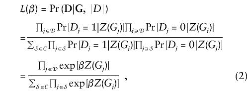where 𝒟 denotes the set of cases and 𝒞 denotes the set of subsets of family members of size . The conditional likelihood does not depend upon the baseline risk parameters and hence is valid even if the baseline differs between (but not within) families. If cases and controls are matched on age or other factors, the standard conditional likelihood requires no assumptions about the dependence of the baseline risk on these factors. Note that without relying on auxiliary information from population rates, the standard conditional likelihood cannot estimate absolute penetrance, only the genetic odds ratio, exp(β).

As Breslow and Day (1980, p. 248) note, the conditional likelihood is both prospective and retrospective.

[P]recisely the same (conditional) likelihood is obtained whether we regard the data as arising from either (i) a prospective study of n individuals with a given set of exposures…, the conditioning event being the observed number n₁ of cases arising in the sample; or (ii) a case-control study involving n₁ cases and n₀ controls, the conditioning event being the n observed exposure histories.

That is,

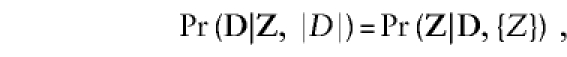where Z is the vector of observed exposures and {Z} is the set of observed exposures. Because the conditioning event on the right includes D, this likelihood corrects for ascertainment in an “ascertainment assumption free” manner just as the retrospective likelihood does (see below). The retrospective likelihood differs from the conditional likelihood in that it does not condition on the set of observed exposures (genotypes).

Prospective Likelihood

Suppose that, in sibships of size 2, the ascertainment rule 𝒜 were that there be exactly one case and one control. Then the ascertainment event 𝒜 is {d₁+d₂=1}, which is identical to the conditioning event for the conditional likelihood. However, for larger sibships, one might consider a requirement that there be at least one case and one control. The standard conditional likelihood, equation (2) would then condition on the observed number of cases, which is a stronger requirement than necessary. One could, instead, consider what we shall call the prospective likelihood of the form ℒ(α,β)=Pr(𝒜|D)Pr(D|Z)/Pr(𝒜|Z) where 𝒜 now includes all D vectors that would qualify for ascertainment. For example, in sibships of size 3, there are six possible events that would qualify for ascertainment in such a case-control study, D=(1,0,0)^′, (0, 1, 0)′, (0, 0, 1)′, (1, 1, 0)′, (1, 0, 1)′, or (0, 1, 1)′. Either the first three or the second three would be used in the conditional likelihood, depending upon whether one or two cases were observed, whereas all six would be used in the full prospective likelihood. This should lead to a more efficient estimator of β. On the other hand, the additional terms include entries that have a different number of cases and controls from the numerator of the likelihood, so that the baseline risk parameter α no longer cancels out. It must therefore be estimated along with β, which could lead to some loss of efficiency. We provide some comparisons of the two likelihoods below.

Retrospective Likelihood

Prentice and Pyke (1979) introduced an alternative retrospective likelihood based on Pr(Z|D). They showed that this likelihood can be factored into two components, this first identical to the standard prospective likelihood, and the second depending upon the distribution of covariates. The maximization of the first component led to the MLE of the entire likelihood, subject to a constraint based on the marginal population disease rate (integrating over the population distribution of covariates). This approach is necessitated by the difficulty of describing the population distribution of covariates in most epidemiologic applications. However, in the genetics context, there is a strong basis for modeling the joint distribution of genotypes within families, so it becomes feasible to maximize the retrospective likelihood directly. The advantage of this approach is that by conditioning on the disease outcomes, one automatically conditions on ascertainment, thereby making this approach relevant to case-control analyses conducted within heavily loaded families for whom ascertainment correction with the usual prospective likelihood would be impossible. The disadvantage is, of course, that by conditioning on all the phenotypes, rather than just the ascertainment event, one may “overcondition,” thereby perhaps leading to some loss of efficiency relative to the analysis that would be possible if the ascertainment event could be defined. In the numerical results which follow, we show that this generally does not occur when the parameter of interest is the genetic odds ratio. However, the retrospective likelihood turns out not to be particularly efficient in estimating absolute penetrances.

A sibship’s contribution to the retrospective likelihood looks like this:

The sum in the denominator is over all possible genotype vectors for the sibship. The function p_q(G), which is the probability of observing the genotypes G, can be calculated by summing over (presumably) unknown parental genotypes, G_p,

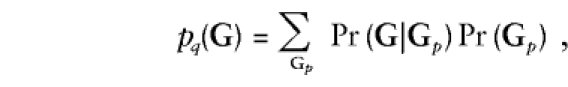where the first term is a simple Mendelian transmission probability, while the second term assumes Hardy-Weinberg equilibrium and depends on the population allele frequency q. Thus, the retrospective likelihood is a function of α, β, and the allele frequency q. As with α, we assume for this section and the next that q is constant across families and investigate the effect of heterogeneity in later sections.

The retrospective likelihood implicitly corrects for ascertainment in this case. The explicitly ascertainment-corrected retrospective likelihood, Pr(G|D,𝒜), reduces to

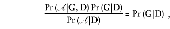because 𝒜 is assumed to be independent of G.

Note that, under this likelihood, sib-matched case-control pairs can contribute information about α. This may seem somewhat counterintuitive. Indeed, in the limit of a rare disease (more precisely, that the penetrances for all genotypes are small), the likelihood contribution for a given case-control pair simplifies to

which no longer depends upon α. When the disease is not rare, however, the terms of the form 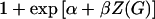from the denominator of the logistic penetrance function do not cancel out of the likelihood.

We show below that the retrospective likelihood can be significantly more efficient than the standard conditional likelihood in estimating the log genetic odds ratio β. An intuitive explanation for the greater efficiency of the retrospective likelihood is that because it does not condition on the observed genotypes, it actually conditions on less than the standard conditional likelihood—even though the latter conditions on and not D itself. This means that all case-control sets, including those that are genotype concordant, are informative.

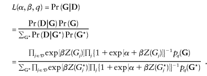
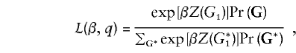
Joint Likelihood

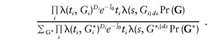
Finally, we consider the ascertainment-corrected joint likelihood

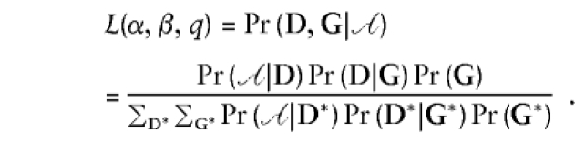Here, the sum in the denominator is over all possible genotypes and all phenotype vectors with at least one case and one control. Like the prospective and retrospective likelihoods, the joint likelihood is a function of all three parameters, but entails the weakest conditioning of all, Pr(𝒜), rather than Pr(𝒜|G) (for the prospective likelihood) or Pr(D) for the retrospective likelihood, and thus should be more efficient than either.

Efficiency Comparisons

The asymptotic efficiency of one likelihood (call it ℒ₁) relative to another (ℒ₀) for measuring a parameter θ is given by the ratio of the inverse asymptotic estimates for the variance of :

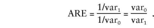The asymptotic relative efficiency (ARE) can be interpreted as the ratio of the sample sizes needed for two likelihoods to yield confidence intervals for θ with the same size. We computed the asymptotic variances for the different likelihoods by calculating the inverse of the expected information at the true parameters. The population disease rate was fixed at 10%, and the allele frequencies were chosen so as to fix the proportion of cases attributable to the at-risk genotype.

Table 1 presents the efficiencies of the prospective, retrospective, and joint likelihoods relative to the conditional likelihood for estimating the log genetic odds ratio. The prospective, retrospective, and joint likelihoods are always more efficient than (or as efficient as) the standard conditional likelihood for estimating the genetic odds ratio. The joint likelihood is always the most efficient. When the disease gene is dominant and the genetic odds ratio is large, sibships of size three and four are more than three times as efficient when analyzed by the new likelihoods. The efficiency gains over the conditional likelihood are generally smaller when the disease gene is not dominant, when the genetic odds ratio is smaller or when the sibship size decreases.

Table 1.

Asymptotic Efficiency of the Prospective, Retrospective, and Joint Likelihoods for Estimation of the Log Genetic Odds Ratio, Relative to the Conditional Likelihood^[Note]

	var0/vara
	Genetic Odds Ratio = 20			Genetic Odds Ratio = 2
	Sibship Size			Sibship Size
Model and Likelihood	2	3	4	2	3	4
	q = .14			q = .44
Recessive model:
Prospective	1.00	2.11	2.32	1.00	1.18	1.26
Retrospective	2.68	2.66	2.53	1.08	1.23	1.29
Joint	2.68	2.74	2.64	1.08	1.50	1.48
	q = .02			q = .19
Additive model:
Prospective	1.00	1.64	1.94	1.00	1.22	1.30
Retrospective	1.07	1.71	1.95	1.01	1.23	1.22
Joint	1.07	1.72	1.99	1.01	1.27	1.36
	q = .01			q = .10
Dominant model:
Prospective	1.00	3.03	3.56	1.00	1.24	1.34
Retrospective	1.13	3.17	3.28	1.05	1.27	1.37
Joint	1.13	3.47	3.74	1.05	1.37	1.45

Note.—The population disease rate was fixed at 10%, and allele frequencies were chosen so as to fix the proportion of cases caused by the genetic factor.

^avar = the asymptotic variance of the maximum-likelihood estimate for the log genetic odds ratio for the prospective, retrospective, or joint likelihood. var₀ = the asymptotic variance of the maximum-likelihood estimate for log genetic odds ratio for the standard conditional likelihood.

All other things being fixed, the qualitative relationship between the efficiencies of the four likelihoods follows the intuition that the less we condition on, the more efficient a likelihood will be. The event which the conditional likelihood conditions on contains the conditioning events for the retrospective, prospective, and joint likelihoods—hence, the conditional likelihood is the least efficient. The event which the joint likelihood conditions on is contained by the conditioning events for the other likelihoods—hence, the joint likelihood is the most efficient. The conditioning events for the prospective and retrospective likelihoods overlap but are not nested. In some conditions, the prospective is more efficient; in others, the retrospective is more efficient. The size of the efficiency differences depends on the genetic odds ratio, the mode of inheritance, sibship size, baseline rates, and allele frequencies in a complex manner.

Table 2 presents the efficiencies of the prospective and retrospective likelihoods for estimating absolute penetrance in carriers relative to the joint likelihood (recall that the conditional likelihood cannot estimate absolute penetrances). The retrospective likelihood was considerably less efficient than the prospective and joint likelihoods for estimating the penetrance in carriers (because it is highly inefficient in estimating penetrance in noncarriers and the correlation between and is large). This is consistent with the findings of Liang et al. (1996) on the inefficiency of MOD score analysis relative to a full (joint) likelihood when estimating absolute penetrances using linked markers instead of measured genotypes.

Table 2.

Efficiency of the Prospective and Retrospective for Estimating the Absolute Penetrance in Carriers, Relative to the Joint Likelihood^[Note]

	var0/vara
	Genetic Odds Ratio = 20			Genetic Odds Ratio = 2
	Sibship Size			Sibship Size
Model and Likelihood	2	3	4	2	3	4
	q = .14			q = .44
Recessive model:
Prospective	NAb	.83	.91	NAb	.95	.96
Retrospective	1.00	.51	.49	1.00	.016	.016
	q = .02			q = .19
Additive model:
Prospective	NAb	.96	.98	NAb	.99	.98
Retrospective	1.00	.11	.12	1.00	.003	.003
	q = .01			q = .10
Dominant model:
Prospective	NAb	.90	.97	NAb	.98	.98
Retrospective	1.00	.24	.22	1.00	.010	.010

Note.—The population disease rate was fixed at 10%, and allele frequencies were chosen so as to fix the proportion of cases caused by the genetic factor.

^avar = the asymptotic variance of the maximum-likelihood estimate for the log genetic odds ratio for the prospective, retrospective, or joint likelihood. var₀ = the asymptotic variance of the maximum-likelihood estimate for log genetic odds ratio for the standard conditional likelihood.

^bFor sibships of size two, the prospective likelihood is identical to the standard conditional likelihood, and hence cannot estimate absolute penetrances.

In the case of a rare disease allele, the sample sizes needed to obtain reasonable resolution for estimating penetrance with case-control sib pairs can be prohibitive. For example, for a dominant allele with frequency .0033 and true penetrances .92 and .10 in carriers and noncarriers, respectively, the retrospective and joint likelihoods require over 15,000 case-control pairs to estimate the penetrance in carriers roughly ±.10 with 95% confidence (not shown). However, these sample-size requirements decrease dramatically for sibships of size three; only 341 such sibships are needed for the joint likelihood to give the same resolution, whereas 896 are needed for the retrospective likelihood. This drop reflects the fact that case-control pairs contain very little information on allele-frequency and baseline-odds parameters; sib trios evidently have considerably more. The sample sizes needed to ensure that the estimated odds ratio is >20 with 95% probability in this case are also much smaller; about 1,200 sibships of size two for all three likelihoods are needed, and between 100 and 130 sibships of size three.

Multiple-Case Families

As mentioned in the introduction, restricting sampled families to those with multiple cases can increase efficiency for estimating the genetic odds ratio, since those families are more likely to carry the disease gene. Consider a design where we require each sibship to have at least two cases and at least one control. Under the assumptions that the population rate is 10%, the genetic odds ratio is 20, and the allele frequency is 1%, then, under this design, a sibship of size four, analyzed with the conditional likelihood, can be 3.5 times more efficient for estimating the odds ratio than can a sibship of size four under the restriction of at least one case and one control. Under the same parameter assumptions, but using the retrospective likelihood, sibships of size four with at least two cases are about 2.2 times as efficient as sibships of the same size with at least one case. The retrospective likelihood is still 3.0 times more efficient than the conditional likelihood under this more restrictive design. Another design which leads to greater efficiency gains is requiring that sampled sibships’ parents be affected.

While these multiple-case designs may increase the efficiency for estimating the genetic odds ratio, they may decrease the efficiency for estimating baseline odds and allele frequencies, thus making it more difficult to estimate absolute penetrance. They may also be more susceptible to population stratification bias. We are currently studying these designs and their analysis and will discuss their potential advantages and disadvantages in more detail in a later paper.

Bias in the Case of Heterogeneity in Baseline Risks and Allele Frequencies

The likelihoods and calculations presented in the previous two sections assumed that the baseline risks and allele frequencies were homogeneous. Two kinds of residual familiality could violate this assumption. First, there may be dependencies in disease risks between family members caused by shared unmeasured risk factors (either genetic or environmental). Such dependencies could be complex, but, in the absence of specific knowledge of their source, one might simply consider each family to be a homogeneous unit with the same, unknown baseline risk parameter. Second, families may derive from a heterogeneous population with strata that have different allele frequencies. Neither of these types of heterogeneity poses any problem for the conditional likelihood, because all comparisons are made within families and the likelihood is not a function of either baseline risks or population allele frequencies. However, they pose a greater problem for the prospective, retrospective, and joint likelihoods.

We assume that the genetic effect itself (i.e., β) is constant. If β varies between families, then estimates based on a homogeneous β will estimate some form of weighted average of the family-specific βs. We do not consider this situation further here, on the grounds that if there is really heterogeneity in β, then we really need to measure its distribution and not just an average or median β. Similarly, we do not consider estimations of penetrance in this section or the next, because if there is heterogeneity in baseline odds ratios, then there will necessarily be heterogeneity in penetrance. Our main interest in these sections is estimating the log odds ratio, β.

The retrospective likelihood is a function of α only when the denominator of the logistic function is substantially different from 1. Thus, it follows that the first type of heterogeneity can be ignored for “rare” diseases. Note, however, the condition of rarity is somewhat more stringent than is usually assumed; not only must the disease rate be low in the general population and, particularly, in gene carriers, but it must also be low in all families. (Here, by “disease rate” we mean the true underlying risk for a family, not the observed rate, which could be high by chance).

In order to investigate the bias introduced by heterogeneity in baseline risks and allele frequencies, we fit a homogeneous model to data simulated under a heterogeneous model. We assumed that the family-specific α and q were dichotomous random variables which took the values α₁⩾α₀ and q₁⩾q₀. The joint probability for a family’s D, G, α, and q values was thus:

The Pr(α|q) term allowed us to model dependence between α and q. This could arise, for example, if a subpopulation with a high allele frequency also had greater exposure to an environmental risk factor, or if a subpopulation which tended to carry the putative high-risk allele at the observed locus also tended to carry a high-risk allele at an unobserved locus.

We assumed logistic models for Pr(D|G,α) and Pr(α=α₁|q), namely logitPr(D|G,α)=α+βZ(G) and logitPr(α=α₁|q)=δ+ηI(q=q₁). Here η defines the relationship between the baseline rate and the allele frequency. A positive η indicates that families with the high allele frequency tend to also have a high baseline disease rate, while a negative η indicates that the trend is reversed. Of course, η=0 indicates that α and q are independent.

When simulating data sets we chose the true parameters so that (1) the population rate was 10%, (2) the proportion of families with α=α₁ was 25%, (3) the two allele frequencies were equally probable (Pr(q=q₁)=0.5), (4) the mode of inheritance was dominant, and (5) the average allele frequency was .05. We set the conditional genetic odds ratio at either exp(β)=20 (high genetic relative risk) or exp(β)=2 (moderate genetic relative risk). We then varied Δα=α₁-α₀ and the odds ratio of the allele frequencies for the two strata, in order to see how relative differences in baseline rates and allele frequencies affected the performance of the homogeneous likelihoods. We also varied η, to see how dependence between α and q affected the results. Note that population stratification only produces confounding in the usual sense if α₁≠α₀, q₁≠q₀ and η≠0.

We calculated the average bias in the maximum likelihood estimate by simulating 100 studies of 2,000 sibships of size four and then averaging the difference . Maximum likelihood estimates for α, β, and q were found using Newton-Raphson iteration. Figures 1 and 2 plot the average bias as a function of the difference in baseline odds parameters Δα, given the genetic odds ratio, the degree of heterogeneity in q, and whether the baseline odds and allele frequencies are independently distributed. In figure 1, there is no genetic effect (the true β=0). In figures 2 and 3, β=log20.

Figure 1.

Bias in maximum-likelihood estimates of the log odds ratio when the true odds ratio is 1 as a function of the difference in baseline log odds, Δα (heterogeneity in allele frequencies fixed, θ_q=10). a, Baseline odds and allele frequencies independent (η=0). b, Baseline odds and allele frequencies correlated (η = log 10).

Figure 2.

Bias in maximum-likelihood estimates of the log odds ratio when the true odds ratio is 20 when there is heterogeneity in either baseline odds alone or allele frequencies alone. a, Bias as a function of heterogeneity in q (θ=q₁(1-q₀)/q₀(1-q)). b, Bias as a function of the difference in log baseline odds, Δα.

Figure 3.

Bias in maximum-likelihood estimates of the log odds ratio when the true odds ratio is 20 as a function of the difference in baseline log odds, Δα (heterogeneity in allele frequencies fixed, θ_q=10. a, Baseline odds and allele frequencies independent (η=0). b, Baseline odds and allele frequencies positively correlated (η = log 10; correlation = .52). c, Baseline odds and allele frequencies negatively correlated (η = log 10; correlation = −.52).

Figure 1A shows that, even when there is heterogeneity in both α and q, the maximum-likelihood estimate for β for all three likelihoods is not biased, as long as α and q are independent. However, as soon as α and q are correlated, all three likelihoods are biased away from the true value, β=0. When the correlation between baseline odds and allele frequencies is positive (that is, families with high allele frequencies also have high baseline odds as in Figure 1B), then the bias is positive. The largest induced effect in figure 1B (which occurs when Δα=log10) corresponds to an apparent odds ratio of 1.13. If the correlation between baseline odds and allele frequencies is negative, the bias is negative (not shown). The case where α and q are correlated corresponds to confounding due to population stratification.

When there is a genetic effect (Figures 2 and 3), heterogeneity in either α or q can lead to bias towards the null, even when these parameters are marginally uncorrelated. The exception is that when there is no heterogeneity in α (figure 2A), the prospective likelihood is not biased (the retrospective and joint likelihoods are). This is because the prospective likelihood does not depend on q and therefore is not affected by heterogeneity in this parameter. Figure 3A shows the bias in the log genetic odds ratio when there is heterogeneity in both α and q, under the assumption that the two are independent. In this case, greater heterogeneity in α (that is, the larger the difference Δα=α₁-α₀) implies greater bias in all three likelihoods.

The bias is not as strong when α and q are positively correlated (fig. 3B). On the other hand, when allele frequencies and baseline odds are negatively correlated, the bias towards β=0 is stronger than when there is no correlation (fig. 3B). Two forms of bias are at work here—one, arising from confounding due to population stratification, that overestimates β, and another, arising from the fact that heterogeneity in baseline odds and allele frequencies is ignored, that underestimates β.

Although heterogeneity in either allele frequencies or baseline odds will cause the homogeneous likelihood to be biased, the bias may be negligible if the variation in those parameters is not extreme . For example, when β=log20, moderate values of Δα or θ_q (Δα⩽log2 or θ_q⩽2) produce a small bias, on the order of 1%–2%.

Mixed Models for Heterogeneity

If one were to attempt to estimate a separate α_i or q_i for each family, the number of these parameters would grow with sample size, leading to problems with asymptotics. Instead, we postulate a random-effects model for the α_i and q_i. Let α and q have the joint distribution f_θ(α,q) across families. Then the marginal joint probability Pr(D,G) has the form

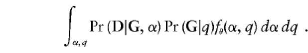So the retrospective likelihood, for example, under this mixed model, looks like

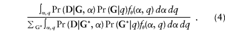In principle, maximum-likelihood estimates for β and θ based on (4) can be calculated using the Newton-Raphson algorithm and numerical integration. In practice, this will often be very difficult to implement. However, if α and q are assumed to be discrete, then the integrals in (4) become sums, and calculation of maximum-likelihood estimates becomes more tractable. On the other hand, discrete distributions may require more parameters than continuous distributions.

In order to investigate the feasibility and efficiency of the mixed-model likelihoods, we examined the prospective, retrospective, and joint likelihoods based on the mixed model (3) presented in the previous section. These likelihoods have the form:

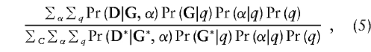where C is the appropriate conditioning event. Assuming that the true distribution of D, G, and the unobserved α and q has the form of (3), the prospective, retrospective, and joint likelihoods all have an expected score of zero at the true parameter values. It follows that maximum-likelihood estimates based on (5) will be consistent. Note that if α and q are not independent, then the prospective likelihood also involves the Pr(q) terms; when α and q are independent, the terms involving the allele frequency drop out.

Table 3 shows the relative efficiencies of the mixed-model likelihoods. These were based on direct calculations of the expected information evaluated at the true parameters. For the cases of heterogeneity in α or q alone, a reduced mixed model—which only modeled heterogeneity in the appropriate parameter—was used. So, for example, while the mixed-model retrospective likelihood involved eight parameters in the case of heterogeneity in α and q, it only involved five in the cases of heterogeneity in α alone or heterogeneity in q alone.

Table 3.

Efficiency of the Standard Conditional and Mixed-Model Prospective and Retrospective Likelihoods Relative to the Mixed-Model Joint Likelihood

	Likelihood
Conditions	Conditional	Prospective	Retrospective
	Heterogeneity in q Alonea
Genetic odds ratio = 20	.43	1.01	.95
Genetic odds ratio = 2	.66	1.00	.92
	Heterogeneity in α Aloneb
Genetic odds ratio = 20	.98	.83	.99
Genetic odds ratio = 2	.83	.78	.81
	Heterogeneity in Both α and qc
Genetic odds ratio = 20:
α and q independent	.92	.99	.99
α and q positively correlated	.89	.99	.99
α and q negatively correlated	.94	1.00	.98
Genetic odds ratio = 2:
α and q independent	.93	.96	.93
α and q positively correlated	.90	.96	.95
α and q negatively correlated	.92	.93	.92

^aΔα=2.30; Pr(α=α₁)=0.25; population rate =0.10; q=0.05.

^bq₀=0.0098; q₁=0.0902; Pr(q=q₁)=0.50; population rate =0.10.

^cq₀=0.0098; q₁=0.0902; Pr(q=q₁)=0.50; Δα=2.30; Pr(α=α₁)=0.25; population rate = .10. For the independent case, η=0.00; for the positive correlation case, η=2.30; and for the negative correlation case, η=-2.30.

In practice, we might try to fit a model with heterogeneity in both α and q to data from a distribution which is heterogeneous in only one (or neither) factor. In this case, the expected information at the true parameters for the fully heterogeneous likelihood is singular, so there may be problems with the convergence of estimates.

The efficiency of standard conditional likelihood is not markedly worse than that of the mixed joint likelihood, except in the case of heterogeneity in q alone. The prospective and retrospective likelihoods performed about as well as the joint likelihood for all the cases considered here. In fact, the prospective likelihood was slightly more efficient than the joint likelihood in the case of heterogeneity in q alone. This was possible because the prospective likelihood only involved two parameters, whereas the joint likelihood involved five (in fact, in the absence of heterogeneity in α, the homogeneous prospective likelihood gives consistent parameter estimates).

The asymptotic variances for the estimates of the nuisance parameters describing the distribution of α and q were often very large. For example, when the genetic odds ratio was 2, the joint-likelihood estimates for α₀ and Δα were >1,000 times less efficient than the estimates for β. For larger genetic odds ratios, the estimates for α and α₀ were considerably more efficient, but the estimates for q₀ and q₁ remained relatively inefficient (data not shown). However, the inefficiency in the estimates of the nuisance parameters does not effect the consistency or efficiency of the estimate for the log odds ratio discussed above.

Discussion

The calculations reported in this paper suggest that the prospective, joint, and retrospective likelihoods will generally be more efficient than the standard conditional likelihood for analyzing family-based studies of candidate genes in the case of homogeneous baseline rates and allele frequencies. The advantages and drawbacks of these likelihoods examined are summarized in table 4.

Table 4.

Summary of the Properties of the Four Likelihoods

Likelihood	Drawbacks	Advantages
Standard conditional	Disease (and genotype) concordant sets noninformative. Only yields information on genetic odds ratio, not absolute penetrance.	Not affected by heterogeneity in q. Do not have to explicitly model ascertainment.
Prospective	Must explicitly model ascertainment rule. Sensitive to heterogeneity in baseline rates.	Not affected by heterogeneity in q. Can be more efficient than standard conditional likelihood. Yields information on both relative risk and baseline rates.
Retrospective	Sensitive to heterogeneity in baseline rates and allele frequencies. Low power for estimating absolute penetrances.	Do not have to explicitly model ascertainment rule. More efficient than standard conditional and prospective likelihood for estimating relative risk.
Joint	Must explicitly model ascertainment rule. Sensitive to heterogeneity in baseline rates and allele frequencies.	Most efficient of all.

In particular, the retrospective likelihood avoids the difficulties of modeling ascertainment correction when the families are not obtained in a population-based manner—as long as ascertainment only depends on a sibship’s phenotypes. Some recent linkage studies (e.g., Easton et al. 1995) analyzed families with four or more cases and a high LOD score using MOD-score techniques (the linkage analog to the retrospective likelihood). In this case, the MOD-score/retrospective likelihood does not correct for ascertainment, because ascertainment depends on the joint distribution of phenotypes and genotypes (through the LOD-score requirement). MOD-score analysis of sibships sampled on the basis of high LOD scores substantially overestimates the penetrance in carriers (Siegmund et al. 1999).

Several other cautionary remarks are in order. First, if there is between-family heterogeneity in baseline rates, then a likelihood that assumes a homogeneous baseline rate may provide a biased estimate of the genetic odds ratio. Similarly, heterogeneity in allele frequencies can lead to bias in parameter estimates based on the homogeneous model. This is not a novel result; there is no reason to expect that a maximum-likelihood estimate, , should converge to the true β in the presence of an omitted covariate which is related to disease (such as when there is heterogeneity in α). For example, in the case of unconditional logistic regression with an individual-specific covariate X that is marginally independent of a measured dichotomous exposure Z, converges to

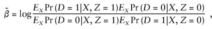an odds ratio based on the marginal probability Pr(D|Z) (Gail 1984; Greenland 1987). Because of this, will be biased towards the null even when X and Z are independent (Hauck 1991). In the case of heterogeneity in family-specific baseline odds, for the four conditional likelihoods discussed here does not, in general, converge to the analogous value

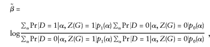where 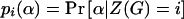. In fact, when there is heterogeneity in α and α and q are independent, is further biased towards the null, that is, .

We should note here that the estimate , which is based on the log-linear model , will converge to the true β even in the case of heterogeneity in α and q—as long as α and q are independent. The estimate still will not converge to β when α and q are correlated (confounding caused by population stratification). The main drawback to the log-linear model is computational; the maximum-likelihood estimates must be constrained so that .

The gist of the two preceding paragraphs is that care must be taken when interpreting the estimated odds ratio in the presence of heterogeneity. This quasimarginal odds ratio may not be of primary importance. If investigators are mostly interested in determining whether a major gene plays a role in increasing risk in individuals and are less interested in how this increase in risk plays out in a large population, then the conditional genetic odds ratio β is more relevant than the marginal odds ratio (Greenland 1987; Greenland 1999).

Random-effects (mixed) models can correctly estimate β in the presence of between-family heterogeneity while avoiding proliferation of family-specific parameters. The mixed-model joint likelihood can even be more efficient than the conditional likelihood, and other parameters can be estimated by use of the mixed-model likelihoods, but not by use of the standard conditional likelihood. However, the efficiency gains over the standard conditional likelihood were negligible in the cases we examined, and the asymptotic variances for nuisance parameters (like allele frequencies) were large.

The dichotomous random-effects models for heterogeneity in baseline odds and allele frequencies presented in this paper may differ markedly from the real variation in those parameters. However, unless we have evidence that there is no heterogeneity or that the heterogeneity is small enough to have little effect, it may be better to use a misspecified model that takes some form of heterogeneity into account than to fit a model which ignores it completely. In principle, a random-effects model allows us to test for the presence of heterogeneity in baseline odds and/or allele frequencies. If there is no evidence of heterogeneity, then a homogeneous likelihood can be used. If there is evidence of heterogeneity in one or both factors, investigators can fit a random-effects model, which need not take a dichotomous form—investigators can also use multipoint discrete or continuous models, or they can estimate the random-effect distribution nonparametrically (Laird 1978). The properties of this two-step approach (such as test size and power) as well as the properties of more sophisticated random-effects models are subjects for future research.

Second, the likelihoods presented here assume that the baseline risk within a family is characterized by a single parameter α. In most chronic diseases, the baseline risk varies in a complex manner with age, gender, race, calendar time, and (perhaps) other factors. A major advantage of the conditional likelihood for case-control data is that all such dependencies are eliminated by appropriately matching on such factors in the selection of controls (Lubin and Gail 1985). Practical applications of the other likelihoods would therefore require one to model such effects. It is unclear whether their efficiency gain, relative to the prospective likelihood, would be as impressive, once the need for many such additional parameters was allowed for.

The methods presented here can be extended to include failure-time models, which can take the variation in baseline risk with age into account. For example, the ARCAD (analysis of risk corrected for ascertainment and using age at diagnosis) of Le Bihan et al. (1995) is essentially what we called the “joint” likelihood extended to the context of failure-time analysis (they also allow for non–nuclear family data and subjects with missing genotypes). For the retrospective likelihood, if we assume (a) that the hazard rate for an individual has some parametric form λ(t,G), (b) that censoring time is independent of genotype, and (c) that the censoring times for individuals in a sibship are independent, then we can write Pr(G|D,t) as follows:

Under assumptions (b) and (c), the censoring process cancels out of this fraction. The hazard λ(t_i,G_i) can be modeled parametrically or semiparametrically (e.g., assuming proportional hazards and using a step function for λ(t)). We are currently investigating the properties of prospective, retrospective, and joint likelihoods based on failure-time models. We are particularly interested in the feasibility of using frailty models to account for differences in baseline rates.

Finally, within-family dependencies may be more complicated than the model presented above, where families share an unobserved baseline risk. Such residual within-family dependencies can arise because of other genes (major genes or polygenes) or because of unmodeled environmental factors. When these factors are correlated with the candidate gene, ignoring them can lead to biased estimates of the parameters of the model using any of the proposed likelihoods. For example, if the candidate gene is inert but is in linkage disequilibrium with a causal gene, then (a) it will appear to be related to disease and (b) the assumption that the phenotypes of siblings are independent given their (observed) genotypes will be violated. Point (a) changes our interpretation of the results, and point (b) implies that tests of β=0 will have the wrong size. On the other hand, if the unmeasured risk factor is independent of genotype given disease status, then ignoring the risk factor will not induce a bias (Whittemore 1978). We are investigating further the effect of other unmeasured risk factors on the estimates for the odds ratio or relative risk and the parameter-variance estimates. In particular, if one family member’s phenotype has a direct causal influence on another’s, then regressive models may account for this influence (Bonney 1986).

References

- Bonney GW (1986) Regressive logistic models for familial disease and other binary traits. Biometrics 42:611–625 [PubMed]
- Breslow NE, Day NE (1980) Statistical methods in cancer research. Vol 1: The analysis of case-control studies. International Agency for Research on Cancer, Lyon [PubMed] [Google Scholar]
- Claus EB, Risch N, Thompson WD (1991) Genetic analysis of breast cancer in the cancer and steroid hormone study. Am J Hum Genet 48:232–242 [PMC free article] [PubMed]
- Easton DF, Bishop DT, Ford D, Crockford GP, Breast Cancer Linkage Consortium (1993) Genetic linkage analysis in familial breast and ovarian cancer: Results from 214 families. Am J Hum Genet 52:678–701 [PMC free article] [PubMed]
- Easton DF, Ford D, Bishop DT, Breast Cancer Linkage Consortium (1995) Breast and ovarian cancer incidence in BRCA-1 mutation carriers. Am J Hum Genet 56:265–271 [PMC free article] [PubMed]
- Elston RC, Bonney GE (1984) Sampling considerations in the design and analysis of family studies. In: Rao DC (ed) Genetic epidemiology of coronary heart disease: past, present, and future. Alan R Liss, New York, pp 349–371 [Google Scholar]
- Gail MH, Wieand S, Piantadosi S (1984) Biased estimates of treatment effect in randomized experiments with nonlinear regressions and omitted covariates. Biometrika 71:431–444 [Google Scholar]
- Gail MH, Pee D, Benichou J, Carroll R (1999) Designing studies to estimate the penetrance of an identified autosomal dominant mutation. Genet Epidemiol 16:15–39 [DOI] [PubMed]
- Gauderman WJ, Faucett CL (1997) Detection of gene-environment interactions in joint segregation and linkage analysis. Am J Hum Genet 61:1189–1199 [DOI] [PMC free article] [PubMed]
- Greenland S (1987) Interpretation and choice of effect measures in epidemiologic measures. Am J Epidemiol 125:761–768 [DOI] [PubMed]
- Greenland S (1999) A unified approach to the analysis of case-distribution (case-only) studies. Stat Med 18:1–15 [DOI] [PubMed] [Google Scholar]
- Hauck WW, Neuhaus JM, Kalbfleisch JD, Anderson S (1991) A consequence of omitted covariates when estimating odds ratios. J Clin Epidemiol 44:77–81 [DOI] [PubMed]
- Hodge SE and Elston RC (1994) Lods, wrods, and mods: the interpretation of lod scores calculated under different models. Genet Epidemiol 11:329–342 [DOI] [PubMed]
- Laird N (1978) Nonparametric maximum likelihood estimation of a mixing distribution. J Am Stat Assoc 73:805–811 [Google Scholar]
- Lander ES, Schorck NJ (1994) Genetic dissection of complex traits. Science 265:2037–2048 [DOI] [PubMed]
- Le Bihan C, Moutou C, Brugieres L, Feunteun J, Bonaiti-Pellie C (1995) ARCAD: a method for estimating age-dependent disease risk associated with mutation carrier status from family data. Genet Epidemiol 12:13–25 [DOI] [PubMed]
- Liang KY, Rathouz PJ, Beaty TH (1996) Determining linkage and mode of inheritance: Mod scores and other methods. Genet Epidemiol 13:575–593 [DOI] [PubMed]
- Lubin JH, Gail MH (1985) Biased selection of controls for case-control analyses of cohort studies. Biometrics 40:63–75 [PubMed] [Google Scholar]
- Prentice RL, Pyke R (1979) Logistic disease incidence models and case-control studies. Biometrika 66:403–411 [Google Scholar]
- Siegmund K, Gauderman WJ, Thomas DC (1999) Gene characterization using high-risk families: a sensitivity analysis of the MOD score approach. Am J Hum Genet Suppl 65:A398 [Google Scholar]
- Struewing JP, Hartge P, Wacholder S, Baker SM, Berlin M, McAdams M, Timmerman MM, et al (1997) The risk of cancer associated with specific mutations of BRCA1 and BRCA2 among Ashkenazi Jews. N Engl J Med 336:1401–1408 [DOI] [PubMed]
- Whittemore AS (1978) Collapsibility of multidimensional contingency tables. J R Statist Soc B 40:328–340 [Google Scholar]
- Witte JS, Gauderman WJ, Thomas DC (1999) Asymptotic bias and efficiency in case-control studies of candidate genes and gene-environment interaction: basic family designs. Am J Epidemiol 149:693–705 [DOI] [PubMed]