Multipoint Estimation of Genetic Maps for Human Trisomies with One Parent or Other Partial Data

Abstract

Centromeric-mapping methods have been used to investigate the association between altered recombination and meiotic nondisjunction in humans. For trisomies, current methods are based on the genotypes from a trisomic offspring and both parents. Because it is sometimes difficult to obtain samples from both parents and because the ability to use sources of DNA previously not available (e.g., stored paraffin-embedded pathological samples) has increased, we have been interested in creating similar maps for trisomic populations in which one of the parents of the trisomic individual is unavailable for genotyping. In this paper, we derive multipoint likelihoods for both missing-parent data and conventional two-parent data. We find that likelihoods for two-parent data and for data generated without a sample from the correctly disjoining parent can be maximized in exactly the same way but also that missing-parent data has a high frequency of partial data of the same sort produced by intercross matings. Previously published centromeric-mapping methods use incorrect likelihoods for intercross matings and thus can perform poorly on missing-parent data. We wrote a FORTRAN program to maximize our multipoint likelihoods and used it in simulation studies to demonstrate the biases in the previous methods.

Introduction

Recent work on the etiology of trisomy has documented a strong association between altered recombination and meiotic nondisjunction in both humans and Drosophila (Warren et al. 1987; Sherman et al. 1991; Sherman et al. 1994; Koehler et al. 1996). As reviewed by Koehler et al. (1996), genetic maps of the nondisjoined chromosome have been used to investigate recombination patterns for trisomies 16, 18, and 21 and the sex chromosomes. Similar methods have also been used to study the behavior of recombination in uniparental disomy 15 (Mascari et al. 1993; Robinson et al. 1993) and in human ovarian teratomas (Chakravarti et al. 1989; Deka et al. 1990). We have been interested in creating maps for trisomic populations in which one of the parents of the trisomic individual is unavailable for genotyping. For example, since the majority of trisomies result in spontaneous abortions, only pathological samples—including maternal and fetal tissue samples—are generally available for study. But current centromeric-mapping methods (e.g., Chakravarti et al. 1989, Morton et al. 1990) assume data from both parents are available.

In this paper, we derive multipoint likelihoods for both missing-parent data and conventional two-parent data. We find that likelihoods for two-parent data and for data generated without a sample from the correctly disjoining parent are the same up to constants and thus can be maximized in exactly the same way. However, missing-parent data has a very high frequency of partial data of the same sort produced by intercross matings, and the likelihoods for this type of data are not quite correct in the previously published centromeric-mapping methods. We describe our FORTRAN program, NDJMap, which maximizes our likelihoods using an estimation-maximization (EM) algorithm (Little and Rubin 1987) and present simulation results demonstrating the bias in previous methods. The bias is not substantial for most of the realistic two-parent data sets we tried, but is a problem in the missing-parent data sets.

Data for Human Trisomy Mapping

The basic unit of data for a genetic map of a nondisjoined chromosome is a trisomic offspring along with one or two parents. These two or three individuals are genotyped for markers along the trisomic chromosome. Typically it is not difficult to establish the parent of origin of the extra chromosome if enough markers are typed. We will call the parent of origin of the extra chromosome the “nondisjoining parent” (NDJP) and the other parent the “correctly disjoining parent” (CDJP). In a meiosis II nondisjunction, the two chromosomes inherited from the nondisjoining parent are sister chromatids and are identical by descent at the centromere. In a meiosis I nondisjunction, the two chromosomes are not sister chromatids and are not identical by descent at the centromere. Because of recombination, the two chromosomes may or may not be identical by descent at loci other than the centromere. At any given locus, the two chromosomes are described as “reduced to homozygosity” (coded as “R”) if they are identical by descent, and “nonreduced” (coded as “N”), if they are not identical by descent. The distance between two loci is usually parameterized in terms of y, which can be defined as the probability of being in state N at the second locus given that the half-tetrad is in state R at the first locus. If there is no chiasma interference, , where θ is the usual recombination fraction between the two loci. When the distance is small, y≈2θ. In nondisjunction mapping, the order of markers is not generally an issue, since the order is established in the normal map, so “creating a map” means estimating the y values for all the intervals and possibly converting those values to genetic distances. Chakravarti and Slaugenhaupt (1987) give a quite complete review of this terminology and the related mathematical models, extending a large body of previous work (e.g., Cote and Edwards 1975; Morton and Maclean 1984; Shahar and Morton 1986).

A completely informative marker provides unequivocal information about whether the two chromosomes are R or N at the locus. If all markers are completely informative, creating a genetic map is straightforward under the assumption of no interference (e.g., Chakravarti and Slaugenhaupt 1987), and can also be handled under a χ² model of interference (Zhao and Speed 1998). Unfortunately, not all markers are fully informative in typical human data. Table 1 shows our coding of the marker information status, given various parental genotypes, when both parents are available for genotyping. If the nondisjoining parent is homozygous, the marker is completely uninformative, which we code as “U.” Untyped markers can also be considered uninformative, as long as any decisions about whether to type markers are independent of what the true state is (N or R) at that marker. Intercross matings can produce an R or an X (D or X in the notation of most previous work). A marker status of X indicates that the marker is partially informative; we do not have unequivocal information about whether the true state is N or R, but some information is added because the probability of observing an X depends on what the true state is. For example, if the results for three ordered loci are NUN, we know that the middle marker’s true state is likely to be N, simply because it is flanked by two Ns. But if, instead, we observe NXN, it is even more likely that the true state at the middle marker is N, because a true N is more likely to be observed as an X than is a true R. Exact probabilities for these events are described in the Multipoint Likelihoods section below.

Table 1.

Coding of the Marker Status, Given Various Parental Genotypes When Both Parents Are Genotyped

NDJP Genotype	CDJP Genotype	Child Genotype	Marker Status
ab	cd	abc, abd	N
		aac, bbc, aad, bbd	R
ab	bc	abc, abb	N
		aab, aac, bbb, bbc	R
ab	cc	abc	N
		aac, bbc	R
ab	bb	abb	N
		bbb, aab	R
ab	ab	abb, aab	X
		aaa, bbb	R (D)
aa	Anything	Anything	U

Table 2 shows our coding of the marker status, given various parental genotypes, when one parent is unavailable for genotyping. It is fairly common for the CDJP (who in most cases is the father) to be unavailable and less common for the NDJP to be missing. In the tables we have used X to indicate any partially informative marker. In fact, the information provided by an X (i.e., the relative probabilities that the X represents a true N or R) depends on the type of data (two-parent, missing CDJP, missing NDJP); this is discussed in detail in the next section. While Xs are fairly uncommon in two-parent data—as long as the markers are reasonably informative—they can be quite common in missing-parent data. For example, for a marker with five equally frequent alleles (assuming random mating), the probability of observing an X, given that the true state is N, is only .064 for two-parent data but is .32 for missing-CDJP data. For a marker with two equally frequent alleles, the corresponding probabilities are .25 and .5. Note that the issues of missing parents and partially informative data do not arise in either ovarian teratomas or uniparental disomy, both of which produce only N, R, and U data.

Table 2.

Coding of the Marker Status, Given Various Parental Genotypes One Parent Is Missing

NDJP Genotype	CDJP Genotype	Child Genotype	Marker Status
ab	Missing	abc	N
		aac, bbc, aaa, bbb	R
		aab, abb	X
aa	Missing	Anything	U
Missing	aa	aab, abc	N
		abb, aaa	X
Missing	ab	acd, bcd, abc	N
		aaa, bbb, abb, aab, acc, bcc	X

Multipoint Likelihoods

After coding the marker data as described in table 1 and/or table 2, the data for a given trisomic individual will consist of a string of ordered loci, e.g. NURRXRXXU. We assume that the leftmost locus represents the centromere, so that we are mapping one arm of a chromosome at a time. We further assume that the centromeric marker is fully informative (no Xs or Us allowed in the first spot), so that we know whether this chromosome is the result of a meiosis I or a meiosis II nondisjunction. In practice, this is generally accomplished by typing several closely-spaced markers as close to the centromere as possible. The likelihood of observing any given string of marker data can be written as a function of the y parameters between each pair of markers.

The basic mathematical model we work with is that at every locus on the chromosome, including those where we have markers and those where we do not, there exists an unseen true state of N or R. By assuming no crossover interference, we can model the process of transitions between these two states, as we move along the chromosome, as a continuous-time Markov process. That is, the no-interference assumption gives the Markov property that the probability of a transition in any interval of the chromosome does not depend on what has happened in any other interval. The Markov process starts at the centromere in state N for a meiosis I nondisjunction and in state R for a meiosis II nondisjunction. Between any two markers, the probabilities of various types of transitions can be calculated as a function of the y parameter for that interval. If we are in state R, the probability of still being in state R at the next marker is 1-y, and the probability of switching to state N is y. If we are in state N, the probability of still being in state N at the next marker is 1-y/2, and the probability of switching to state R is y/2 (Chakravarti and Slaugenhaupt 1987). The string of data we actually observe is a random function of the underlying Markov process. This is known as a hidden Markov process.

Let the vector W be the string of observed data, and let T be the string representing the true state of the Markov process at each marker. The likelihood that we want to compute is P(W), which can be calculated by conditioning on the underlying true state by use of the formula

The probabilities of each true state, P(T=t), can be written simply as a function of the interval-by-interval probabilities given above. For example, the probability of NNRRRN is (1-y₁/2)(y₂/2)(1-y₃)(1-y₄)(y₅), where y₁, y₂,…y₅ are the y parameters for the five intervals. Note that there is no term in this likelihood for the probability that the first marker is N; the likelihood is really the conditional probability that markers 2–6 are NRRRN, given that the first marker is N. The probabilities P(W=w|T=t) seem at first to be complicated but in fact are fairly simple, because they are independent for each locus. That is, given the true underlying string, what we actually observe at each locus depends only on the true status at that locus and not on the true status at any other loci. For example, if we have both parents available and the true state is N at a given locus, we observe X instead of N if and only if the parents are an intercross mating at that locus, an event that clearly does not depend on the true state of the offspring at any other locus. So, to compute P(W=w|T=t) for a string of data, we just need to calculate all the one-marker conditional probabilities—for example, P(observe X | true state is N). Then, we multiply these probabilities for all the markers in the string, omitting only the first marker, whose state we are conditioning on. These probabilities depend on the type of data—two-parent, missing-CDJP, or missing-NDJP—so we discuss each case separately. In the following exposition, we omit, for clarity, the probability that markers are untyped, but it is not difficult to add that to the models shown, and it does not affect our results.

If both parents are available for genotyping and the mating type at this marker is not an intercross (i.e. we cannot observe an X), the probabilities are simply

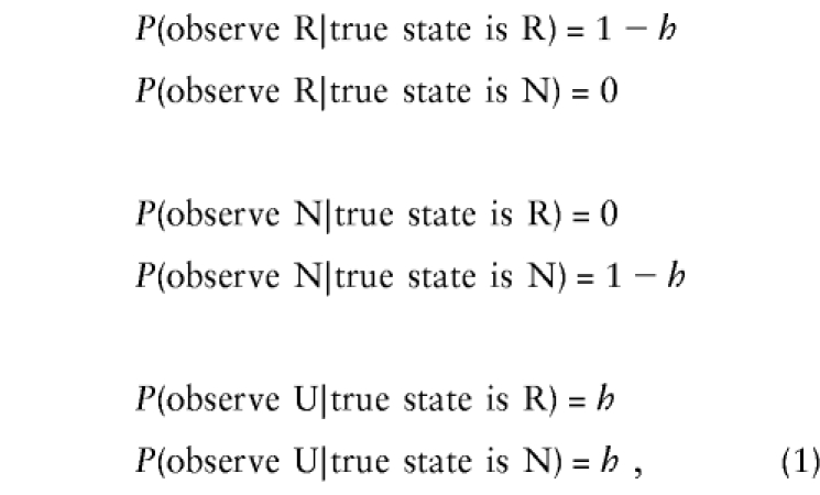where h is the probability that the nondisjoining parent is homozygous at the marker. This parameter does not need to be known or estimated, however, because all that matters in the likelihood is the ratio of each pair of lines above—for example, P(observe R | true state is R) / P(observe R | true state is N). To demonstrate this in a simple example: suppose we want to find the likelihood of the string RU. We calculate

The (1-h) and h are constant in both terms, so they do not matter in maximizing the likelihood. Thus, for the purpose of maximizing the likelihood, the probabilities in equation set (1) can be treated equivalently as

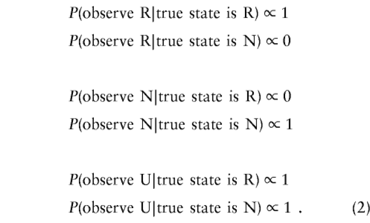If we have both parents available but also have an intercross mating at this marker, the probabilities are

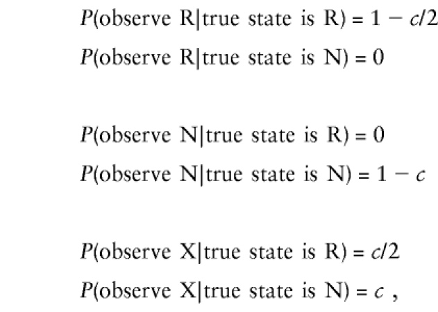where c is the probability that the parental mating type is an intercross at the marker. The equation P(observeX|truestateisR)=c/2 is a result of the information in table 1 and the assumption that the allele inherited from the CDJP is independent of the alleles inherited from the NDJP. If we again eliminate parameters that are constant in the likelihood, we have

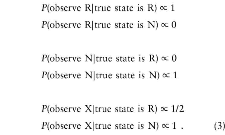Since this matches equation set (2), we have the convenient result that we need only one set of equations for both intercross and nonintercross cases. Combining equation sets (2) and (3), we get

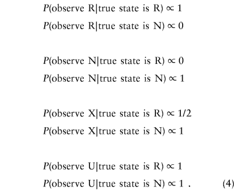Even more conveniently, we have found that equation set (4) is also correct for data where the CDJP is not genotyped. In that case the full probabilities are

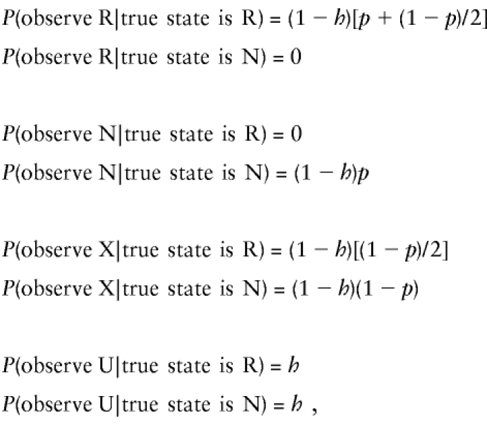where p is the probability that the CDJP contributes an allele that is different from either of the alleles of the NDJP, given that the NDJP is a heterozygote. That is, looking at table 2, if the NDJP is a heterozygote and the true state is N, we observe an N if and only if the CDJP contributes an allele different from those of the NDJP (probability p, as defined above). If the NDJP is a heterozygote and the true state is R, we observe an R if the CDJP contributes a different allele from those of the NDJP (probability p), but also if the CDJP contributes an allele that matches the one owned but not contributed by the NDJP (probability (1-p)/2). The probability p can be estimated from population allele and genotype frequencies, but we do not need to do so because, like h and c, it is constant in the likelihood.

Thus, we can use equation set (4) to compute likelihoods in exactly the same way for two-parent data and for missing-CDJP data, without needing to know which of those two types of data we are dealing with and without having to know anything about mating types or genotype frequencies. An immediate implication of this result is that it is, after all, hypothetically appropriate to use existing centromeric-mapping methods with data in which the CDJP is missing. However, because missing-CDJP data has a high frequency of Xs, as compared with two-parent data, we found that the existing methods estimated biased maps (see Simulation Results).

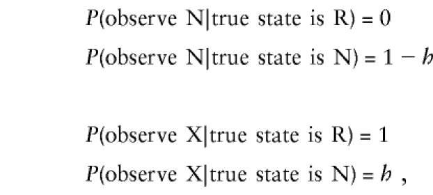
The case where the NDJP (generally the mother) is missing is not as simple, and genotype frequencies are required to calculate the likelihood. The necessary probabilities when the CDJP is homozygous are

and, when the CDJP is heterozygous, are

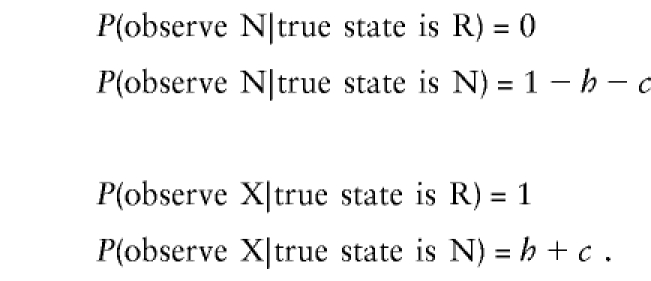Note that the frequencies h and c will be different for each marker, depending on the population genotype frequencies at that marker. To use such chromosomes in the creation of maps therefore requires estimates of h and c for each marker, and also a designation of which strings of data are from missing-NDJP cases.

Putting together all of the above, we can write the likelihood of any string of markers for any of the three types of data we want to consider. Except in the case of missing-NDJP data, we do not need estimates of any allele frequencies or other nuisance parameters. However, the likelihoods can be extremely complicated. There is one parameter for each interval along the chromosome, and, if a given string has a total of k Us and Xs, there will be 2^k possible true strings, so the likelihood will be the sum of 2^k terms. Then the likelihoods must be multiplied for all of the strings of data. Maximizing such a likelihood directly is possible when there are only a few intervals, but the computation time rises exponentially with the number of intervals and becomes impractical quite quickly. The likelihood can be maximized quite easily, however, using the EM algorithm. This iterative algorithm starts with a user-supplied guess at the parameter values. The next step (the expectation step, or E-step) is to compute the expected number of each possible value of T, given the observed data and the guessed parameter values. The maximization step, or M-step, then maximizes the likelihood of this “expected data” and thus generates new estimates of the parameters. These parameter estimates are fed back into the E-step, and the algorithm iterates until it converges. We implemented an EM algorithm to maximize our likelihoods in a FORTRAN program called NDJMap. A detailed description of our EM algorithm, including an example, is given in the appendix. The EM algorithm also allows for easy calculation of approximate standard errors of estimates; we have implemented this feature in our program using the method of Meng and Rubin (1991). NDJMap handles only two-parent data and missing-CDJP data, but it would be straightforward to add the ability to handle missing-NDJP data by means of the probabilities given above and an extra data file with the needed genotype frequencies.

Theoretical Comparison to Previous Methods

Existing methods for centromeric mapping are implemented in the software packages DSLINK (Halloran and Chakravarti 1987; Chakravarti et al. 1989) and TETRAD/MAP/Map+ (Morton and Andrews 1989; Morton et al. 1990; Collins et al. 1996). There are two important differences in basic estimation methods among the programs: method of handling Xs and method of incorporating multipoint information. Our method (implemented in NDJMap) incorporates multipoint information by maximizing a multipoint likelihood, which is the statistically optimal method under the assumption of no interference. DSLINK also maximizes a multipoint likelihood, assuming no interference. The authors of TETRAD have argued that, since the assumption of no interference is known to be wrong, it is more appropriate to estimate all pairwise distances between markers and then combine these using “multiple pairwise linkage” methods that incorporate interference assumptions. Thus, TETRAD computes the distances between all pairs of markers (both adjacent and nonadjacent pairs), and MAP combines the pairwise estimates to produce a final map. The program Map+ is a newer implementation that combines these calculations into one program. The issue of whether multipoint maximum likelihood or multiple pairwise linkage is a better method of incorporating multipoint information is an extremely complicated one, and we will not attempt to resolve it in this paper. We are primarily interested in the method of handling Xs, since that bears on the appropriateness of the methods for missing-parent data. (In fact, missing-parent data does not have Us at all, except for untyped markers).

DSLINK handles intercross matings by using the information whenever the marker can be recorded as an R (D), but ignoring Xs. This is quite clearly a biased procedure. For example, in meiosis I cases, all chromosomes start with N. If the second marker is an intercross, it goes into the calculation only if it is an R and is thrown out if the true value is N (recorded as X). Thus, the program uses an excess of NR strings, biasing the estimate of y upward. The bias is in the opposite direction for meiosis II cases.

To handle Xs, TETRAD calculates the likelihoods of the strings NX, XN, RX, and XR, since it is only calculating two-marker likelihoods. The likelihood of NX is calculated the same way we calculate it, as

The likelihood of RX is calculated analogously. The likelihood of XN is assumed to be equal to the likelihood of NX. In conventional (noncentromeric) genetic mapping, this kind of symmetry is correct, because, in the absence of any marker data, at every locus, the chromosome being examined is equally likely to be identical by descent with the chromosomes of either grandparent. That is, from a mathematical point of view, the underlying Markov chain of recombination states is in its limiting distribution at every point on the chromosome. But centromeric mapping is different, because, in fact, there is a point on the chromosome (the centromere) where the distribution is not the limiting distribution of 2/3 Ns and 1/3 Rs. Making the symmetry assumption in centromeric mapping is mathematically equivalent to assuming that the a priori probability of an N at each locus is 2/3. For intervals near the telomere, where the underlying Markov chain is approaching its limiting distribution, the symmetry assumption should be nearly correct, but it is wrong near the centromere if one is mapping a pure meiosis I or pure meiosis II population. TETRAD does not calculate a likelihood for XX intervals, presumably because under the symmetry assumption this likelihood does not depend on y. It is not clear whether TETRAD calculates likelihoods for what its authors call DX and XD intervals (see, e.g., table 4 of Collins et al. 1996). Thus, TETRAD is calculating slightly incorrect likelihoods for XN, XR, and XX. Unfortunately, these likelihoods cannot just be corrected. It is actually not possible to correctly calculate likelihoods for those pairs in centromeric mapping, because any likelihood for a string starting with X implicitly makes some assumption about the a priori probabilities of N and R, which in turn depend on the genetic map. It was this realization that pushed us into a multipoint maximum likelihood approach to mapping, even though there are very reasonable arguments for the multiple pairwise linkage approach.

Table 4.

Mean (SD) of Estimated y- Values for Simulated Data with CDJP Not Genotyped^[Note]

	Mean Estimated y (SD) at Interval
Data Type and Program Used	1	2	3	4	5	6	7	8
Meiosis I data:
NDJMap	.198 (.036)	.200 (.042)	.202 (.040)	.200 (.039)	.201 (.039)	.202 (.039)	.198 (.038)	.199 (.040)
TETRAD	.198	.190	.197	.199	.204	.206	.203	.204
DSLINK	.274 (.085)	.234 (.085)	.221 (.075)	.206 (.072)	.208 (.070)	.218 (.063)	.234 (059)	.360 (.056)
Meiosis II data:
NDJMap	.200 (.025)	.200 (.031)	.199 (.032)	.201 (.035)	.199 (.033)	.199 (.037)	.200 (.037)	.200 (.038)
TETRAD	.200	.228	.222	.219	.214	.213	.211	.209
DSLINK	.146 (.037)	.162 (.047)	.169 (.056)	.173 (.052)	.182 (.053)	.194 (.052)	.220 (.51)	.322 (.047)

Note.—Intervals are listed cen→tel. Simulation parameters are for markers with five equally frequent alleles. True value of y=.2 for all intervals. Total sample size is 400,000 chromosomes.

Simulation Results

We did fairly extensive simulation studies using TETRAD, DSLINK, and NDJMap. The studies were designed for three purposes: (1) to demonstrate the existence of the biases we claim are present in TETRAD and DSLINK, (2) to see whether those biases are large enough to make any practical difference, and (3) to validate NDJMap. We simulated data by first setting the “centromeric marker” to be N or R and then simulating the rest of the true underlying string of Ns and Rs, assuming no interference. Then, for each marker except the first, we simulated the observed data as a function of the true state using the probabilities given in the Multipoint Likelihoods section above. Simulations used a single chromosome arm, spanned by 7 to 20 equally spaced markers. We tested values of y ranging from .05 to .4. We ran meiosis I and meiosis II data separately and two-parent and missing-CDJP data separately, in order to clearly assess any problems that might be limited to one kind of data. Most simulations used a single large data set of 10,000 chromosomes or 400,000 chromosomes, though some used 1,000 data sets of 400 chromosomes so that we could look at variances of estimates in addition to biases. In analyzing the simulated data, we used TETRAD without MAP because we were interested in an uncomplicated comparison of handling of Xs. We present selected simulation results here, to highlight the most important issues.

Table 3 gives results for what should be easy data for all the programs: both parents genotyped on markers with five equally frequent alleles (random mating assumed). There are nine markers, and the true value of y is .2 (∼10 cM) in each interval. For NDJMap and DSLINK, we ran 1,000 data sets of 400 chromosomes. For TETRAD, we ran the same data as a single data set of 400,000 chromosomes, for reasons discussed below. The table shows mean y estimates to three decimal places, so that patterns of bias can be seen clearly—but it should be pointed out that, at most, two decimal places are of practical interest. We also show standard deviations of the estimates, computed over the 1,000 replicates. Standard errors (found by dividing the standard deviations by the square root of 1,000) are on the order of .001. The only bias of practical importance visible in these runs is a severe overestimation of the last interval by DSLINK. DSLINK also has a somewhat higher variance than does NDJMap.

Table 3.

Mean (SD) of Estimated y-Values for Simulated Data with Both Parents Genotyped^[Note]

	Mean Estimated y (SD) at Interval
Data Type and Program Used	1	2	3	4	5	6	7	8
Meiosis I data:
NDJMap	.202 (.033)	.198 (.036)	.201 (.032)	.202 (.032)	.200 (.032)	.200 (.032)	.200 (.032)	.201 (.033)
TETRAD	.202	.195	.199	.201	.199	.200	.200	.201
DSLINK	.204 (.045)	.196 (.046)	.196 (.041)	.197 (.043)	.195 (.041)	.197 (.041)	.207 (.045)	.280 (.041)
Meiosis II data:
NDJMap	.202 (.022)	.199 (.025)	.200 (.028)	.201 (.027)	.199 (.029)	.200 (.029)	.201 (.031)	.199 (.031)
TETRAD	.202	.202	.203	.203	.201	.201	.201	.200
DSLINK	.198 (.030)	.197 (.034)	.201 (.037)	.203 (.036)	.204 (.040)	.207 (.039)	.216 (.040)	.296 (.042)

Note.—Intervals are listed cen→tel. Simulation parameters are for markers with five equally frequent alleles. True value of y=.2 for all intervals. Total sample size is 400,000 chromosomes.

Table 4 gives results for markers with five equally frequent alleles, but with the CDJP missing. These runs more clearly establish patterns of bias in both DSLINK and TETRAD. TETRAD appears to always estimate the first interval perfectly. The next interval is low for meiosis I data and high for meiosis II data, with the values eventually stabilizing a little on the high side. DSLINK starts high for meiosis I data and low for meiosis II data, drifts back to correctness, but then goes up to overestimate the last interval. These patterns in both programs were consistent in essentially all of our runs (including the results in table 3), though the amount of bias was not always of practical importance.

Tables 3 and 4 clearly show that DSLINK has unacceptable levels of bias even for “easy” data, but for TETRAD only the one-parent meiosis II data show an amount of bias that is arguably important. To test whether TETRAD’s bias is a problem in any realistic two-parent scenario, we did simulations with diallelic markers (equally frequent alleles). Table 5 shows these results. The bias in the meiosis I data is not too serious, but in the meiosis II data it is as high as 20%. This is about the most uninformative two-parent data set we could imagine actually using, so it provides a reasonable upper bound on the amount of error that might be expected from TETRAD for two-parent data.

Table 5.

Mean (SD) of Estimated y-Values for Simulated Data with Both Parents Genotyped^[Note]

	Mean Estimated y (SD) at Interval
Data Type and Program Used	1	2	3	4	5	6	7	8
Meiosis I data:
NDJMap	.199 (.046)	.201 (.066)	.194 (.069)	.199 (.067)	.200 (.065)	.199 (.068)	.201 (.067)	.197 (.068)
TETRAD	.199	.193	.193	.203	.208	.208	.210	.207
Meiosis II data:
NDJMap	.200 (.033)	.201 (.045)	.199 (.053)	.199 (.057)	.199 (.058)	.197 (.061)	.195 (.061)	.200 (.071)
TETRAD	.200	.240	.236	.232	.225	.220	.215	.216

Note.—Intervals are listed cen→tel. Simulation parameters are for markers with two equally frequent alleles. True value of y=.2 for all intervals. Total sample size is 400,000 chromosomes.

Throughout our simulations, NDJMap gave completely consistent and unbiased results whether we used it with small or with large data sets, but both DSLINK and TETRAD showed occasional inconsistencies in estimates derived from data sets of different sizes. For example, the extreme overestimation of the last interval by DSLINK was seen in all of our runs with 1,000 data sets of 400 chromosomes, but was not seen in the runs with a single data set of 10,000 chromosomes. We are not sure what accounts for this discrepancy; the overestimation in the last interval of small data sets was seen uniformly over all replicates, and was not the result of pathological results in only some replicates (notice that the standard deviation is approximately the same in the last interval as in the other intervals). TETRAD, since it is not doing multipoint calculation, occasionally finds intervals in small data sets with no informative data at all, and thus estimates y = 0. The problem appears to be fixed by running MAP afterwards, though we did not study this exhaustively. This complication was our primary reason for running TETRAD on one large data set instead of 1000 small ones.

Application to Real Data

We also applied all three programs to a data set of 435 people with trisomy 21 originating in maternal meiosis I, with both parents genotyped, a slightly updated version of the data set described in Lamb et al. (1996). In general, these data have a low level of Xs and a high level of Us (because of untyped markers) as compared to most of our simulations, and shorter intervals. Results are shown in table 6. No new results surfaced here, except that TETRAD performed extremely poorly near a few telomeric markers that were untyped in many of the chromosomes. This problem was corrected when we ran MAP to add a multipoint facet to TETRAD’s estimates.

Table 6.

Estimated y-Values for Real Data on 435 Meiosis I Chromosomes with Both Parents Genotyped

	Estimated y at Interval
Program Used	1	2	3	4	5	6	7	8	9	10	11	12	13
NDJMap	.06	.01	.02	.05	.03	.17	.04	.03	.15	.12	.06	.06	.03
TETRAD	.03	.02	.03	.05	.05	.24	.07	.05	.15	.14	.19	.18	.04
DSLINK	.05	.01	.02	.05	.03	.17	.04	.03	.15	.12	.06	.06	.03

Discussion

We have presented multipoint likelihoods for trisomy mapping with either one or two parents present, and have described our program, NDJMap, which maximizes those likelihoods. We have also given both analytical and simulation-based comparisons of the differences between our likelihoods and those implemented in DSLINK and TETRAD. For perfectly informative data, all three methods should produce identical results, as they are maximizing exactly the same likelihoods. All three should also perform acceptably, though not identically, for data with Us but not Xs—such as that derived from uniparental disomies or ovarian teratomas. But both DSLINK and TETRAD show biases in handling Xs. In DSLINK, there is a severe bias even for a moderate level of Xs. The bias in TETRAD was not too serious in any realistic two-parent mapping situation that we tried, but could be a problem in missing-parent mapping.

In terms of computation time, NDJMap presents no serious difficulties (and is much faster than TETRAD or DSLINK). Elapsed run time for easy data was instantaneous on a Power Macintosh 9600/300, and for the hardest data sets it was only a few minutes. Although the EM algorithm has a reputation for relatively slow convergence in some problems, it converged quite fast here, needing only a handful of iterations for easy data sets and 20–40 iterations for the hardest ones. We used a fairly stringent convergence criterion of a change between iterations of <.00001 in every y value and then reported the y values to three digits. Choice of initial parameter guesses made essentially no difference in convergence time.

As currently written, NDJMap’s only outputs are estimates of y for each interval and approximate standard errors for those estimates. (It does, however, have good data-checking and informative error messages.) Much could be done in the future to expand and improve it. One future addition might be the ability to compare maps and perform likelihood-ratio tests. Another might be the ability to incorporate assumptions about genotyping errors, as Map+ does. Finally, the EM algorithm implemented in NDJMap does get very slow if there are many uninformative markers in a row. It was fine on all the data sets we tried (up to 20 diallelic markers), but, in the potential future era of dense SNP maps, it would probably have difficulty. The same likelihoods maximized instead by the Baum algorithm (Baum et al. 1970; Baum 1972; Rabiner 1989) should have no problem handling that type of data.

Another crucial issue, of course, is the no-interference assumption. Our method is the statistically optimal one under the assumption of no interference. But it must be assumed that real data will have interference (though it is not clear whether the interference will be the same in trisomic data as in standard disomic data). The effect of creating the map under the assumption of no interference is overestimation of y. Since TETRAD, for the most part, overestimated the y parameters in our simulations, whereas MAP scales them back down to account for the interference, it may be that TETRAD/MAP ultimately is more unbiased than NDJMap. But, of course, this is a matter of a fairly arbitrary balancing of two biases in different directions, and, in any given case, they may or may not be of equal sizes. In our real data set, the difference between y values estimated by MAP under the assumption of no interference and those estimated with the standard level of interference (.35 in the Rao map function) was negligible for small intervals and was as much as 50% for larger intervals, so the degree to which the biases balance would be different in intervals of different sizes. The ideal resolution of this issue would probably be to apply an EM algorithm to maximize multipoint likelihoods calculated under an appropriate interference model (e.g., the χ² model discussed by Zhao and Speed 1998), though in practice the computational issues in combining the more complex likelihoods with the EM algorithm might be difficult.

Appendix A: The EM Algorithm

E-step

The E-step requires calculation of, for each data string W, the probability of each true string, T, that it could represent. For example if W=RUXR, the true underlying string could be RRRR, RRNR, RNRR, or RNNR. The probabilities of each of these true strings can be calculated by Bayes’ formula, writing them as P(T=t|W=w)=P(W=w|T=t)P(T=t)/P(W=w). The components of this formula can be computed as described above in the Multipoint Likelihoods section, using the guessed values for the y parameters. All of the constants that are irrelevant to maximizing the likelihood appear in both the numerator and the denominator, and so are irrelevant to this calculation as well. After these probabilities are calculated for each data string, W, the numbers can be added to get the total expected number of each possible value for T (see the example below).

M-step

In the M-step, we need only to maximize the likelihood of “expected data” that consists of Ns and Rs, with no uninformative or partially informative markers. This is straightforward and can be done independently for each interval. For a given interval, let

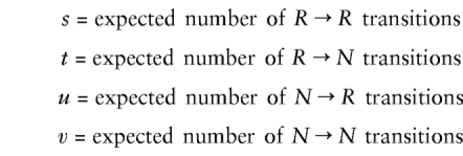where s+t+u+v=n, the total sample size. Then the likelihood is

which can be maximized analytically to give

Example

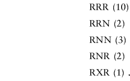
Consider the following simple 3-marker data set, with the number in parentheses indicating how many chromosomes with that observed pattern appear in the data set:

We start with the guess that y₁=y₂=.2.

E-step

There are eight possible true three-character strings: RRR, RRN, RNR, RNN, NNN, NNR, NRN, and NRR. We need to calculate the expected number of each of these strings, given the data set and the guessed parameter values. Each data string that does not include Xs or Us just contributes a value of one to the corresponding expected value. For example, each RRR string contributes a value of one to the expected number of true RRR strings, and contributes zero to all other counts. The one RXR string in the data set contributes some probability to the expected count of RRRs, and some probability to the expected count of RNRs. The probability that the RXR really represents RRR is

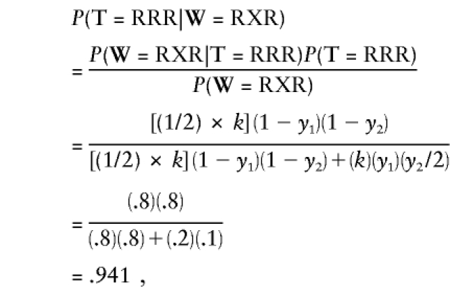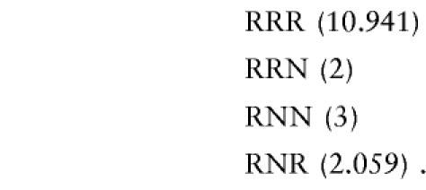
where k represents the previously discussed constants that drop out of the calculation. So the RXR string contributes .941 to the expected number of RRRs and 1-.941=.059 to the expected number of RNRs. The expected data set at this iteration is then

M-step

The likelihood of the expected data is

Maximized separately for the two intervals using equation (A1), this yields y₁=.281 and y₂=.249. These values can then be fed back into the E-step for the next iteration. The values for the full run with NDJMap are given in table A1.

Table A1.

Values of y₁ and y₂ over the Full Run of NDJMap

Iteration	y1	y2
1	.200	.200
2	.281	.249
3	.284	.253
4	.284	.253
5	.284	.253
6	.284	.253

References

- Baum LE, Petrie T, Soules G, Weiss G (1970) A maximization technique occurring in the statistical analysis of probabilistic functions of Markov chains. Ann Math Statist 41:164–171 [Google Scholar]
- Baum LE (1972) An inequality and associated maximization techniques in statistical estimation for probabilistic functions of Markov processes. Inequalities 3:1–8 [Google Scholar]
- Chakravarti and Slaugenhaupt (1987) Methods for studying recombination on chromosomes that undergo nondisjunction. Genomics 1:35–42 [DOI] [PubMed]
- Chakravarti A, Majumder PP, Slaugenhaupt SA, Deka R, Warren AC, Surti U, Ferrell RE, et al (1989) Gene-centromere mapping and the study of non-disjunction in autosomal trisomies and ovarian teratomas. Prog Clin Biol Res 311:45–79 [PubMed]
- Collins A, Teague J, Keats BJ, Morton NE (1996) Linkage map integration. Genomics 36:157–62 [DOI] [PubMed]
- Cote GB, Edwards JH (1975) Centrometric linkage in autosomal trisomies. Ann Hum Genet 39:51–59 [DOI] [PubMed]
- Deka R, Chakravarti A, Surti U, Hauselman E, Reefer J, Majumder PP, Ferrell RE (1990) Genetics and biology of human ovarian teratomas. II. Molecular analysis of origin of nondisjunction and gene-centromere mapping of chromosome I markers. Am J Hum Genet 47:644–655 [PMC free article] [PubMed]
- Halloran SL, Chakravarti A (1987) DSLINK: a computer program for gene-centromere linkage analysis in families with a trisomic offspring. Am J Hum Genet 41:350–355 [PMC free article] [PubMed]
- Koehler KE, Hawley RS, Sherman S, Hassold T (1996) Recombination and nondisjunction in humans and flies. Hum Mol Genet 5:1495–1504 [DOI] [PubMed]
- Lamb NE, Freeman SB, Savage-Austin A, Pettay D, Taft L, Hersey J, Gu Y, et al (1996) Non-disjunction of chromosome 21: evidence for initiation of all maternal errors during meiosis I. Nat Genet 14:400–405 [DOI] [PubMed]
- Little RJA, Rubin DB (1987) Statistical analysis with missing data. John Wiley & Sons, New York [Google Scholar]
- Mascari MJ, Ladda RL, Woodage T, Trent RJ, Lai LW, Erickson RP, Cassidy SB, et al (1993) Perturbed recombination of chromosome 15 in Prader-Willi patients with maternal disomy. Am J Hum Gen Suppl 53:A260 [Google Scholar]
- Meng X-L, Rubin DB (1991) Using EM to obtain asymptotic variance-covariance matrices: the SEM algorithm. J Am Stat Assoc 86:899–909 [Google Scholar]
- Morton NE, Andrews V (1989) MAP, an expert system for multiple pairwise linkage analysis. Ann Hum Genet 53:263–269 [DOI] [PubMed]
- Morton NE, MacLean CJ (1984) Multilocus recombination frequencies. Genet Res 44:99–108 [DOI] [PubMed]
- Morton NE, Keats BJ, Jacobs PA, Hassold T, Pettay D, Harvey J, Andrews V (1990) A centromere map of the X chromosome from trisomies of maternal origin. Ann Hum Genet 54:39–47 [DOI] [PubMed]
- Rabiner LR (1989) A tutorial on hidden Markov models and selected applications in speech recognition. Proc IEEE 77:257–285 [Google Scholar]
- Robinson WP, Bernasconi F, Mutirangura A, Ledbetter DH, Langlois S, Malcolm S, Morris MA, et al (1993) Nondisjunction of chromosome 15: origin and recombination. Am J Hum Genet 53:740–751 [PMC free article] [PubMed]
- Shahar S, Morton NE (1986) Origin of teratomas and twins. Hum Genet 74:215–218 [DOI] [PubMed]
- Sherman SL, Takaesu N, Freeman SB, Grantham M, Phillips C, Blackston RD, Jacobs PA, et al (1991) Trisomy 21: association between reduced recombination and non-disjunction. Am J Hum Genet 49:608–620 [PMC free article] [PubMed]
- Sherman SL, Petersen MB, Freeman SB, Hersey J, Pettay D, Taft L, Frantzen M, et al (1994) Non-disjunction of chromosome 21 in maternal meiosis I: evidence for a maternal age dependent mechanism involving reduced recombination. Hum Mol Genet 3:1529–1535 [DOI] [PubMed]
- Warren AC, Chakravarti A, Wong C, Slaugenhaupt SA, Halloran SL, Watkins PC, Metaxotou C, et al (1987) Evidence for reduced recombination on the non-disjoined chromosome 21 in Down syndrome. Science 237:652–654 [DOI] [PubMed]
- Zhao H, Speed TP (1998) Statistical analysis of half-tetrads. Genetics 150:473–485 [DOI] [PMC free article] [PubMed]