Linkage Analysis in the Presence of Errors IV: Joint Pseudomarker Analysis of Linkage and/or Linkage Disequilibrium on a Mixture of Pedigrees and Singletons When the Mode of Inheritance Cannot Be Accurately Specified

Abstract

There is a lot of confusion in the literature about the “differences” between “model-based” and “model-free” methods and about which approach is better suited for detection of the genes predisposing to complex multifactorial phenotypes. By starting from first principles, we demonstrate that the differences between the two approaches have more to do with study design than statistical analysis. When simple data structures are repeatedly ascertained, no assumptions about the genotype-phenotype relationship need to be made for the analysis to be powerful, since simple data structures admit only a small number of df. When more complicated and/or heterogeneous data structures are ascertained, however, the number of df in the underlying probability model is too large to have a powerful, truly “model-free” test. So-called “model-free” methods typically simplify the underlying probability model by implicitly assuming that, in some sense, all meioses connecting two affected individuals are informative for linkage with identical probability and that the affected individuals in a pedigree share as many disease-predisposing alleles as possible. By contrast, “model-based” methods add structure to the underlying parameter space by making assumptions about the genotype-phenotype relationship, making it possible to probabilistically assign disease-locus genotypes to all individuals in the data set on the basis of the observed phenotypes. In this study, we demonstrate the equivalence of these two approaches in a variety of situations and exploit this equivalence to develop more powerful and efficient likelihood-based analogues of “model-free” tests of linkage and/or linkage disequilibrium. Through the use of a “pseudomarker” locus to structure the space of observations, sib-pairs, triads, and singletons can be analyzed jointly, which will lead to tests that are more well-behaved, efficient, and powerful than traditional “model-free” tests such as the affected sib-pair, transmission/disequilibrium, haplotype relative risk, and case-control tests. Also described is an extension of this approach to large pedigrees, which, in practice, is equivalent to affected relative-pair analysis. The proposed methods are equally applicable to two-point and multipoint analysis (using complex-valued recombination fractions).

Introduction

There is a lot of rhetoric in the literature about whether one should apply “model-based” (e.g., Hodge and Elston ¹⁹⁹⁴; Greenberg et al. ¹⁹⁹⁶; Trembath et al. ¹⁹⁹⁷) or “model-free” (e.g., Farrall ¹⁹⁹⁷; Kruglyak ¹⁹⁹⁷) analysis methods to map the genes whose alleles predispose to complex disease. Most of the arguments, however, seem motivated more by philosophical dogma than practical and rational considerations—like the disagreement over the size and position of the flags on the negotiation table for the Panmunjom armistice talks (Joy 1955). Symmetries between “model-based” and “model-free” analysis methods have been recognized for many years (see Hyer et al. ¹⁹⁹¹; Knapp et al. ¹⁹⁹⁴; Kuokkanen et al. ¹⁹⁹⁶; Satsangi et al. ¹⁹⁹⁶; Whittemore ¹⁹⁹⁶; Trembath et al. ¹⁹⁹⁷; Terwilliger ¹⁹⁹⁸), yet the tension and confusion remain strong, with the field being somewhat polarized on this issue. We hope that the following comparative analysis of the underlying nature of “model-based” and “model-free” methods will help attenuate such contentious confusion.

In this study, we will start from first principles and derive the most common “model-free” statistics, and we will show that they are equivalent to “model-based” analysis under certain rather extreme assumptions about the mode of inheritance. Only when the same very simple data structure is sampled repeatedly from a population can truly “model-free” analysis be performed powerfully. In all other instances, some assumptions are required to reduce the df in the data to a manageable number. A model of genotype-phenotype correlation at a single trait locus is used in “model-based” analysis to infer disease-locus genotypes in a probabilistic manner, as a means of adding structure to the underlying probability model. “Model-free” analysis accomplishes this goal by other, more ad hoc approaches, such as assuming that all meioses have equal probability of being informative for linkage at the disease locus (i.e., disease-locus genotype D/+), with the disease-predisposing allele (D) being transmitted with equal probability from each D/+ parent to each affected offspring. Though one may hesitate to formally call these assumptions a “model” of the mode of inheritance, they often lead to test statistics which will be shown to be equivalent to “model-based” analysis under certain extreme assumptions about the mode of inheritance.

Another area of confusion which is dominated by rhetoric is the distinction between linkage and linkage disequilibrium (LD) analyses. In fact, both linkage and LD are correlations between genotypes of two loci (within and between pedigrees, respectively), not between the genotype of one (marker) locus and a phenotype influenced by genotypes of another (disease) locus. The ascertainment schemes have traditionally been quite different when linkage or LD is the focus of inference, with emphasis on ascertainment of unrelated affected and unaffected individuals (for LD analysis) and on pedigrees with as many affected relatives as possible (for linkage analysis). However, as has been argued repeatedly (e.g., Risch and Merikangas ¹⁹⁹⁶; Terwilliger and Göring in press), the power to detect LD increases when affected relatives are ascertained, since this will increase the probability that affected individuals have a multifactorial disease for (the same) genetic reason(s). Since, in most cases, investigators have a mixture of different data structures available—such as pedigrees, triads, and singletons—we propose that all of the data be analyzed jointly, using likelihood-ratio tests for linkage and/or LD. Joint analysis of linkage and LD on the totality of the available data has been advocated by others as well (Martin et al. 1997; Teng and Siegmund ¹⁹⁹⁷; Excoffier and Slatkin ¹⁹⁹⁸; Terwilliger and Weiss ¹⁹⁹⁸; Zhao et al. ¹⁹⁹⁸; Terwilliger and Göring in press). We demonstrate here that “model-free” likelihood-based analysis using “pseudomarker” genotypes is more powerful than the conventional “model-free” tests when both linkage and LD are present, and, unlike some conventional “model-free” statistics, remains powerful for detection of either of the two phenomena in the absence of the other.

Unified Theoretical Model of Likelihood-Based Linkage and LD Analysis

In both “model-based” and “model-free” analysis, inference can be made based on the likelihood, L∝P(Ph,G_M), where Ph represents the vector of observed disease phenotypes and G_M the vector of observed marker-locus genotypes (of one or multiple marker loci) for all individuals in the data set. This likelihood is then compared under different hypotheses, to test whether the underlying genotypes of the disease and marker loci are correlated (see Göring and Terwilliger ^2000c; Terwilliger and Göring in press). In “model-based” analysis, this likelihood is computed by partitioning over all possible underlying disease- and marker-locus genotypes for all individuals in the data set (g_D and g_M), as

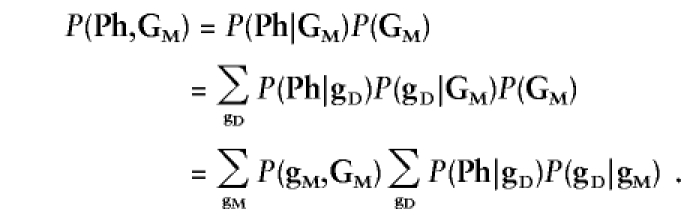In this formulation of the likelihood, P(g_M,G_M) is a function of the marker-locus genotype-frequency distributions (and genotyping-error rates), P(Ph|g_D) is a function of the assumed relationship between disease-locus genotypes and disease phenotypes, and P(g_D|g_M) is a function of linkage and/or LD between disease and marker loci, as well as disease-locus genotype frequencies, as enumerated in table 1 of Göring and Terwilliger (2000c). P(g_D|g_M) is the focus of inference in linkage and LD analysis, as it contains all the information about correlations among the loci. By contrast, in “model-free” analysis, the likelihood is expanded as L∝P(Ph,G_M)=P(G_M|Ph)P(Ph). In order to avoid stratifying over underlying disease- and marker-locus genotypes (which would require some “model” assumptions), the same simple data structure (i.e., a particular pedigree structure with a particular set of phenotypes, Ph) is repeatedly sampled from the population (e.g., affected sib-pairs, triads, singletons, etc.). In this situation, all possible outcomes G_M can be categorically enumerated such that the probability P(G_M|Ph) would follow a multinomial distribution (see below for examples). A primary drawback of conventional “model-free” methods is that they only behave in a straightforward and predictable manner when the same pedigree/phenotype structure can be ascertained multiple times from a population.

Table 1.

Mean, Variance, Skewness, and Kurtosis of the “All-Pairs” ASP Mean Test Statistic, ASP_AP, as a Function of Sibship Size^[Note]

No. of Affected Sibs	Mean	Variance	Skewness	Kurtosis
2	0	1	0.000	1.000
3	0	1	1.155	2.333
4	0	1	1.633	4.667
5	0	1	1.897	6.400
6	0	1	2.066	7.667
7	0	1	2.182	8.619
8	0	1	2.268	9.357
9	0	1	2.333	9.944
10	0	1	2.385	10.422
N(0,1)	0	1	0.000	3.000

Note.—The mean, variance, skewness, and kurtosis are computed based on IBD sharing from one parent in a single nuclear family of the indicated size, under the assumption of a fully informative marker locus. The moment coefficient of kurtosis given here is computed as (note that some statisticians prefer using a different measure of kurtosis, in which 3 is subtracted from the quantity given here).

In “model-based” analysis, the question of inferential focus is whether the disease- and marker-locus genotypes are correlated; that is, whether P(g_D|g_M)=P(g_D), independent of g_M. Such correlation could be due to linkage, LD, or both, and it can be parameterized as a function of both phenomena, no matter what data structures have been ascertained (Göring and Terwilliger ^2000c; Terwilliger and Göring in press). In “model-free” analysis, the analogous question is whether the observed marker-locus genotypes are independent of the observed disease phenotypes; that is, whether P(G_M|Ph)=P(G_M), independent of Ph. If this probability is partitioned over the underlying marker- and disease-locus genotypes, one obtains , where only the term P(g_M|g_D) is a function of linkage and/or LD. Thus one can see that, fundamentally, “model-free” inference is likewise focused on whether the underlying marker- and disease-locus genotypes are correlated; that is, whether P(g_M,g_D)=P(g_M)P(g_D) in both cases. The difference between the two approaches relates to the assumptions one needs to make about g_D. By repeated ascertainment of the same simple data structure, no such assumptions are required in “model-free” methods. Such ascertainment minimizes the number of parameters required to express the general likelihood as a multinomial function of the enumerated set of all possible observations G_M. In order to perform a “model-free” analysis on larger data structures (or even a variety of small ones), some simplifying assumptions are required to structure the space of possible outcomes G_M as a function of the parameters of inferential interest.

To this end, we propose structuring the correlations between Ph and G_M in a “model-free” manner, by assigning “genotypes” of an artificial “pseudomarker” locus, g_P, to all individuals in the data set as a surrogate for the observed set of disease phenotypes, Ph. This leads to statistical tests based on the likelihood L∝P(g_P,G_M)=P(G_M|g_P)P(g_P). P(g_P) can be absorbed in the constant of proportionality, because it is constant under all hypotheses, since the pseudomarker genotypes are assigned solely on the basis of the observed phenotype structure. We do not intend to imply that there is a unique way that pseudomarker genotypes must be assigned in practice, though we will focus on simple algorithms that lead to statistical tests analogous to many of the traditional “model-free” methods, as shown below. According to these algorithms, pseudomarker genotypes would be assigned in such a way as to make informative for linkage those meioses connecting affected individuals, so that the affected individuals inherit as many pseudomarker alleles identical by descent (IBD) as possible. In nuclear pedigrees, this can be accomplished by making both parents informative for linkage (e.g., pseudomarker genotype D/+), irrespective of their phenotype, with each of their affected children receiving the parental D alleles. Since most “model-free” analyses are conducted in an “affecteds-only” manner (because it is hypothesized that the “unaffected” phenotype is not a reliable predictor of the underlying disease-locus genotype for a complex disease), all remaining individuals would have unknown pseudomarker genotype. If one wished to contrast affected and unaffected individuals in the analysis as well, such as in discordant sib-pair analysis, one could assume that the unaffected sibs received the parental + allele, rather than the D allele transmitted to the affected sibs. Singleton individuals and larger pedigrees can be assigned pseudomarker genotypes in an analogous manner. Applying this algorithm to singletons and nuclear pedigrees of various size yields likelihood-ratio tests of linkage and/or LD that are equivalent to the sib-pair mean test, the transmission/disequilibrium test (TDT), the haplotype-based haplotype relative risk (HHRR) test, and traditional case-control analyses. In addition, such application leads to novel and more general “model-free” tests that can be applied to a mixture of data structures and can allow for joint testing of linkage and LD. Other models for phenotype→pseudomarker genotype transformation in general pedigrees are discussed below.

In “model-based” analysis, as was described above, the likelihood of the observed disease phenotypes, Ph, and marker-locus genotypes, G_M, is partitioned over all possible disease-locus genotype vectors, g_D, for all individuals in the data set, weighted by their prior probabilities. One may describe this procedure as a probabilistic assignment of disease-locus genotypes, in contrast to a deterministic pseudomarker algorithm. For a given pedigree structure and observed disease phenotypes, the number of possible disease-locus genotype vectors depends on the assumed disease model. If one allows for phenocopies—that is, P(affected|+/+)>0—and incomplete penetrance—that is, P(affected|D/D)<1—then every disease-locus genotype (D/D, D/+, +/+) would be admissible for every individual in every data set (though not all combinations of genotypes would be possible, because of Mendel's laws [Mendel ¹⁸⁶⁶]), such that the likelihood would have to be computed over a large number of underlying disease-locus genotype vectors, g_D. For a model assuming full penetrance and no phenocopies, however, the number of disease-locus genotype vectors will be much smaller, and sometimes just a single vector, g_D, may be admissible. Notice that such an analysis is similar to pseudomarker analysis, in which disease-locus genotypes are assigned deterministically on the basis of the observed phenotypes. In this sense, the stronger the genotype-phenotype correlation assumed in a “model-based” analysis, the closer it becomes, paradoxically, to “model-free” analysis!

The set of inferred disease-locus genotypes, g_D (or, analogously, g_P in pseudomarker analysis), generally will not be identical to the true genotypes of the disease locus. As is generally the case in likelihood analysis, errors will often lead to biased estimates of underlying parameters. In linkage analysis, the parameter of interest—the estimate of which will be biased—is the recombination fraction, θ, as follows. Some proportion, α, of meioses that are truly informative for linkage (i.e., parental genotype is D/+) will be correctly inferred to be informative, and some proportion, β, of meioses that are actually uninformative for linkage (i.e., parental genotype is either D/D or +/+) will be incorrectly inferred to be informative, according to the probability model shown in figure 1. If a meiosis were misclassified as uninformative, linkage information would be discarded inappropriately (i.e., the signal would be reduced), but no bias in the estimate of θ would result. However, if a meiosis were misclassified as informative, it would be inappropriately inferred to be recombinant 50% of the time (i.e., noise would be added into the analysis), resulting in an upward bias in the estimate of θ. Both types of error can lead to reduction of power. If the number of meioses which are actually informative for linkage (D/+) is K_I and the number of meioses which are actually uninformative for linkage is K_U, the expected maximum-likelihood estimate of θ (assuming absence of misclassification errors in the recombination status of the truly informative meioses—see Göring and Terwilliger ^{2000a, 2000b}) would be . In pseudomarker analysis, every meiosis is assumed to be informative, and, accordingly, α=1 and β=1, and , which is biased upward unless K_U=0 or θ=0.5. Such inflation of the estimate of θ can be allowed for in an analysis through the use of complex-valued recombination fractions, as described by Göring and Terwilliger (2000a, 2000b).

Figure 1.

Observed recombination status as a function of meiotic informativeness. In reality, every meiosis is either informative (I) or uninformative (U) for linkage. A meiosis is only informative when a parent is heterozygous at both the disease locus (D/+) and the marker locus. Sometimes, however, the parental disease-locus genotypes will be misspecified by the algorithm used to assign disease-locus genotypes (such as the proposed pseudomarker algorithms), which is part of the analysis. This will lead either to an informative meiosis being misclassified as uninformative (with probability 1−α) or to an uninformative meiosis being misclassified as informative (with probability β). Meioses classified as uninformative are censored from the analysis. Among those meioses classified as informative, the truly informative ones will show recombination with probability θ, whereas the ones which are in reality uninformative will show recombination with probability .5. This often leads to an upward bias in the estimate of θ, the expectation of which is given by , which is >θ unless θ=.5, β=0 or K_U=0, where K_I and K_U are the number of truly informative and uninformative meioses, respectively. In (recessive) pseudomarker analysis, α=1 and β=1, and thus , which is >θ unless θ=.5 or K_U=0. The bias in the estimate of θ can be accounted for through the use of complex-valued recombination fractions (Göring and Terwilliger ^2000a). For further development of this model, see Terwilliger and Göring (in press).

Common “Model-Free” Methods and Their Pseudomarker Analogues

Linkage Tests Based on Affected Sib-Pairs

A common ascertainment scheme for “model-free” linkage analysis is to collect a large sample of affected sib-pairs, without regard to the parental phenotypes (see Penrose 1935). In this scheme, Ph would be “in a nuclear family with two sibs, both sibs are affected with the disease,” and GM would represent the observed marker-locus genotypes of both sibs and their parents. If parents are not available for genotyping, one can sum over all their admissible marker-locus genotypes, weighted by P(GM|gM) as described above. On this data structure, one can categorize the possible outcomes, GM, as a function of how many alleles the two sibs share IBD (0, 1, or 2), with corresponding multinomial likelihood L∝pX00pX11(1-p0-p1)X2, where pi is the probability with which a sib-pair shares i alleles IBD, and Xi is the number of sib-pairs in the data set which are observed to share i alleles IBD. Under the null hypothesis that marker- and disease-locus genotypes are uncorrelated (i.e., there is no linkage between the loci), p0=0.25, and p1=0.5. Under the alternative hypothesis of linkage, the likelihood would be maximized over all possible values for these parameters (sometimes restricted to a portion of the total admissible parameter space—see Holmans 1993), leading to a likelihood-ratio test of the form

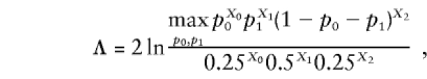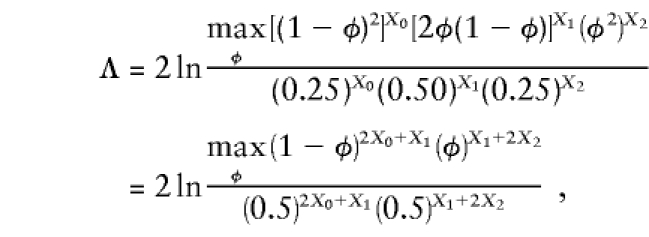
which is asymptotically distributed according to χ² distribution with 2 df, when the p_i are unconstrained (see Blackwelder and Elston ¹⁹⁸⁵; Holmans ¹⁹⁹³). If one assumes (as in the affected sib-pair mean test) that the transmission of marker-locus alleles from the two parents is independent, conditional on the observed phenotypes, one of those df can be eliminated. If we define φ=P (two affected sibs share an allele IBD from a given parent), then p₀=(1-φ)², p₁=2φ(1-φ), and p₂=φ². When such structure is added to the underlying probability space, the likelihood-ratio test of linkage, Λ, can be rewritten as

which is asymptotically distributed as a 50-50 mixture of point-mass at 0 and χ² distribution with 1 df (Nordheim 1984; Tai and Chen ¹⁹⁸⁹).

In a pseudomarker linkage analysis, under the assumption that all meioses connecting affected individuals are informative for linkage, both parents of an affected sib-pair would be assigned pseudomarker genotype D/+, and, assuming that the affected sibs share as many pseudomarker alleles IBD as possible, the pseudomarker genotypes of the affected sibs would be set to D/D, as illustrated in figure 2. In this model, the probability that two sibs inherit the same marker-locus allele IBD from a single parent would be φ=θ²+(1-θ)², and the likelihood-ratio test of linkage comparing G_M and g_P can be shown to be equal to

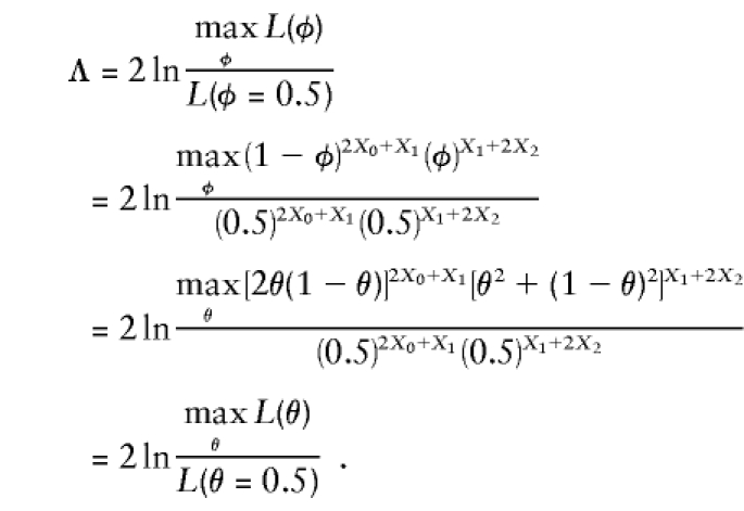Since either parameterization gives an equivalent coverage of the admissible probability space, the equivalence of both approaches in the two-point case is established (see also Knapp et al. ¹⁹⁹⁴; Kuokkanen et al. ¹⁹⁹⁷; Satsangi et al. ¹⁹⁹⁷; Trembath et al. ¹⁹⁹⁷; Terwilliger ¹⁹⁹⁸). To establish equivalence in the multipoint case, one needs to use complex-valued recombination fractions, which we have introduced elsewhere (Göring and Terwilliger ^2000a). Briefly, a complex-valued recombination fraction, Θ=θ+εi, consists of two components: θ (the probability of actual recombination between alleles of disease and marker loci) and ε (the probability of apparent recombination events caused by errors in the assignment of disease-locus genotypes). Though these two components cannot be separated in two-point linkage analysis, they are identifiable in multipoint analysis. In Göring and Terwilliger (2000a), the equivalence of two-point analysis and multipoint analysis using complex-valued recombination fractions has been established by arbitrarily fixing θ=0 between the disease locus and some position, x_D, on the chromosome. The alternative-hypothesis likelihood is maximized over ε, and compared to the null hypothesis likelihood in which ε=0.5, such that the multipoint pseudomarker likelihood-ratio statistic, on a set of affected sib-pairs, would be

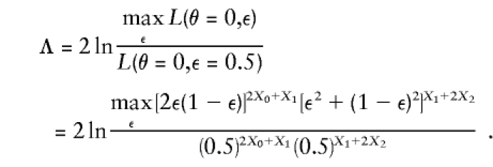This multipoint statistic has the same distribution as the two-point statistic (though, when maximized over map position, a correction for multiple testing is necessary as in any multipoint analysis—see Dupuis et al. ¹⁹⁹⁵). The equivalence of the pseudomarker test (with complex-valued recombination fractions) and the affected sib-pair mean test is thus established for the multipoint situation as well.

Figure 2.

Pseudomarker genotype assignment on a nuclear pedigree. The pseudomarker genotypes are shown as assigned in the pseudomarker analogue of the affected sib-pair mean test. The unaffected sibs would be assigned genotype +/+ instead of ?/? in discordant sib-pair analysis. The same genotype assignment rule is also used in other pseudomarker-based analyses on nuclear pedigrees and triads (see text for details on pseudomarker genotype assignment schemes for other data structures).

Linkage Analysis on Larger Sibships

The conventional sib-pair analysis methods and their pseudomarker analogs presented above are completely equivalent only when the data set consists solely of nuclear pedigrees with exactly two affected sibs. In practice, investigators typically also ascertain larger sibships, with more than two affected sibs, since under most plausible genetic models of disease it is more likely that disease alleles of strong effect are segregating in a sibship ascertained through presence of three affected individuals than in a sibship ascertained through presence of only two affected individuals, and so on (see Lathrop et al ¹⁹⁹⁶; Terwilliger and Göring in press). A corollary of this is that an affected sib-pair selected from a sibship ascertained through the presence of more than two affecteds will be more likely to share disease alleles IBD than an affected sib-pair with no additional affected siblings. For this reason, it is desirable to have sibships with as many affected individuals as possible. The problem is that the simple “pairs-based” analysis methods cannot be applied in a straightforward manner. Blackwelder and Elston (1985) analyzed the statistical properties of a simpler algebraic representation of the mean test,

which they showed to be asymptotically distributed as a N(0,1) random variable under the hypothesis of no linkage, even if one breaks a sibship of size s into all s(s-1)/2 possible sib-pairs and applies this statistical test as if they were all independent (in which case we denote it as ASP_AP). They showed that the mean and variance of this ASP_AP statistic indeed remain 0 and 1, respectively. However, the skewness and kurtosis of the distribution of this statistic can deviate dramatically from the values expected for a N(0,1) variable, as shown in table 1 for allele sharing from a single parent in a single sibship. This can lead to a high rate of false-positive linkage findings, even in fairly large data sets, as shown below by simulation, though the problem goes away asymptotically (i.e., if one had an infinitely large data set) according to the central limit theorem (de Moivre ¹⁷⁵⁶). Based on power considerations, Suarez and Hodge (1979) proposed a weighting function to treat a sibship of size s as being equivalent to (s-1) independent sib-pairs (ASP_WP). While this approximate solution attenuates the effect of a small number of large sibships, it still leads to substantial skewness and kurtosis relative to the assumed N(0,1) distribution and, thus, a risk of false-positive results (see simulation results below).

Pseudomarker analysis, however, allows larger sibships to be analyzed by a straightforward extension, by simply assigning pseudomarker genotype D/D to all affected sibs in each sibship. This procedure leaves the distribution of the LOD-score statistic invariant (see simulation results below), though one can no longer write the LOD score as a function of X₀, X₁, and X₂, but rather as a function of the entire vector G_M. Unaffected siblings can be included in pseudomarker analysis by either of two approaches. If one wanted to preserve the “affecteds-only” nature of the analysis, one should leave the pseudomarker genotype indeterminate for unaffected sibs (i.e., they would only be used to help infer unknown parental marker-locus genotypes and to infer phase in multipoint analysis). If one wanted to do a discordant sib-pair analysis, the unaffecteds could be assigned pseudomarker genotype +/+, resulting in a test that is equivalent to the discordant sib-pair mean test (S.A.G.E. ¹⁹⁹⁴).

LD Analysis on Singletons (Case-Control Studies)

The simplest experimental design for LD analysis involves random ascertainment of a large sample of unrelated individuals with the disease (cases) and without the disease (controls). In the absence of LD, one expects the distribution of genotype frequencies to be identical in cases and controls, assuming the samples were ascertained in an unbiased manner from the same genetic population. In “model-free” analysis of LD, one wants to know whether P(G_M|Ph)=P(G_M), independent of Ph, which is the same abstract hypothesis tested in “model-free” linkage analysis. However, since the sample consists solely of unrelated individuals, there is no way to look at segregation of alleles in pedigrees, and the correlations which might exist between marker-locus genotypes and disease phenotypes are a function of LD rather than linkage. Note that we use the term “LD” to refer to any gametic phase disequilibrium that may exist between alleles of disease and marker loci, irrespective of cause.

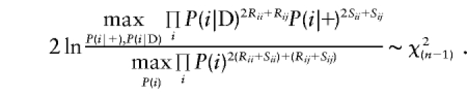
In traditional case-control analysis, one tests for correlations by comparing the genotype-frequency distribution in cases and controls; that is, testing whether P(G_M|case)=P(G_M|control). For simplicity, let us restrict ourselves to consideration of a single-marker locus (though this can be directly generalized to the multipoint case), with parameters as follows: r_ij=P(genotype ij|case), s_ij=P(genotype ij|control), and R_ij and S_ij represent the number of cases and controls, respectively, with genotype ij. A likelihood-ratio test of LD between alleles of the disease locus and a marker locus with n alleles could be formulated as

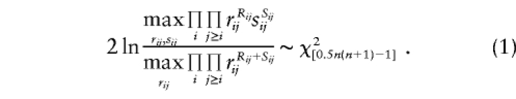It should be noted that this test is analogous to a traditional contingency-table χ² test (with continuity correction) of LD, comparing genotype frequencies in cases and controls. To reduce the number of df in the analysis, one often assumes the existence of Hardy-Weinberg equilibrium (HWE) in both case and control samples. If we define the allele frequencies of allele i in cases and controls as g_i and h_i, respectively, then the assumption of HWE implies that r_ij=2g_ig_j when i≠j, and r_ii=g²_i. Adding this structure to the probability model leads to a likelihood-ratio test statistic that reduces the number of df in the analysis by n(n-1)/2

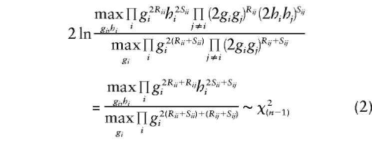This test is analogous to the conventional contingency-table χ² test (with continuity correction) (Wilks 1935) comparing allele frequencies in cases and controls. It should be noted that the assumption of HWE is reasonable under the null hypothesis, making the test valid, but that this is not formally possible under the alternative hypothesis, since, in the presence of LD, HWE cannot hold in both cases and controls individually if it holds in the population as a whole (see Terwilliger and Göring in press), though this model serves as a reasonable first-order approximation. One could allow for a more realistic parameterization by allowing the inbreeding coefficient, F_is, to admit nonzero values, which may differ between cases and controls, as described elsewhere [i.e. r_ij=(1-F_is)2g_ig_j if i≠j; r_ii=(1-F_is)g²_i+g_iF_is] (see Hartl and Clark ¹⁹⁹⁷; Agarwala et al. ¹⁹⁹⁹; Hovatta et al. ¹⁹⁹⁹; Göring and Terwilliger ^2000c).

A test equivalent to (2) can be derived using our pseudomarker strategy. Inference in case-control analysis is based on the allele frequencies of the marker locus conditional on the phenotype. If one were to assign pseudomarker genotype D/D to all cases and pseudomarker genotype +/+ to the controls, by analogy to discordant sib-pair analysis, as described above, the likelihood could be written as a function of the haplotype frequencies P(Di)=P(i|D)P(D) and P(+i)=P(i|+)P(+). A likelihood-ratio test comparing the allele frequency distributions in cases and controls, using this pseudomarker strategy, could be written as follows (after canceling out the P(D) and P(+) terms from both numerator and denominator)

This test is stochastically equivalent to (2), replacing parameters g_i by P(i|D), etc., which have the same parameter space. Therefore, the pseudomarker LD test and the conventional “model-free” contingency-table χ² test are shown to behave identically. Note that one could allow for nonzero values for F_is, the inbreeding coefficient, in pseudomarker analysis, as above. For purposes of generality, the pseudomarker likelihood-ratio test of LD will be written as , where δ_D is used as a shorthand notation for the LD between the alleles of the disease and marker loci, as in Göring and Terwilliger (2000c). This notation is not intended to imply any specific parametric model of LD, though one can impose restrictions, as desired, to further minimize the number of df in the analysis.

If one wanted to do such a pseudomarker analysis of LD using the ILINK program (Lathrop et al. 1984), one would have to create artificial “pedigrees” from the singleton cases and control individuals. A simple way to do this in practice is to create pedigrees in which a pair of genotyped cases and/or controls are the parents of a hypothetical child with unknown genotypes at both loci (e.g., Annunen et al. ¹⁹⁹⁹; Kainulainen et al. ¹⁹⁹⁹). In this way, both cases and controls would be assumed to be unrelated pedigree founders by the software, and the likelihoods would be proportional to those described above. Analogous likelihood-ratio test statistics can be computed in a “model-based” manner, as implemented in the EH program (see Terwilliger and Ott ¹⁹⁹⁴, section 24.2), or by creation of these artificial “pedigrees” from a case-control sample and estimation of haplotype frequencies conditional on the disease-allele frequency and mode of inheritance with ILINK, with the conditional haplotype frequency model recently implemented as of version 4.1P of the FASTLINK software package (Cottingham et al. 1993).

LD Analysis on Triads (HHRR Tests) and Sibships

It is often advisable to ascertain the parents of an affected individual as well, especially when multiple marker loci are being analyzed jointly, as this can allow more accurate prediction of the phase of the marker-locus alleles (see Hodge et al. ¹⁹⁹⁹). Rubinstein et al. (1981) proposed such an ascertainment scheme, on the basis of sampling affected individuals grouped with their parents in “triads” to circumvent other problems arising from population stratification, suggesting that the alleles “not transmitted” by the parents to the affected offspring could serve as a control sample. Assuming HWE, Ott (1989) demonstrated that the nontransmitted parental alleles are an unbiased sample of alleles from the population, such that the probability model described above for case-control samples can be applied directly to the transmitted and nontransmitted genotypes in such triads as well. As above, R_ij would be the number of affected individuals with genotype ij, while S_ij would now represent the number of triads with nontransmitted parental alleles i and j (i.e., one parent with allele i not transmitted to the affected child and one with j not transmitted). In the original formulation of the haplotype relative risk, inference was based on a comparison of such “genotype” frequencies (GHRR), analogous to (1) above (Falk and Rubinstein 1987). Terwilliger and Ott (1992) proposed a reduction of the number of df in the underlying probability model (HHRR) by assuming that HWE holds in both samples of transmitted and nontransmitted genotypes alike, leading to statistical tests of the form of (2) above. They demonstrated that this is more powerful in a wide variety of situations, as expected, because of the reduction in the number of df.

Terwilliger and Ott (1992) also considered tests on this data structure which were restricted to parents who are heterozygous at the marker locus, to test whether they transmitted allele i or j to their affected offspring with equal probability; that is, whether

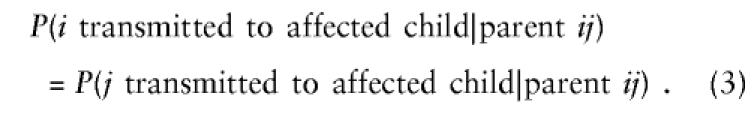They proposed testing this hypothesis using a McNemar (1947) paired sampling test, and demonstrated that this approach, as a test of LD, was less powerful than the HHRR test. Even though the assumption of HWE was necessary to demonstrate the independence of the transmitted and nontransmitted allele-frequency distributions, the McNemar test does not make this assumption, leading to slightly reduced power when HWE applies. When HWE does not hold, the HHRR test tends to be conservative, and only when the deviation from HWE is unrealistically large can the McNemar test exceed the HHRR in power.

In the ascertained triads, the affected individuals have the same disease- and marker-locus allele-frequency distribution as the affected individuals in case-control analysis, since parental phenotypes are not part of the ascertainment scheme. In pseudomarker analysis, it is therefore logically consistent to assign pseudomarker genotype D/D to the affected offspring in triads, as we did to the affected singletons in case-control pseudomarker analysis. Since one wishes to contrast the transmitted and nontransmitted alleles of the parents, the parents should be assigned pseudomarker genotype D/+. Under the momentary assumption that θ=0 between disease and marker loci, the likelihood of a triad with an affected child with genotype ij and parents with nontransmitted alleles k and l would be L∝P(i|D)P(j|D)P(k|+)P(l|+). Note that in case-control analysis, if one had an affected individual with genotype ij and a control individual with genotype kl, L∝g_ig_jh_kh_l, which is analogous. The resulting test statistics, which are both of the form of (2), would thus be stochastically equivalent.

If θ is significantly larger than 0, there is unlikely to be meaningful allelic association, period (see Terwilliger and Weiss ¹⁹⁹⁸). When one allows for LD, however, the likelihood of a triad is a function of θ as well, and, when θ=0.5, the HHRR will not be able to detect any allelic association that may exist—caused, for example, by population stratification (Chase 1977; Ott ¹⁹⁸⁹). For this reason, many investigators choose this ascertainment scheme as a means of distinguishing LD caused by linkage from correlations resulting from poor sampling, or other phenomena which may lead to nonindependence of the allele frequencies of unlinked loci (see Hovatta et al. ¹⁹⁹⁹). If one uses ILINK to maximize the likelihood, assuming such pseudomarker genotypes, the test statistic could be computed either by fixing θ to 0, or by computing the profile likelihood maximized over θ, which leads to an equivalent statistical test when only independent triads are analyzed, and a more reasonable one when larger pedigrees are included (see below). The resulting test statistic for LD allowing for linkage would be (notice that we used the same symbol above for the statistic on case-control data, because the likelihood of such data is not a function of θ, and both expressions are therefore equivalent for case-control data). As in Göring and Terwilliger (2000c), in the case of multipoint analysis, the symbol θ can be generalized to the map position of the disease-locus (x_D) relative to those of the marker loci (x_i). To extend this pseudomarker analysis to nuclear pedigrees with multiple affected sibs, one would simply assign the latter pseudomarker genotype D/D, keeping the parental genotypes as D/+, in which case Ψ can be computed on the larger sibships as well.

This test statistic is expected to asymptotically have a χ²₍₁₎ distribution under the null hypothesis of no LD when the marker locus is diallelic. Note that, in HHRR parlance, the two-sided nature of the test means that it is not known which of the two marker-locus alleles is associated with the D allele. When there are n alleles, the distribution should asymptotically converge to χ²_(n-1). This statistic, while equivalent to the HHRR in the case of singleton affecteds, allows inclusion of multiple affected siblings in the analysis of LD, rather than the usual approach of selecting one individual per family for association analysis, thus enabling a more efficient use of all the data. Of course, one could add further structure to the haplotype frequency space to reduce the number of df in the analysis of a multiallelic marker locus, for example, by using the likelihood model of Terwilliger (1995).

LD-Based Linkage Analysis in Larger Sibships (TDT) and Joint Tests of Linkage and LD

Spielman et al. (1993) noticed, in the framework of the McNemar paired sampling test proposed by Terwilliger and Ott (1992) for analysis of triad data, that the null-hypothesis condition in (3) is obtained either if there is no LD or if there is no linkage. Tests of this null hypothesis on triad data are therefore valid tests of either linkage equilibrium or the absence of linkage. Spielman et al. further noticed that equality of (3) also holds, in the absence of linkage, when multiple affected individuals in a larger family are included in the analysis as if they were independent, leading them to propose doing exactly that, which they called the transmission-disequilibrium test, or TDT. In the case of independent triads, (3) is an equality when there is either no LD or no linkage, but in larger pedigrees, (3) is an equality only under the hypothesis of no linkage; that is, if there is linkage but no LD, (3) is an inequality. To avoid confusion, we will distinguish between the tests based on the ascertainment conditions, such that whenever more than one affected individual per family is included, we will refer to the resulting statistical test as the TDT, and when only triads are used, we will refer to it as a McNemar test (to highlight that the latter is also a valid test of the null hypothesis of absence of LD).

One can assign pseudomarker genotypes as for the HHRR analysis above and compute profile likelihoods over the haplotype frequencies while focusing the inference on θ, as . This is analogous to the pseudomarker equivalent of affected sib-pair analysis, with LD as a nuisance parameter. On triad data with a diallelic marker locus, ζ would be numerically identical to , because there is only one df in such data. However, when the number of marker-locus alleles increases, the properties of these two statistics can become different. The same is true when there are multiple affected individuals in the same sibship, because they share alleles because of linkage, while having similar genotypes to affected individuals in other sibships because of LD.

The distribution of ζ can be a source of complication, as it depends on numerous factors, including the size and structure of the sample and the number of alleles of the marker locus. In general, it is most logical to first test for linkage independent of LD (Λ), following up a significant finding subsequently with a test of LD allowing for linkage (Ψ). A joint test for both linkage and LD would be of the form of

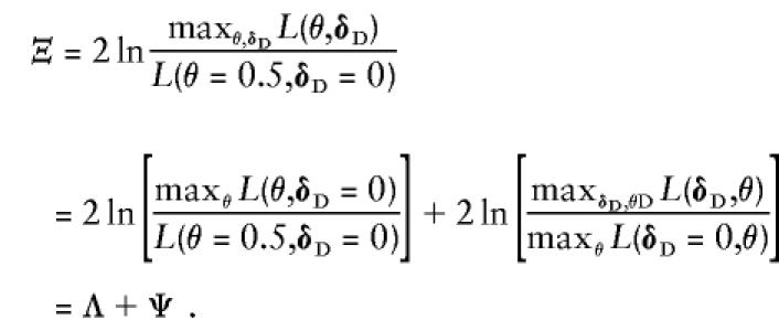This can only be significant if at least one of the component test statistics is significant individually. In general, we suggest testing for linkage first. Of course, it is difficult to interpret Ψ if there is no prior evidence of linkage (i.e., Λ is not significant), in which case the joint test, Ξ, should be applied instead. One can also obtain Ξ by reversing the order in which the hypotheses are tested, as

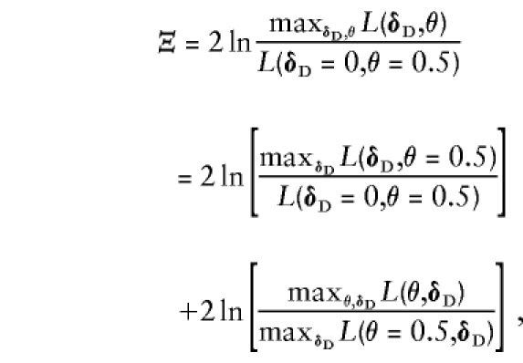where the latter term in the sum is ζ. If one has a sample that contains a large number of singleton cases and controls, one can obtain significant results in the first test (which would be asymptotically distributed as χ²_(n-1)). If that is the case, it makes sense to apply ζ to test for linkage allowing for the observed LD with profile likelihoods. In other situations, it can be dangerous to apply the test ζ. If one has a large and heterogeneous data set, including singleton case-control samples and families, then, asymptotically, the joint statistic Ξ would be distributed as a 50-50 mixture of χ²_(n-1) and χ²_(n). This assumption is generally conservative. The distribution of Ξ would be χ²_(n-1) on singleton-only (or triad-only) data, as there would be no linkage parameter in the likelihood formulation under either null or alternative hypotheses. If both triads and singletons exist, or if sibships are included, then the mixture distribution would be required, as the linkage parameter would exist in the data set.

Joint Analysis of Sibships, Triads, and Singletons

The three data structures most commonly ascertained in the study of complex diseases of late age of onset—nuclear pedigrees, triads, and singleton individuals—can be combined in one likelihood analysis by use of this pseudomarker algorithm (or, for that matter, conventional “model-based” analysis methods—Göring and Terwilliger ^2000c; Terwilliger and Göring in press). By analyzing all available data jointly, a more powerful and efficient set of statistics can be computed, instead of the conventional approach of analyzing each data structure independently. For “model-based” analysis, this has earlier been proposed (Terwilliger and Ott 1992; Terwilliger and Ott ¹⁹⁹⁴) and applied (Hellsten et al. 1993; Tienari et al. ¹⁹⁹⁴; Annunen et al. ¹⁹⁹⁹), and with the implementation of conditional haplotype frequency estimation in version 4.1P of FASTLINK (Cottingham et al. 1993) this technique is accessible to all. Using the pseudomarker approach, this can be done for “model-free” analysis as well (Kainulainen et al. 1999).

One should note that joint analysis of linkage and LD on pedigrees with untyped founders can be much more than the sum of the parts, as can be seen elsewhere (Hellsten et al. 1993; Tienari et al. ¹⁹⁹⁴; Annunen et al. ¹⁹⁹⁹; Kainulainen et al. ¹⁹⁹⁹). In the absence of LD, the possible phases of marker- and disease-locus alleles have equal prior probabilities. However, if there is LD, the prior probabilities of the two phases are not equal, leading to an increase in the effective number of “equivalent meioses” (Edwards 1976). If the founders are not genotyped, then the marker-locus genotype probabilities for all untyped individuals must also be estimated, together with the phase. Assuming absence of LD, this would be done independent of the disease. However, in the presence of LD, there is information about the marker-locus genotypes as well as the phase, which can be inferred from the disease-locus genotypes. Thus, not only the phase information is added, but also information about the marker-locus genotypes themselves. As a result, in the analysis of Hellsten et al. (1993), the LOD scores jumped from 9.55 to 30.93 when LD was allowed for in their parametric linkage analysis of a rare, autosomal recessive disease, with no increase in df. (In that analysis, however, haplotype frequencies were estimated from an independent data set.) In a joint pseudomarker analysis of sib-pairs without parents and independent case-control samples, multipoint LOD scores increased from 2.9 to 5.1 when LD was allowed for as a nuisance parameter (Kainulainen et al. 1999). (In that analysis, there was significant evidence of LD independent of linkage because of the large number of singleton cases and controls included in the analysis.)

Pseudomarker Methods Allowing for Dominance and Multigenerational Pedigrees

We have described a simple method of assigning pseudomarker genotypes on nuclear pedigrees and singleton individuals, leading to likelihood-ratio tests that are equivalent to many of the traditional, pairs-based, “model-free” methods. Of course, there are multiple ways one could assign such pseudomarker genotypes in pedigrees. A common practice in “model-based” linkage analysis is to analyze the data with both a “dominant” and a “recessive” single-locus model. There is no reason not to apply an analogous philosophy in pseudomarker analysis. One could assign pseudomarker genotype D/+ to all the affected individuals, and D/+ to one parent and +/+ to the other. If the parents are not genotyped (as was the case in the nuclear pedigrees of Kainulainen et al. ¹⁹⁹⁹), then it makes no difference which of the two parents is assumed to be informative for linkage at the pseudomarker locus. If they are both genotyped, however, there are two possible ways to proceed. If exactly one parent was affected with the disease, one could assign pseudomarker genotype D/+ to the affected parent and +/+ to the healthy one. However, if both parents have the same (or unknown) phenotype, then one should allow for both possible ordered parental-genotype combinations, such that the likelihood of a given pedigree would be L=0.5L(♂_D/+,♀_+/+) + 0.5L(♂_+/+,♀_D/+), where L(♂_D/+,♀_+/+) refers to the likelihood of a pedigree assuming the father is D/+ and the mother is +/+.

The larger and more complicated a pedigree is, the wider the variety of options that exist for pseudomarker genotype assignment, which is consistent with the increasing complexity of the possible correlations between Ph and G_M as the number of possible outcomes G_M increases. As pedigrees become larger and more complicated, the sensitivity of any linkage and/or LD analysis to the mode-of-inheritance assumptions of the disease grows exponentially, such that it may be important—and valuable—to try a wider variety of models on such pedigrees in both “model-based” and “model-free” analysis alike. Although it may sound paradoxical to speak of “models” in “model-free” analysis, the models are just different ways to add structure to the probability space in the presence of so many possible outcomes G_M. This is, in fact, exactly what people are doing when they analyze their data with several different “model-free” approaches, each of which makes slightly different simplifying assumptions about the underlying correlations between G_M and Ph.

To demonstrate how “dominant” pseudomarker genotypes could be assigned in general pedigrees (see Trembath et al. ¹⁹⁹⁷; Terwilliger ¹⁹⁹⁸), let us convert the conventional representation of a pedigree (e.g., figure 3A) into a graph (see Hartsfield and Ringel ¹⁹⁹⁴) with edges connecting parents to each of their children, such that each edge represents a meiosis in the pedigree (e.g., figure 3B). Let us denote a path connecting two individuals in the direction “child→parent→grandparent→…” as an “ascending” path and a path connecting two individuals in the opposite direction as a “descending” path, such that two individuals would be blood relatives if and only if they can be connected by a single ascending path, a single descending path, or a combination of one ascending path followed by one descending path through the pedigree. In a pedigree without loops, if all the affected individuals can be connected to a common ancestor using ascending paths alone, the affecteds and all individuals along these ascending paths to their nearest common ancestor would be assigned pseudomarker genotype D/+, irrespective of their phenotype, with their spouses being assigned pseudomarker genotype +/+. The only exception would be the nearest-common-ancestor couple, who would be assigned pseudomarker genotypes as described above for “dominant” pseudomarker analysis on nuclear pedigrees. With the exception of lineal ascendants of the “nearest common ancestor” couple, all other founders or married-in individuals would be assigned pseudomarker genotype +/+, and to preserve the “affecteds-only” nature of this dominant pseudomarker analysis on large pedigrees, all individuals who have thus far not been assigned a pseudomarker genotype would be left unknown. If there are any affecteds who are not blood relatives of each other, one could use additional pseudomarker alleles to distinguish the possible disease-allele lineages. For example, the affecteds in one lineage might be assigned pseudomarker genotype D/+, while those in the other lineage might be given pseudomarker genotype E/+, etc. If there are individuals who would be D/+ in one lineage, and E/+ in another, they could be assigned D/E pseudomarker genotype. Their affected offspring (or offspring with affected lineal descendents) would all be assigned either the D/+ or the E/+ pseudomarker genotype, with equal probability, and the genotypes of their lineal descendants would be assigned as above, conditional on whether their parents were D/+ or E/+. See figure 3C for an application of this algorithm for “dominant” pseudomarker-genotype assignment on a multigenerational pedigree. In pedigrees with loops, there are further complications. A simple heuristic for dealing with consanguinity loops would be to assign +/+ to all married-in persons in the loop and to allow one “D” allele to enter the loop at the top. The connecting individuals in the loop would then be assigned unknown pseudomarker genotype, unless they were themselves affected, in which case they would have been assigned D/+ anyway. When comparing a single pair of affected relatives, like first cousins, “dominant” pseudomarker assignment as described leads to a statistical test that has the same properties as a conventional “model-free” affected relative-pair analysis, on the basis of extension of the mathematical reasoning presented above for affected sib-pair analysis (Terwilliger and Göring, in press).

Figure 3.

“Dominant” pseudomarker genotype assignment on an extended pedigree. A, Conventional representation of a large example pedigree. B, Descent graph of the pedigree. Each edge represents a meioses. C, Pseudomarker genotypes as assigned by the method described in the text.

Empirical Comparison of Pseudomarker and Traditional “Model-Free” Statistics

To investigate the statistical properties of the pseudomarker likelihood-ratio test for linkage, Λ, in comparison to pairs-based sib-pair tests, the computer program SIMSIBS was written. As expected, when only sibships of size two were simulated, the two traditional ASP mean tests (the “all-pairs” statistic, ASP_AP, and the “weighted-pairs” statistic, ASP_WP) and the pseudomarker test Λ fit the theoretical distributions under the null hypothesis of absence of linkage of marker and disease loci (data not shown), consistent with the result of Knapp et al. (1994). However, when larger sibships, with more than two affected sibs, were included in the data set, the pairs-based tests were characterized by an excess of false positives. A pictorial representation of the goodness-of-fit is presented for two pathological examples in figure 4. To emphasize the tails of the distribution, the X axis represents −log₁₀ of the P value of the statistic from the assumed distribution, and the Y axis represents −log₁₀ of the empirical P value based on simulation of one million replicates. If the assumed distribution of a statistic were correct, then the resulting graph for the statistic would lie approximately on the line x=y (see Risch et al. 1999 for similar graphical representations of goodness of fit). If the curve tends to the upper left of this line, the assumed distribution would be conservative; to the lower right, it would be anticonservative. Since investigators are often tempted to use the proportion of marker loci with “significant” evidence of <50% of alleles being shared IBD by affected sib-pairs (i.e., ) as an empirical P value for interpretation of equally large values of the statistic observed for marker loci showing excess IBD sharing (i.e., ) in their data set, the distribution of each pairs-based statistics was graphed separately for the “two tails.” In figure 4, a minus sign (−) denotes and a plus sign (+) denotes , with the empirical P values being based on the total number of replicates and the theoretical P values coming from the N(0,1) distribution, which is appropriate when all sib-pairs are independent.

Figure 4.

Goodness of fit of affected sib-pair tests. The goodness of fit of the empirical distributions of statistics Λ (pseudomarker-statistic testing for linkage), ASP_AP (“all-pairs” affected sib-pair mean test statistic) and ASP_WP (“weighted-pairs” affected sib-pair mean test statistic) to their assumed theoretical distributions under the null hypothesis of no linkage (50-50 mixture of point mass at 0 and χ²₍₁₎ for Λ and N(0,1) for ASP_AP and ASP_WP) is shown. For each pairs-based method, the statistics obtained on all replicates were grouped into two categories, and the distribution of the statistics falling in either category is shown separately, with plus signs (+) denoting to those replicates in which >50% of the marker-locus alleles were found to be shared IBD (i.e.,), and minus signs (−) denoting those with <50% IBD sharing (i.e., ). In this graphical representation of goodness of fit, if the obtained curve for a statistic is found to follow the line x=y, the empirical distribution of the statistic fits its assumed theoretical distribution. The upper left and lower right corners indicate that the empirical distribution is conservative and anticonservative relative to theoretical predictions, respectively. A, Simulation results of 1,000,000 replicates of 30 sibships of size 2 and one sibship of size 8. Λ and ASP_WP fit their assumed theoretical distributions, whereas ASP_AP does not. B, Simulation results of 1,000,000 replicates of 5 sibships of size 10. Λ fits its assumed theoretical distributions, whereas ASP_WP and ASP_AP do not.

Figure 4A shows the results of a simulation of a data set consisting of 30 sibships of size 2 and one sibship of size 8, in the absence of linkage between marker and disease loci. In this case, one can clearly see that the “all-pairs” statistic, ASP_AP, is highly skewed, while the “weighted-pairs” statistic, ASP_WP, and the pseudomarker statistic, Λ, fit their theoretical expectations well. Note that the ASP_AP(+) curve is strongly skewed towards the lower right, meaning that the N(0,1) assumption is anticonservative (high risk of false positives) for detecting linkage between a disease locus and a marker locus at which the sib-pairs share >50% of their alleles IBD, which is the hypothesis of interest in linkage mapping. In contrast, the ASP_AP(–) curve lies in the upper left, indicating that the N(0,1) assumption is conservative when <50% of alleles are observed to be shared IBD at a marker locus. This is irrelevant, however, since less IBD sharing than expected under the null hypothesis has no biological interpretation, though it can also be characteristic of marker-locus genotyping errors as well (Göring and Terwilliger ^2000b). However, the fact that the empirical distributions of the “pairs-based” statistics are not identical when and clearly demonstrates that the practice of interpreting results in which marker loci show an excess of IBD sharing, by comparison to those with reduced IBD sharing, is fallacious when larger sibships are present in a data set, leading potentially to gross overstatement of the significance of positive findings. The distribution of Λ fits the assumed distribution, for reasons outlined by Nordheim (1984) and Tai and Chen (1989). In figure 4B, results are presented for a data set consisting of five sibships of size 10. In this situation, the weighting function has no effect on the skewness of the pairs-based distribution, which is generally the case when there are multiple large sibships in a sample (data not shown). Λ maintains a good fit to the assumed distribution over all mixtures of sibship sizes and thus is more reliable for making inference on the extremely small P values needed in a linkage study. In addition, the pseudomarker approach (as implemented in the computer program SIBPAIR) was shown to be consistently one of the more powerful approaches to sib-pair analysis over a wide variety of different genetic models for disease etiology (Davis and Weeks 1997).

In order to verify that the various other linkage and LD statistics discussed above have empirical null-hypothesis distributions in agreement with the theoretical predictions, a sample of 50 affected sib-pairs with genotyped parents, 50 affected sib-pairs without genotyped parents, 25 triads, 25 cases, and 25 controls was simulated. Absence of both linkage and LD between the disease locus and a diallelic marker locus with equal allele frequencies of 0.5 was simulated. The various statistics were computed for each of 250 replicates. In figure 5A, the X axis corresponds to the theoretical cumulative distribution function (CDF), and the Y axis corresponds to the simulated empirical CDF for each statistic, which is different from figure 4 (because of the computational complexity of some of the statistics, it was prohibitive to perform the large number of replicates needed to accentuate the tail of the distribution, as before). Note that now the lower right side of the line x=y indicates that the assumed distribution is conservative, and the upper left side indicates that the assumed distribution is anticonservative. The empirical distributions of all statistics were found to match the theoretical distributions quite well. The curves in figure 5A, for statistics HHRR (using triads and one random affected individual per sibship where both parents are genotyped), HHRR+C (same as HHRR, plus one random affected individual per sibship when one or both parents have not been genotyped—including affected singletons—without matching controls), TDT (using sibships and triads), ζ, Ψ, and Ξ are not labeled, since they are essentially indistinguishable. All statistics fit their assumed distribution (50-50 mixture of χ²₍₁₎ and χ²₍₂₎ for Ξ and χ²₍₁₎ for all others).

Figure 5.

Goodness of fit of various linkage and LD statistics. Each replicate consists of 50 affected sib-pairs with parents typed, 50 affected sib-pairs with parent untyped, 25 triads, 25 cases, and 25 controls. A, Goodness of fit of the statistics HHRR, HHRR+C, TDT, ζ (pseudomarker statistic testing for linkage given LD), Ψ (pseudomarker statistic testing for LD given linkage), and Ξ (pseudomarker statistic testing for linkage and/or LD) in the absence of linkage and LD between the disease locus and a diallelic marker locus with equal allele frequencies (250 replicates). The individual curves are unlabeled, since they are essentially indistinguishable. All statistics can be seen to fit their assumed theoretical distributions (50-50 mixture of χ²₍₁₎ andχ²₍₂₎ for Ξ and χ²₍₁₎ for all others). B, Goodness of fit of statistics HHRR, TDT, and Ψ (pseudomarker statistic testing for LD given linkage) to their assumed theoretical null hypothesis distributions, when there is linkage (θ=.01) but absence of LD between the disease locus and a diallelic-marker locus with equal allele frequencies (10,000 replicates). Note the anticonservative nature of the TDT in the presence of linkage, which indicates that the TDT, when applied to multiple related individuals, is not a valid test of LD, but only of linkage.

To look at the properties of statistics HHRR, TDT, and Ψ (pseudomarker statistic testing for LD, given linkage) when there is only linkage but no LD, another simulation (10,000 replicates) was done on the same set of data structures (θ=0.01 between the disease locus and a diallelic marker locus with equal allele frequencies independent of disease; that is, P(i|D)=P(i|+)=0.5). The results are shown in figure 5B, with the same −log₁₀(P value) scale as in figure 4 to emphasize the properties of the upper tail of the distribution. The HHRR and Ψ statistics behaved as predicted under their null hypothesis of no LD. The TDT, however, is clearly anticonservative in the presence of linkage, even when the absence of LD is assumed. This was expected, since application of the TDT to multiple affected sibs per sibship as if they were independent (sib-pairs were part of the simulated data set) is a valid approach only to reject the hypothesis that θ=.5, which was not the case simulated here. As predicted, when applied to sibships, linkage can cause the TDT statistic to deviate from its expected null-hypothesis distribution (i.e., to have power to detect linkage) even in the absence of LD! A significant TDT, therefore, does not imply that there is LD, unless only singleton affecteds are included in the analysis.

To compare the power of the linkage tests TDT, Λ, and ζ in the presence of both linkage and LD, we simulated, on the same data set as above, a situation in which a “linkage-only” test such as Λ is known to have low power: tight linkage (θ=0), very strong LD between the disease locus and the diallelic-marker locus (P(1|D)=0.9, P(1|+)=0.1), but a “weak mode of inheritance”—P(2 affected sibs inherit a parental disease-locus allele IBD) = φ_D=0.58. The CDFs of the three statistics, based on 250 replicates, are shown in figure 6a. Note that the pseudomarker “linkage-only” test, Λ, has essentially no power, while the TDT performed well. However, the pseudomarker linkage test with LD as a nuisance parameter, ζ, is more powerful than the TDT and dramatically more powerful than Λ, as seen in the analysis of Kainulainen et al. (1998).

Figure 6.

Power comparison among three linkage tests and among three tests designed to test for LD in the presence of linkage. 250 replicates of the same data set as in figure 5 were simulated. A, Power of statistics TDT, Λ, and ζ, in the situation of tight linkage (θ=0) and strong LD of the alleles of the disease locus and a diallelic-marker locus (P(1|D)=0.9, P(1|+)=0.1), but a “weak mode of inheritance” of the disease locus (φ_D=0.58). While Λ effectively has no power, the TDT performs well as expected, since this is the archetypal situation for which the TDT was designed. However, ζ, the pseudomarker statistic testing for linkage and treating haplotype frequencies as a nuisance parameter, is far more powerful than the TDT. B, Power of statistics HHRR, HHRR+C, and Ψ, in the case of θ=0, P(1|D)=0.6, P(1|+)=0.3, and φ_D=0.745. Notice that Ψ, the pseudomarker statistic testing for LD and treating θ as a nuisance parameter, has by far the greatest power.

To look at the relative power of the LD statistics HHRR, HHRR+C and Ψ, a similar simulation study was done on the same data set, for the situation where θ=0, P(1|D)=0.6,P(1|+)=0.3 and φ_D=0.745. The empirical CDFs from 250 replicates are shown in figure 6B. Note that, as expected, the pseudomarker likelihood test for LD allowing for linkage, Ψ, is always more powerful than the HHRR. To allow for a fairer comparison in situations where parental-genotype information is unavailable (in which case a family provides no data that is used by the HHRR), the genotype of a singleton case and of one affected offspring per family was included in the “transmitted” alleles sample without matching controls when parents were unavailable for genotyping, and a contingency-table χ² test equivalent to the HHRR test was applied. The power of this “HHRR+C” test is intermediate between that of the HHRR and Ψ tests. Lastly, to verify that the properties of the pseudomarker tests are as desired (i.e., that they are both valid and sensitive) under several other conditions, additional simulation studies were performed on the same data set. The results for various parameter combinations are given in table 2.

Table 2.

Properties of Four Pseudomarker Test Statistics under Different Simulation Settings^[Note]

	Test Statistic
P Value	Λ	ζ	Ξ	Ψ
	θ = .5; P(1|+) = P(1|D) = .5
.05	.039	.043	.042	.049
.01	.009	.010	.006	.012
.001	.000	.001	.000	.002
	θ = .05; P(1|+) = P(1|D) = .5
.05	1.000	1.000	1.000	.051
.01	1.000	1.000	1.000	.006
.001	1.000	1.000	1.000	.000
	θ = .5; P(1|+) = .7; P(1|D) = .3
.05	.035	.027	1.000	1.000
.01	.007	.005	1.000	1.000
.001	.001	.000	1.000	1.000

Note.—One thousand replicates were simulated of a data set consisting of 50 affected sib-pairs with parents typed, 50 affected sib-pairs with parent untyped, 25 triads, 25 cases, and 25 controls. Two-point analysis with a diallelic-marker locus was performed. As can be seen, all tests are valid (or conservative) under their respective null hypotheses and deviate from their null-hypothesis distribution when it is violated.

Discussion

It is not unheard of for reviewers of a complex disease-mapping paper to demand that authors analyze their data with “model-free” sib-pair analysis methods, since they refuse to believe the results of a “model-based” LOD score analysis because the model cannot accurately reflect the true mode of inheritance of the disease. The opposite likewise occurs, where some reviewers prefer to see the results of “model-based” analyses, because of their own philosophical preference. Recently, we had an experience where a reviewer of a data-analysis paper complained that our analysis results were not as significant as we had claimed because the “model-based” method we used to analyze the data was too powerful, since the model we assumed was inaccurate. Using a “more correct” model would have led to lower LOD scores, and therefore our findings were not to be believed, though the reviewer added that a “model-free” analysis would be a more appropriate and acceptable course of action. Although criticism based on validity of a test resulting in significant findings is reasonable and desirable, in this case the criticism was based on power, not validity, and unknowingly contradicted itself, effectively advocating the same analysis method it criticized, as follows.

In practice, the “recessive” pseudomarker method described above leads to assignment of pseudomarker genotypes that are virtually identical to the disease-locus genotypes that would be inferred in a “model-based” analysis, with the following assumptions: P(D)=0.000001 (or other small positive number very close to 0); P(Affected|DD)=0.000001 (or other very small positive number); P(Affected|D+ or ++)=0, which is a very unrealistic and inaccurate “affecteds-only” model for one to assume for analyzing a common multifactorial disease (see Terwilliger and Ott ¹⁹⁹⁴, chapter 25). However, we have already demonstrated above that this leads to likelihood-ratio tests that are mathematically equivalent to the ASP mean test, the TDT, the HHRR, and traditional case-control analysis. In these examples, using a very inaccurate model for the genotype-phenotype relationship at the disease locus leads to test statistics which are equivalent to the “model-free” tests that are so often applied. Similarly, a quick approximation to the “dominant” pseudomarker algorithm would be to assume the following: P(D) = 0.000001 (or other very small positive number); P(Affected|DD or D + ) = 0.000001 (or other very small positive number); P(Affected|++)=0, which is a dominant model with no phenocopies. Note that neither of these “models” reflect how we believe the disease to be inherited, but nevertheless they lead to statistical tests with properties that are very nearly the same as “model-free” analyses. In practice, it is often easiest to use these simple heuristics to perform “pseudomarker” analysis on real data, especially now (as of version 4.1P of FASTLINK [Cottingham et al. ¹⁹⁹³]) that one can easily maximize the likelihood over haplotype frequencies, conditionally on a set of “model” assumptions. It is hoped that this realization will bring to an end the days when manuscripts can be rejected because they do not provide “model-free” analysis, or “model-based” analysis of the specific type that a given reviewer prefers, instead encouraging us to open our minds and appreciate that the emprical differences are not very great between the different philosophies in practical, real-world terms.

In conclusion, we have described the philosophical differences between “model-based” and “model-free” analysis and have shown that the different philosophical starting points can lead to equivalent statistical tests in the end. When complex pedigree and phenotype structures have been ascertained, truly “model-free” analysis is shown to be impossible, because of the large number of df in the data space. To this end, the space must be structured by some simplifying probability model, which can be based on one’s belief about the inheritance of the phenotype (“model-based”) or by some ad hoc approach which is not based on one’s belief about the true genotype-phenotype relationship (“model-free”). Of course, these ad hoc structures often are symmetrical to those which would be imposed by certain models of the genotype-phenotype relationship, because the Mendelian rules of inheritance constitute a very rigid framework for possible inheritance patterns. We have exploited the resulting symmetries to develop a general series of inferential tools on the basis of likelihood-ratio tests for linkage and/or LD, which can be applied to any combination of data structures, in a “model-based” or “model-free” manner alike, and which are shown to be more powerful and better-behaved than the conventional “triad-based” and “pairs-based” methods of “model-free” analysis so commonly used in gene mapping of complex traits.

Software

Shell software that uses ILINK to perform the analyses described in this manuscript is available from the authors for VMS systems, written in DEC Pascal. It is anticipated that a Unix version will be released in the near future. For more information, please contact the authors via e-mail (at jdt3@columbia.edu or hgoring@darwin.sfbr.org).

References

- Annunen S, Paassilta P, Lohiniva J, Perälä M, Pihlajamaa T, Karppinen J, Tervonen O, et al (1999) An allele of COL9A2 associated with intervertebral disc disease. Science 285:409–412 [DOI] [PubMed] [Google Scholar]
- Agarwala R, Biesecker LG, Schäffer AA. Inverse inbreeding coefficient problems with an application to linkage analysis of recessive diseases in inbred populations. Discrete Appl Math (in press) [Google Scholar]
- Blackwelder WC, Elston RC (1985) A comparison of sib-pair linkage tests for disease susceptibility loci. Genet Epidemiol 2:85–97 [DOI] [PubMed] [Google Scholar]
- Chase GA (1977) Genetic linkage, gene-locus assignment, and the association of alleles with diseases. Transplant Proc 1:167–171 [PubMed] [Google Scholar]
- Cottingham RW Jr, Idury RM, Schäffer AA (1993) Faster sequential genetic linkage computations. Am J Hum Genet 53:252–263 [PMC free article] [PubMed] [Google Scholar]
- Davis S, Weeks DE (1997) Comparison of nonparametric statistics for detection of linkage in nuclear families: single-marker evaluation. Am J Hum Genet Suppl 59:A216 [DOI] [PMC free article] [PubMed] [Google Scholar]
- de Moivre A (1756) The doctrine of chances. 3d ed. A. Millar, London [Google Scholar]
- Dupuis J, Brown PO, Siegmund D (1995) Statistical methods for linkage analysis of complex traits from high-resolution maps of identity by descent. Genetics 140:843–856 [DOI] [PMC free article] [PubMed] [Google Scholar]
- Edwards JH (1976) The interpretation of lod scores in linkage analysis. Hum Gene Mapping 3:289–293 [Google Scholar]
- S.A.G.E. (1994) Statistical analysis for genetic epidemiology. Department of Epidemiology and Biostatistics, Rammelkamp Center for Education and Research, Case Western Reserve University, Cleveland [Google Scholar]
- Excoffier L, Slatkin M (1998) Incorporating genotype of relatives into a test of linkage disequilibrium. Am J Hum Genet 62:171–180 [DOI] [PMC free article] [PubMed] [Google Scholar]
- Falk CT, Rubinstein P (1987) Haplotype relative risks: an easy reliable way to construct a proper control sample for risk calculations. Ann Hum Genet 51:227–233 [DOI] [PubMed] [Google Scholar]
- Farrall M (1997) LOD wars: the affected-sib-pair paradigm strikes back. Am J Hum Genet 60:735–738 [PMC free article] [PubMed] [Google Scholar]
- Göring HHH, Terwilliger JD (2000a) Linkage analysis in the presence of errors I: complex-valued recombination fractions and complex phenotypes. Am J Hum Genet 66:1095–1106 [DOI] [PMC free article] [PubMed] [Google Scholar]
- ——— (2000b) Linkage analysis in the presence of errors II: marker-locus genotyping errors modeled with hypercomplex recombination fractions. Am J Hum Genet 66:1107–1118 [DOI] [PMC free article] [PubMed] [Google Scholar]
- ——— (2000c) Linkage analysis in the presence of errors III: marker loci and their map as nuisance parameters. Am J Hum Genet 66:1298–1309 (in this issue) [DOI] [PMC free article] [PubMed] [Google Scholar]
- Greenberg DA, Hodge SE, Vieland VJ, Spence MA (1996) Affecteds-only linkage models are not a panacea. Am J Hum Genet 58:892–895 [PMC free article] [PubMed] [Google Scholar]
- Hartl DL, Clark AG (1997) Principles of population genetics. Sinauer Associates, Sunderland, MA [Google Scholar]
- Hartsfield N, Ringel G (1994) Pearls in graph theory. Academic Press, London [Google Scholar]
- Hellsten E, Vesa J, Speer MC, Mäkelä TP, Järvelä I, Alitalo K, Ott J, et al (1993) Refined assignment of the infantile neuronal ceroid lipofuscinosis (INCL, CLN1) locus at 1p32: incorporation of linkage disequilibrium in multipoint analysis. Genomics 16:720–725 [DOI] [PubMed] [Google Scholar]
- Hodge SE, Elston RC (1994) Lods, wrods, and mods: the interpretation of lod scores calculated under different models. Genet Epidemiol 11:329–342 [DOI] [PubMed] [Google Scholar]
- Hodge SE, Boehnke M, Spence MA (1999) Loss of information due to ambiguous haplotyping of SNPs. Nat Genet 21:360–361 [DOI] [PubMed] [Google Scholar]
- Holmans P (1993) Asymptotic properties of affected-sib-pair linkage analysis. Am J Hum Genet 52:362–374 [PMC free article] [PubMed] [Google Scholar]
- Hovatta I, Varilo T, Suvisaari J, Terwilliger JD, Ollikainen V, Arajärvi R, Juvonen H, et al (1999) A genomewide screen for schizophrenia genes in an isolated Finnish subpopulation, suggesting multiple susceptibility loci. Am J Hum Genet 65:1114–1124 [DOI] [PMC free article] [PubMed] [Google Scholar]
- Hyer RN, Julier C, Buckley JD, Trucco M, Rotter J, Spielman R, Barnett A, et al (1991) High-resolution linkage mapping for susceptibility genes in human polygenic disease: insulin-dependent diabetes mellitus and chromosome 11q. Am J Hum Genet 48:243–257 [PMC free article] [PubMed] [Google Scholar]
- Joy C (1955) How communists negotiate. Macmillan, New York [Google Scholar]
- Kainulainen K, Perola M, Terwilliger J, Kaprio J, Koskenvuo M, Syvänen A-C, Vartiainen E, et al (1999) The renin-angiotensin-system in essential hypertension: evidence for involvement of the angiotensin receptor type-1 gene in Finnish patients. Hypertension 33:844–949 [DOI] [PubMed] [Google Scholar]
- Knapp M, Seuchter SA, Baur MP (1994) Linkage analysis in nuclear families. 2: relationship between affected sib-pair tests and lod score analysis. Hum Hered 44:44–51 [DOI] [PubMed] [Google Scholar]
- Kruglyak L (1997) Nonparametric linkage tests are model-free. Am J Hum Genet 61:254–255 [DOI] [PMC free article] [PubMed] [Google Scholar]
- Kuokkanen S, Sundvall M, Terwilliger JD, Tienari PJ, Wikstrom J, Holmdahl R, Pettersson U, et al (1996) A putative vulnerability locus to multiple sclerosis maps to 5p14-p12 in a region syntenic to the murine locus Eae2. Nat Genet 13:477–480 [DOI] [PubMed] [Google Scholar]
- Lathrop GM, Lalouel JM Julier C, Ott J (1984) Strategies for multilocus linkage analysis in humans. Proc Natl Acad Sci USA 81:3443–3446 [DOI] [PMC free article] [PubMed] [Google Scholar]
- Lathrop GM, Terwilliger JD, Weeks DE (1996) Multifactorial inheritance and genetic analysis of multifactorial disease. In: Rimoin DL, Connor JM, Pyeritz RE (eds) Emory and Rimoin’s principles and practice of medical genetics. 3d ed. Churchill-Livingstone, Edinburgh [Google Scholar]
- Martin ER, Kaplan NL, Weir BS (1997) Tests for linkage and association in nuclear families. Am J Hum Genet 61:439–448 [DOI] [PMC free article] [PubMed] [Google Scholar]
- Mendel G (1866) Versuche über Pflanzenhybriden. Verhandlungen des naturforschenden Vereines in Brüunn 4:3–44 [Google Scholar]
- McNemar Q (1947) Note on the sampling error of the difference between correlated proportions or percentages. Psychometrika 12:153–157 [DOI] [PubMed] [Google Scholar]
- Nordheim EV, O'Malley DM, Chow SC (1984) On the performance of a likelihood ratio test for genetic linkage. Biometrics 40:785–790 [Google Scholar]
- Ott J (1989) Statistical properties of the haplotype relative risk. Genet Epidemiol 6:127–130 [DOI] [PubMed] [Google Scholar]
- Penrose LS (1935) The detection of autosomal linkage in data which consist of pairs of brothers and sisters of unspecified parentage. Ann Eugen 6:133–138 [Google Scholar]
- Risch N, Merikangas K (1996) The future of genetic studies of complex human diseases. Science 273:1516–1517 [DOI] [PubMed] [Google Scholar]
- Risch N, Spiker D, Lotspeich L, Nouri N, Hinds D, Hallmayer J, Kalaydjieva L, et al (1999) A genomic screen of autism: evidence for a multilocus etiology. Am J Hum Genet 65:493–507 [DOI] [PMC free article] [PubMed] [Google Scholar]
- Rubinstein P, Walker M, Carpenter C, Carrier C, Krassner J, Falk C, Ginsberg F (1981) Genetics of HLA disease associations. The use of the haplotype relative risk (HRR) and the “haplo-delta” (DH) estimates in juvenile diabetes from three radical groups. Hum Immunol 3:384 [Google Scholar]
- Satsangi J, Parkes M, Louis E, Hashimoto L, Kato N, Welsh K, Terwilliger JD, et al (1996) Two stage genome-wide search in inflammatory bowel disease provides evidence for susceptibility loci on chromosomes 3, 7, and 12. Nat Genet 14:199–202 [DOI] [PubMed] [Google Scholar]
- Spielman RS, McGinnis RE, Ewens WJ (1993) Transmission test for linkage disequilibrium: the insulin gene region and insulin-dependent diabetes mellitus (IDDM). Am J Hum Genet 52:506–516 [PMC free article] [PubMed] [Google Scholar]
- Suarez BK, Hodge SE (1979) A simple method to detect linkage for rare recessive diseases: an application to juvenile diabetes. Clin Genet 15:126–136 [DOI] [PubMed] [Google Scholar]
- Tai JJ, Chen CL (1989) Asymptotic distribution of the lod score for familial data. Proc Natl Sci Counc Repub China [B] 13:38–41 [PubMed] [Google Scholar]
- Teng J, Siegmund D (1997) Combining information within and between pedigrees for mapping complex traits. Am J Hum Genet 60:979–992 [PMC free article] [PubMed] [Google Scholar]
- Terwilliger JD (1995) A powerful likelihood method for the analysis of linkage disequilibrium between trait loci and one or more polymorphic marker loci. Am J Hum Genet 56:777–787 [PMC free article] [PubMed] [Google Scholar]
- ——— (1998) Linkage analysis, model-based. In: Armitage P, Colton T (eds) Encyclopedia of biostatistics. John Wiley and Sons, Chichester [Google Scholar]
- Terwilliger JD, Göring HHH. Gene mapping in the 20th and 21st centuries: statistical methods, data analysis, and experimental design. Hum Biol (in press) [PubMed] [Google Scholar]
- Terwilliger JD, Ott J (1992) A haplotype-based haplotype relative risk statistic. Hum Hered 42:337–346 [DOI] [PubMed] [Google Scholar]
- ——— (1994) Handbook of human genetic linkage. Johns Hopkins University Press, Baltimore [Google Scholar]
- Terwilliger JD, Weiss KM (1998) Linkage disequilibrium mapping of complex disease: fantasy or reality? Curr Opin Biotechnol 9:578–594 [DOI] [PubMed] [Google Scholar]
- Tienari PJ, Terwilliger JD, Ott J, Palo J, Peltonen L (1994) Two-locus linkage analysis in multiple sclerosis (MS). Genomics 19:320–325 [DOI] [PubMed] [Google Scholar]
- Trembath RC, Clough RL, Rosbotham JL, Jones AB, Camp RDR, Frodsham A, Browne J, et al (1997) Identification of a major susceptibility locus on chromosome 6p and evidence for further disease loci revealed by a two stage genome-wide search in psoriasis. Hum Molec Genet 6:813–820 [DOI] [PubMed] [Google Scholar]
- Whittemore AS (1996) Genome scanning for linkage: an overview. Am J Hum Genet 59:704–716 [PMC free article] [PubMed] [Google Scholar]
- Wilks SS (1935) The likelihood test of independence in contingency tables. Ann Math Statist 6:190–196 [Google Scholar]
- Zhao LP, Aragaki C, Hsu L, Quiaoit F (1998) Mapping of complex traits by single-nucleotide polymorphisms. Am J Hum Genet 63:225–240 [DOI] [PMC free article] [PubMed] [Google Scholar]