Detection of Disease Genes by Use of Family Data. I. Likelihood-Based Theory

Abstract

We present a class of likelihood-based score statistics that accommodate genotypes of both unrelated individuals and families, thereby combining the advantages of case-control and family-based designs. The likelihood extends the one proposed by Schaid and colleagues (Schaid and Sommer 1993, 1994; Schaid 1996; Schaid and Li 1997) to arbitrary family structures with arbitrary patterns of missing data and to dense sets of multiple markers. The score statistic comprises two component test statistics. The first component statistic, the nonfounder statistic, evaluates disequilibrium in the transmission of marker alleles from parents to offspring. This statistic, when applied to nuclear families, generalizes the transmission/disequilibrium test to arbitrary numbers of affected and unaffected siblings, with or without typed parents. The second component statistic, the founder statistic, compares observed or inferred marker genotypes in the family founders with those of controls or those of some reference population. The founder statistic generalizes the statistics commonly used for case-control data. The strengths of the approach include both the ability to assess, by comparison of nonfounder and founder statistics, the potential bias resulting from population stratification and the ability to accommodate arbitrary family structures, thus eliminating the need for many different ad hoc tests. A limitation of the approach is the potential power loss and/or bias resulting from inappropriate assumptions on the distribution of founder genotypes. The systematic likelihood-based framework provided here should be useful in the evaluation of both the relative merits of case-control and various family-based designs and the relative merits of different tests applied to the same design. It should also be useful for genotype-disease association studies done with the use of a dense set of multiple markers.

Introduction

In some diseases with complex genetic etiologies, conflicting results have emerged from case-control studies of association, compared with linkage analyses based on allele-sharing within families. Specifically, although the case-control studies have shown strong associations, the linkage tests have proved negative (Parsian et al. 1991). To explain this phenomenon, Risch and Merikangas (1996) have suggested that allele-sharing linkage tests can have poor power compared with tests for association and that a genomewide search for associations may be more sensitive than genome scanning for determination of linkage.

However, case-control studies may give biased measures of association as a result of unrecognized ethnic admixture of the population (known as the “population stratification” problem). This possibility has prompted interest in the use of family-based designs. Comparison of genotypes of affected individuals with those of their unaffected siblings or with Mendelian expectation based on the genotypes of their parents allows such designs to avoid this problem. However, family-based designs can be less powerful than case-control designs (Witte et al. 1999), and their advantage is unclear in light of uncertainty about the need to control for population stratification (Rothman et al. 1999).

In the present study, we derive a class of likelihood-based test statistics that are applicable to cases, controls, and arbitrary families with arbitrary patterns of missing data and that combine the advantages of family-based and case-control designs. The tests are based on the score statistics derived from a specific likelihood for the data. The likelihood function extends, to arbitrary families and to multiple markers, the likelihood proposed by Schaid and co-authors (Schaid and Sommer 1993, 1994; Schaid 1996; Schaid and Li 1997) for nuclear families with only affected offspring.

The score statistic comprises two component test statistics. The first statistic, the nonfounder statistic (NFS), evaluates transmission disequilibrium from parents to offspring. This statistic generalizes the transmission/disequilibrium test (TDT) (Ott 1989; Terwilliger and Ott 1992; Knapp et al. 1993; Spielman et al. 1993; Ewens and Spielman 1995; Spielman and Ewens 1996) and the score statistics proposed by Schaid and Sommer (1994), to include multiallelic markers, markers distinct from the trait locus, and multiple markers, with the use of families with both affected and unaffected offspring and families with missing parental genotypes. The second component statistic, the founder statistic (FS), compares marker genotypes in the family founders with those expected under the null hypothesis. This statistic generalizes the statistics that are commonly used for case-control data (Barcellos et al. 1997; Risch and Teng 1998).

We illustrate the tests with some simple examples. These focus on genotypes at a single diallelic marker that is in partial or complete disequilibrium with the etiologically relevant disease locus. In the present study, which is published with a companion article (Tu et al. 2000) in this issue of the Journal, we apply the statistics to the special case of unrelated individuals, whereas, in the companion article (Tu et al. 2000), we treat nuclear families. Basing our tests on a likelihood function requires that we specify a penetrance model for the relationship between the disease and the genotypes at the putative disease locus. We consider dominant and recessive models as well as a family of generalized linear models (GLMs) that includes the additive, multiplicative, and linear logistic models. To use the test statistics based on the dominant and recessive models, we must specify the extent of gametic disequilibrium between marker and disease loci. For GLMs, however, the tests depend only on the total allele counts at the marker locus in affected and unaffected individuals. Thus, for these models, the tests can be used with pooled DNA.

Test Statistics

We assume that members in each of N unrelated families have been genotyped at a set of closely spaced markers in a chromosomal region. We also assume that, for some of the family members, phenotype (affected versus unaffected) is known. We want to use the marker data to test the null hypothesis that none of the genes in the region is related to the disease. Our objective is to develop test statistics with good power under the alternative hypothesis that a locus in the region is associated with the disease. We base our tests on the likelihood of the family’s marker data, considered as a function of position t in the region. By use of the term “region,” we define the set of all loci that are both linked to and in gametic disequilibrium with at least one of the markers. We make basic assumption A.1: given the family's genoytypes at a test locus t, the family's phenotypes and marker genotypes are independent. Figure 1 shows the chromosomal region when the test locus t lies between two markers.

Figure 1.

A portion of the chromosomal region of interest, in which the test locus t is flanked by two diallelic markers. The power of the test statistics is determined by (a) the extent of disequilibrium between t and the two markers among the chromosomes in the founder population and (b) the probabilities of recombination between t and each of the two markers in meiosis from parents to offspring within a family.

Likelihood for a Family

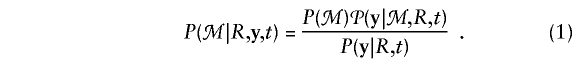
We define a family to be a set of individuals such that (a) any two individuals are connected in the sense proposed by Thompson (1986, p 21) and (b) each individual is either a founder (neither parent belongs to the family) or a nonfounder (both parents belong to the family). The genotype and/or phenotype of any family member may be unknown; however, the family must contain at least one member with a known phenotype and at least one member with a known genotype. Let y=(y₁,...,y_m) denote the vector of phenotypes for the m members with known phenotype. Here y_ℓ has a value of 1 if the ℓth family member is affected with the disease and has a value of 0 otherwise, ℓ=1,...,m. We assume that phenotypes are missing at random (Little and Rubin 1987)—that is, the probability of failure to observe a member’s disease status does not depend on his or her actual status or on his or her marker genotypes. With this assumption, the likelihood at locus t is the probability P(ℳ|R,y,t) of the family’s observed marker data, denoted as ℳ, given the family’s geneological structure R, given the vector y of observed phenotypes, and given that t is the disease locus. We use Bayes theorem to write this probability as follows:

To simplify the notation, we now suppress the dependence of the probabilities both on the family structure R and on the particular locus t. Let g=(g₁,...,g_m) denote the vector of genotypes at locus t of the m family members of known phenotype. We want to allow for the possibility that t is not one of the marker loci. Assumption A.1 states that the family’s phenotype y and its marker data ℳ are conditionally independent, given g. Thus, we write

where denotes summation over all possible genotype vectors g. Substitution of notation (2) into probability (1) gives the likelihood for the family as

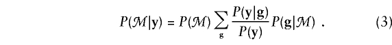In this instance, P(y)=Σ_gP(y|g)P(g) is the marginal probability of the family phenotype.

Family likelihood (3) involves three types of probabilities. The first type is the probability P(ℳ) of the family’s marker data, under the null hypothesis that the chromosomal region containing the markers is not related to disease risk. We shall specify this probability in terms of a vector of marker parameters. These determine the frequencies of the marker alleles or haplotypes among chromosomes in the populations from which the family’s founders were drawn, and we assume that they are known.

The second type of probability relates the alleles at locus t to the marker data. These probabilities appear in expression (3) as P(g|ℳ). They depend on the extent of gametic disequilibrium between locus t and the marker loci in the family founders and on the probability of recombination between t and its nearest marker loci in meioses within a family. In general, the extent of gametic disequilibrium between markers and t is not known, unless t is one of the marker loci. However, in many situations of practical interest, the test statistics themselves do not depend on this gametic disequilibrium, although their power does.

The third type of probability needed in the likelihood consists of the penetrance functions P(y|g) for the various possible family genotypes g. For family members with known phenotype, these penetrance functions give the joint probability of disease occurrence or nonoccurrence as functions of the members' genotypes at locus t. To specify these penetrances, we assume that, at most, one allele or one group of alleles, labeled D₁, confers elevated disease risk. We also group all other alleles and label this group as allele D₂. We set g=i for the genotype of an individual who carries i copies of the putative high-risk allele D₁, i=0,1,2.

For families with one individual of known phenotype, we need only the three penetrances P(y=1|g=i), i=0,1,2. We shall consider the following general class of penetrance models:

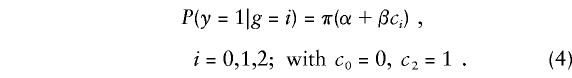Here π is a known smooth monotonic function, α is a constant that specifies risk in D₂D₂ homozygotes, and β is an unknown constant relating risk in D₁D₁ homozygotes to that in D₂D₂ homozygotes. Also, c₁ is a specified constant relating disease risk in D₁D₂ heterozygotes to that in D₂D₂ homozygotes. The value β=0 corresponds to the null hypothesis of no relation between the disease and locus t. In this instance, the parameter α determines the disease prevalence in the population π(α), under the null hypothesis that disease is unrelated to the family genotype g. We will often assume that π(α) is known from data on disease prevalence in the population. We shall call α and β “penetrance parameters.”

Penetrance has traditionally been modeled with the use of π(x)=x, with c₁=1 for the dominant model, c₁=0 for the recessive model, and c₁=1/2 for the additive model. Other models in the class (4) include the multiplicative model, with π(x)=exp(x) and c₁=1/2 (Self et al. 1991; Risch and Merikangas 1996; Schaid 1996; Whittaker and Lewis 1998), and the linear logistic model, with π(x)=e^x/(1+e^x) and c₁=1/2 . The penetrances in any model (4) with c₁=1/2 are, after an appropriate transformation, linear in the number i of high-risk D₁ alleles. Accordingly, we shall call them “GLMs” (McCullagh and Nelder 1989). Individuals with genotype g at a putative trait locus t will be said to have a “D₁ count of c_g.” Thus, if the penetrances are specified by a GLM, an individual’s D₁ count is one-half of the number of his or her copies of allele D₁. In contrast, for a recessive or dominant model, an individual’s D₁ count is 1 if he or she is a carrier of the high-risk genotype; otherwise, it is 0.

For families with m>1 members of known phenotype, we must specify their joint probability of disease, conditional on their genotypes at locus t. We assume that, given his or her own genotype g, an individual's phenotype does not depend on the genotypes of his or her relatives and that, given g, the phenotypes of relatives are conditionally independent. Therefore,

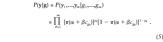These assumptions ignore the possibility that residual correlation in family phenotypes may be a result of other loci responsible for the disease or of shared, unmeasured risk factors. Fortuitously, the proposed statistical tests remain valid (in the sense of having the correct null asymptotic p values) even if this residual correlation is ignored, and we shall ignore it hereafter. However, it is possible that more-accurate modeling of the correlation could improve statistical power, and this possibility requires investigation.

From (5), we see that, under the null hypothesis β=0, the probability P(y|g) is independent of the family genotype g; thus, the likelihood (3) is simply the null probability P(ℳ) of the marker data. Our objective is to derive efficient score statistics based on the likelihood (3) and to use them to test the null hypothesis β=0 for various test loci t in the region covered by the markers. When assumption A.1 holds, the score statistics have standard Gaussian null distributions—asymptotically, as N→∞. After presentation of the statistics, we will discuss, in brief, the types of bias that can arise when assumption A.1 fails.

Score for a Family

We consider the use of likelihood-based efficient score statistics (Cox and Hinkley 1974) for testing of the null hypothesis that a family’s phenotype y is independent of its genotype g at locus t—that is, β=0. To describe these statistics, we suppose that there are K possible categories of marker genotypes for the family and that, if the marker genotypes were known for all members, the family could be classified in one and only one of the categories. For example, table 1 shows the K=15 categories for a nuclear family with one offspring, when the marker data consist of genotypes at a single diallelic locus. In general, the family’s marker category may not be known, because some members have not been typed at some or all of the marker loci. To deal with this uncertainty, we shall introduce a random variable x_k that represents the null probability that the family has category k, given its observed marker data ℳ:

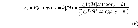In this instance, r_k is the marginal probability that the family belongs to category k, under the null hypothesis. If the family is known to have, for example, category ℓ, then x_ℓ=1 and x_k=0, k≠ℓ. If the category is not known, then x_k is a conditional probability, given the marker data.

Table 1.

K=15 Categories of a Diallelic Autosomal Marker for a Nuclear Family with One Offspring

	Probabilityb
Marker Category (k=fh=f1f2h)a	uf	vh|f	C1kC2kC3kc	wkd
1. B1B1,B1B1,B1B1 (222)	u22	1	111	2-ψ
2. B1B1,B1B2,B1B1 (212)	u1u2	1/2	1c11	2-ψc1
3. B1B1,B1B2,B1B2 (211)	u1u2	1/2	1c1c1	1-ψc1+c1
4. B1B2,B1B1,B1B1 (122)	u1u2	1/2	c111	c1-ψ+1
5. B1B2,B1B1,B1B2 (121)	u1u2	1/2	c11c1	2c1-ψ
6. B1B1,B2B2,B1B2 (201)	u0u2	1	10c1	1+c1
7. B2B2,B1B1,B1B2 (021)	u0u2	1	01c1	-ψ+c1
8. B1B2,B1B2,B1B1 (112)	u21	1/4	c1c11	(1-ψ)c1+1
9. B1B2,B1B2,B1B2 (111)	u21	1/2	c1c1c1	(2-ψ)c1
10. B1B2,B1B2,B2B2 (110)	u21	1/4	c1c10	(1-ψ)c1
11. B1B2,B2B2,B1B2 (101)	u1u0	1/2	c10c1	2c1
12. B1B2,B2B2,B2B2 (100)	u1u0	1/2	c100	c1
13. B2B2,B1B2,B1B2 (011)	u0u1	1/2	0c1c1	(1-ψ)c1
14. B2B2,B1B2,B2B2 (010)	u0u1	1/2	0c10	−ψc1
15. B2B2,B2B2,B2B2 (000)	u20	1	000	0

^af_i = number of B₁ alleles in the genotype of parent i, i=1,2; h = number of B₁ alleles in genotype of the offspring.

^bu_f=u_f1f2 = probability of parental genotype f=f₁f₂; v_h|f = probability of offspring genotype h, given parental genotype f.

^cC_ℓk = D₁ count of family member ℓ, ℓ=1,2,3, when family has category k and when D₁=B₁.

^dw_k=a₁C_1k+a₂C_2k+a₃C_3k, where a_ℓ is a phenotype value for family member ℓ, ℓ=1,2,3.

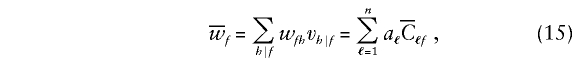
In the Appendix, we show that, for the class (4) of penetrance models and on the basis of the likelihood (3) at locus t, the score for the family is

Here w_k is a weight attached to marker category k. Thus, the score is a weighted sum of deviations between “observed” and expected frequencies of the K marker categories. The weights w_k determine the importance of one marker category relative to another. They depend on the relations between genotypes at marker loci and genotypes at locus t as well as on the penetrance functions relating disease to genotypes at t.

To describe the weights, we consider the simple example of a nuclear family with one offspring evaluated at a single diallelic “candidate gene” with alleles B₁=D₁ and B₂=D₂ and with no missing genotypes or phenotypes. In table 1, the Marker Category column shows the 15 possible marker categories for the family, where f₁, f₂, and h denote the genotypes of parent 1, parent 2, and the offspring, respectively. For category k=f₁f₂h, the penetrance values c₂, c₁, and c₀ determine a triple value, C_1kC_2kC_3k=c_f1c_f2c_h, of D₁ counts for the family. The C_1kC_2kC_3k column in table 1 shows these triple values for c₂=1 and c₀=0. The weight w_k for category k is

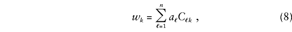where C_ℓk is the D₁ count of family member ℓ when the family has marker category k, ℓ=1,...,n, and n=3 in this example. Also, a_ℓ, a phenotype value for member ℓ, is defined as follows:

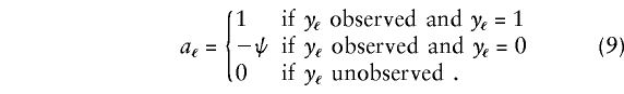In this definition, ψ=π/(1-π), where π=π(α) is the disease prevalence in the population under the null hypothesis. If, for example, parent 1 and the offspring are affected and parent 2 is unaffected, then a₁=a₃=1 and a₂=-ψ. Substitution of these values in (8) results in w_k=C_1k+C_3k-ψC_2k. Thus, w_k is a difference between D₁ counts of affected and unaffected family members, with unaffected family members contributing a value ψ, relative to affected members. In table 1, the w_k column shows the weights w_k for the 15 marker categories.

The marker category probability r_k in score (7) factors as the probability of the founder-genotype category multiplied by the conditional probability of the nonfounder-genotype category, given the founder-genotype category. Thus, a specific marker category can be written as k=fh, where f and h represent categories of marker genotypes for founders and nonfounders, respectively. For example, the family genotype B₁B₁,B₁B₂,B₁B₁ (table 1, row 3 [B₁B₁,B₁B₂,B₁B₂ {211}] ) is labeled f=21 and h=1 or k=fh=211. We write

where u_f is the null probability of founder category f and where v_h|f is the probability of nonfounder subcategory h, given that the founders’ genotypes belong to category f. The Probability column of table 1 shows u_f and v_h|f for the nuclear family in this example. Notice that the probabilities r_k depend on the marker parameters only through u_f; the probabilities v_h|f are constants determined by the Mendelian laws of inheritance.

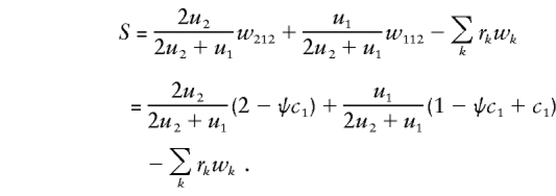
To illustrate computation of the score S, suppose that the nuclear family is observed to have marker category f₁f₂h=212. Then, from equation (6), x₂₁₂=1 and x_k=0, k≠212. Substitution of these values into equation (7) gives the score for this family as S=w₂₁₂-Σ_kr_kw_k. From equation (8), we see that the score is the difference between the observed and expected values of a linear combination of D₁ counts among the family members.

In row 2 (B₁B₁,B₁B₂,B₁B₁ [212]) of table 1, w₂₁₂=2-ψc₁. Also, from equation (8) and from the values for r_k in table 1, Σ_kr_kw_k=Σ³_ℓ=1a_ℓ(Σ_kr_kC_ℓk)=(a₁+a₂)(u₂+c₁u₁)+a₃(u^′₂+c₁u^′₁), where u^′₂=(u₂+ 1/2u₁)² and u^′₁=u₁+2u₀u₂- 1/2u²₁. Thus, . Under Hardy-Weinberg equilibrium (HWE) for the parental-genotype frequencies, u₂=u^′₂=[P(B₁)]² and u₁=u^′₁=2P(B₁)P(B₂). If, in addition, c₁=1/2, then S=2- 1/2ψ-(2-ψ)P(B₁).

Suppose that parent 1 is untyped. We therefore know only that the family marker category is either 212 or 112. Thus, according to equation (6) and rows 2 and 8 (B₁B₁,B₁B₂,B₁B₁ [212] and B₁B₂,B₁B₂,B₁B₁ [112], respectively) of table 1,

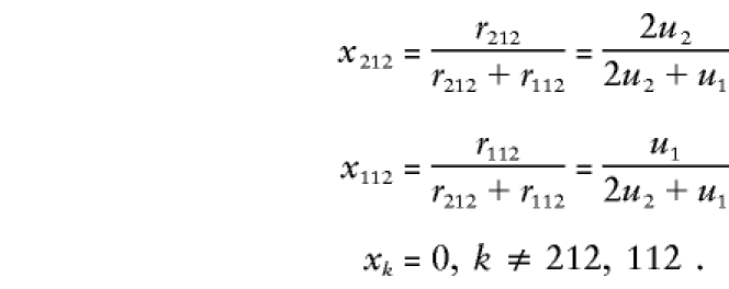Under HWE, x₂₁₂=P(B₁) and x₁₁₂=P(B₂). The family’s score is as follows:

In general, when some family members are untyped, a random vector of probabilities (6) is assigned to the possible categories, where the probabilities are conditional on the observed marker data for the family. This random vector depends on the null founder-genotype probabilities u_f, which must be specified or estimated from external data. In the companion article (Tu et al. 2000), we illustrate maximum-likelihood estimation of u_f when the founders are parents in nuclear families. Martin et al. (1998) have also proposed such genotype reconstruction for parents in nuclear families.

We will now describe the weights w_k for families of arbitrary structure, not only when some members may be untyped but, also, when the markers do not necessarily include the trait locus. To do so, we will let γ_ℓk(i) denote the probability that member ℓ of a family with marker category k carries i copies of allele D₁, i=0,1,2. The weights are then given according to equation (8), where C_ℓk=c₁γ_ℓk(1)+γ_ℓk(2) is now the conditional D₁ count for family member ℓ, given the family marker category k. When, as in the example shown in table 1, the marker data include genotypes at locus t, a family marker category k specifies a D₁ count for each family member.

In summary, computation of a family’s score S may involve two types of imputation: (a) imputation of the family marker category when it is incompletely observed (e.g., when parental genotypes are missing) and (b) imputation of family members’ D₁ counts at the putative disease locus t, when locus t is not one of the markers. The latter imputation requires knowledge of the extent of disequilibrium between locus t and its nearest markers among the family founders. Like the disease prevalence π, disequilibrium parameters relating alleles at locus t to those at the marker loci cannot be estimated from the data, since genotypes at locus t are not observed. However, misspecification of the disequilibrium parameters will not affect the validity of a score test, although it will decrease the test’s power.

Expressions (8) and (9) indicate that the contribution of an unaffected member, relative to that of an affected member, is determined by the disease odds ψ=π/(1-π). Since the disease prevalence π is invariably <1/2, the counts of unaffected members contribute less to the score than do those of affected members. In particular, for rare diseases (π≪1), the counts of unaffected members contribute little to the score statistic. For many diseases, π is known at least approximately. It cannot be estimated from the family data, since the families have been ascertained on the basis of their phenotype. However, since π appears only in the weights w_k and not in the null probabilities r_k, its misspecification will not produce incorrect p values, although it may affect statistical power. Choosing optimal values for ψ is an area that requires research. In the companion article (Tu et al. 2000), we use simulations to compare the power of tests based on genotypes in phenotype-discordant sib pairs, with the use of ψ=1 and ψ equal to the disease odds in the population.

Under the null hypothesis, the score S of equation (7) has a mean of 0 and an asymptotic variance of

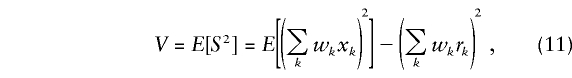as described in the Appendix.

Decomposition of the Score

The factorization (10) of the null family marker category probabilities r_k of induces a decomposition of the score (7) as a sum of nonfounder and founder scores: S=S_NF+S_F. In this instance, the nonfounder score is

where denotes summation over the nonfounder categories h compatible with f, w_fh=w_k, and x_fh=x_k when fh=k, and with .

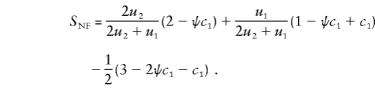
For the family with observed marker category 212 (see table 1), we have x_21•=1 and x_f•=0 when f≠ 21. Substitution of these values and the corresponding v_h|f into equation (12) results in the following nonfounder score for this family: S_NF=w₂₁₂- 1/2(w₂₁₂+w₂₁₁)= 1/2(w₂₁₂-w₂₁₁). For the phenotype values (a₁,a₂,a₃)=(1,-ψ,1), w₂₁₂ and w₂₁₁ are shown in rows 2 and 3 (B₁B₁,B₁B₂,B₁B₁ [212] and B₁B₁,B₁B₂,B₁B₂ [211], respectively) of table 1. With these values, S_NF=2-ψc₁- 1/2(3-2ψc₁+c₁)= 1/2(1-c₁). Marker category 212 denotes transmission of allele B₁ from heterozygous parent 2 to the affected offspring. If this parent had transmitted allele B₂ to the affected offspring, resulting in marker category 211, then the NFS would be S_NF= 1/2(c₁-1). Thus, if c₁=1/2, then S_NF=1/4 or -1/4, depending on whether parent 2 transmits allele B₁ or B₂ to the offspring. Indeed, for a single marker in nuclear families with known genotypes and c₁=1/2, S_NF is just the TDT.

Notice that the parental-phenotype values do not contribute to S_NF. In general, founders contribute only their genotypes to the NFS, and these founder genotypes are used only to compute the null expectations of the nonfounder genotypes. In contrast, phenotypes of nonfounders play a central role in the statistic. If, for example, the phenotype of the single offspring in this family were unknown, then S_NF would vanish. The genotypes of nonfounders with unknown phenotype are useful for reconstruction of the family’s marker category, but, because they do not enter the weights w_k, they are not evaluated directly in the NFS.

When the genotype of parent 1 is unknown, the nonfounder score is as follows:

As this example illustrates, when the founder category of the family is known, S_NF does not involve the marker parameters. However, when the founder category is not known, S_NF depends on the marker parameters through the founder-category probabilities u_f, which, in formula (6), determine the r_k for the x_k.

The variance of S_NF, conditional on the vector x_•=(x_1•,...,x_F•) of probabilities for the F founder categories, is as follows:

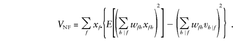We now turn to the founder score, which is as follows:

In this case,

and is the expected D₁ count for the ℓth member in a family whose founders have marker category f. Consider again the family with category 212 (see table 1), so that x_21•=1 and x_f•=0 when f≠21. For this family, . From equation (15), we see that, with phenotype values (a₁,a₂,a₃)=(1,-ψ,1),

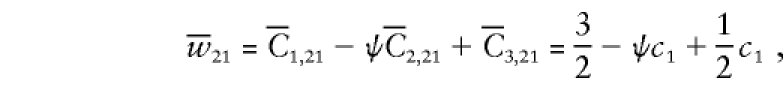where we have used the expected D₁ counts , and . Two observations are noteworthy in this case: (a) the expected D₁ counts for the founder parents are just their observed D₁ counts, whereas the D₁ count of the offspring is his or her expected count, given those of his or her parents, and (b) if, for example, parent 1 has a known genotype but an unknown phenotype—so that a₁=0—then the genotype of this parent still contributes to the founder score through its contribution to the expected D₁ count of his or her affected offspring. In contrast, if the offspring has a known genotype but an unknown phenotype, his or her genotype is used only to reconstruct the genotypes of his or her parents.

The variance of S_F is as follows:

The variance of the total score, given by equation (11), can be written as follows:

where E[V_NF] is given by equation (13), with x_f• replaced with u_f.

Score Statistic for N Families

For a collection of N independent families from a population that is homogeneous with respect to disease risk, the nonfounder, founder, and total score statistics are, respectively,

In this case, for the νth family, ν=1,...,N, V_NFν, V_Fν, and V_ν, are given by (13), (16), and (17), and the hat denotes an estimate. (In these expressions, the unknown parameters u_f must be replaced with estimates.) When the founder-genotype probabilities are specified correctly, the statistics 𝒯, 𝒯_NF, and 𝒯_F in (18) each have—asymptotically, as N→∞—a standard Gaussian distribution under the null hypothesis of no effect at locus t.

The score statistics for N families from a population that is heterogeneous with respect to disease risk are the weighted averages of statistics for the I homogeneous subpopulations. For example, the total score statistic is , where, for subpopulation i, 𝒯_i is the total score statistic and where the weight ε_i depends on its disease risk in the population π_i, as described in the Appendix.

Some invariance properties of the score statistics are worth noting. First, a family’s founder score S_Fν in (14) is unchanged if all weights are replaced with , where ξ_ν is an arbitrary family-specific constant, since . Second, the nonfounder score S_NFν in (12) is unchanged when all weights w_νfh are replaced by w^*_νfh=w_νfh+ξ_νf, where ξ_νf is an arbitrary family-specific constant that is independent of its nonfounder category h. In particular, since the conditional D₁ counts of founders depend only on their own category f and not on the category h of their descendants, the summands of w_νfh corresponding to founders can be ignored. Therefore, neither the D₁ counts nor the phenotypes of founders contribute to the NFS. Finally, the weights in either the founder score or the nonfounder score can all be multiplied by any nonzero constant ξ, without changing the standardized test statistics. We shall use these invariance properties to simplify the test statistics in the examples in this article and in the companion article (Tu et al. 2000).

We conclude this section with a brief discussion of the bias (i.e., incorrect asymptotic type I–error probabilities) that could arise if assumption A.1 fails. This assumption states that, given the family’s genotypes at a test locus t, its phenotypes and marker genotypes are independent. It would fail if one or more of the markers were associated with any (genetic or nongenetic) risk factors for the disease. In this case, the likelihood at locus t, under the null hypothesis β=0, would not be the null probability of the markers in the general population, since the families were ascertained for multiple cases of disease. Consequently, the FS, which compares the genotype frequencies among founders in these multiple-case families with those in some reference population, would not have a standard Gaussian distribution. Thus, the FS can be biased by association between markers and risk factors that do not segregate with disease within families. The NFS, in contrast, is conditioned on the observed or inferred distribution of marker genotypes in the founders of the ascertained families. This conditioning assures that the NFS has the correct asymptotic null distribution in the absence of linkage to a locus that segregates with disease within families, provided that, when some founder genotypes are unobserved, the distribution of founder genotypes is specified correctly. While departures from random mating, HWE, etc., in the founders could, in principle, affect the asymptotic null distribution of the NFS, it is difficult to envisage examples involving serious bias. Most likely, divergent results for NFS and FS at a given locus t, with the former being nonsignificant and the latter significant, would suggest marker-disease association in the absence of linkage. Conversely, if the NFS were significant but the FS were nonsignificant, then this would suggest that the markers are linked to, but are in weak gametic disequilibrium with, a disease locus t.

Application to Single Diallelic Polymorphisms in Case Series and Case-Control Studies

We illustrate the score statistics by applying them to very simple families, such as nuclear families and “families” consisting of single unrelated individuals. We regard a single individual, who is either affected (a case) or unaffected (a control), as a founder of his or her “family.” The scores of nuclear families and of unrelated cases and controls are summed to form the test statistics. The FS T_F evaluates the genotypes of cases, controls, and parents in the nuclear families, whereas the NSF T_NF evaluates just the genotypes of the offspring in the nuclear families, comparing them with the Mendelian expectation.

Suppose that individuals are typed at a single diallelic marker with alleles B₁ and B₂. The marker locus may be distinct from the test locus t, but, if this is so, then the alleles at the two loci are assumed to be in gametic disequilibrium in the population. Let P(D_iB_j) denote the probability that a random chromosome from the population carries the haplotype D_iB_j, i, j=1, 2. Table 2 gives these probabilities in terms of the marginal probabilities P(D_i) and P(B_j) and the disequilibrium coefficient δ=P(D₁B₁)-P(D₁)P(B₁). The probability p₁ that a random chromosome containing allele B₁ also contains allele D₁ is thus

The analogous probability p₂, for a chromosome containing B₂, is

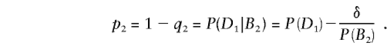For convenience, we introduce a standardized disequilibrium coefficient Δ, defined as . By assumption, Δ≠0.

Table 2.

Haplotype Probabilities at Test Locus t and Marker Locus s

	Haplotype Probability at Marker Allele
Disease Allele	B1	B2	Total
D1	P(B1)P(D1)+δ	P(B2)P(D1)-δ	P(D1)
D2	P(B1)P(D2)-δ	P(B2)P(D2)+δ	P(D2)
Total	P(B1)	P(B2)	1

In the companion article (Tu et al. 2000), we applied the score statistics to nuclear families for which markers at the putative disease locus are observed but for which the family marker category typically is unobserved. In contrast, in the present study, we apply them to families consisting of single, unrelated individuals in which the marker category is observed but in which the marker may not be the trait locus. Since these latter families contain only founders, the nonfounder score is 0, and the total score for an individual reduces to the founder score S_F of (14). There are K=F=3 marker categories—namely, the three genotypes B₂B₂, B₁B₂, and B₁B₁—which are indexed as f=0,1,2, respectively. Their null probabilities are r_f=u_f, f=0,1,2.

Case Series

In case series, the marker genotypes of a sample of N cases are compared with those in some reference population. The score statistic is given by (14), with the weight for a case with genotype f given as , as shown in table 3. The invariance properties of the test statistic, which were described at the end of the previous section, allow us to standardize the weights so that w₀=0 and w₂=1. Note, however, that this standardization requires replacement of with , where . Since is proportional to the disequilibrium coefficient Δ, the standardization is possible only when Δ≠0. Indeed, S_F is itself proportional to Δ. Thus, if Δ=0—that is, if the marker were in linkage equilibrium with the test locus, then the distribution of the FS would be degenerate at 0.

Table 3.

Probability That a Founder with f Copies of Marker Allele B₁ Carries i Copies of a Nearby Disease Allele

f					a
2	q21	2p1q1	p21	2c1p1+ep21b	1
1	q1q2	p1q2+q1p2	p1p2	c1(p1+p2)+ep1p2	λc
0	q22	2p2q2	p22	2c1p2+ep22	0

^a, if and only if Δ≠0, where Δ=p₁-p₂ is the standardized disequilibrium coefficient.

^be=1-2c₁.

^c.

In table 3, we see that the weight attached to B₁B₂ heterozygotes, when B₁B₁ and B₂B₂ homozygotes receive weights of 1 and 0, respectively, is λ, which is defined as follows:

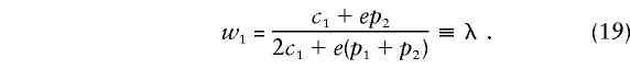Here e=1-2c₁. We use the symbol S_Fν to denote the founder score for the νth case. Substitution of the weights (19) into equation (14) results in

where u_f is the frequency of genotype f in the reference population and where x_νf=1; otherwise, if the case’s genotype is f, x_νf=0, f=0,1,2. Summing the individual scores (20) over the N cases shows that the score is Σ^N_ν=1S_Fν=N₂+λN₁-N(u₂+λu₁), where N_f is the number of cases with genotype f. The founder (and total) score statistic is

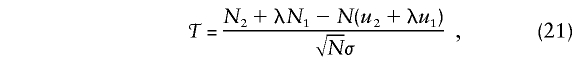where, from (16),

To use 𝒯, we must specify the weight λ for heterozygotes and the genotype frequencies u₀,u₁,u₂ in the reference population.

Case-Control Studies

Case-control studies are based on comparison of the marker genotypes of, for example, N_𝒜 cases with those of N_𝒰 controls. The likelihood for the data is the product of the probabilities of case and control marker data, and the corresponding score is the sum of the score for the case data plus the score for the control data. The resulting test statistic can be written as

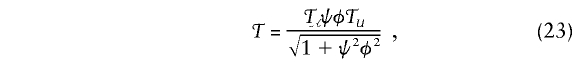where 𝒯_𝒜 and 𝒯_𝒰 are the test statistics (21) applied to cases and controls, respectively; where ψ is the phenotype value for controls in equation (9); and where φ²=N_𝒰/N_𝒜 is the control:case ratio.

To use 𝒯, we must specify the heterozygote weight λ of equation (19), the phenotype value ψ, and the null marker genotype probabilities u₀,u₁,u₂. With the choice of ψ=N_𝒜/N_𝒰, equation (23) becomes

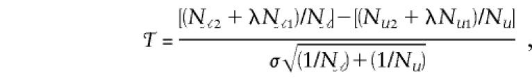where N_𝒜g and N_𝒰g are the numbers of cases and controls, respectively, with genotype g=0,1,2 and where σ² is given by (22). This choice for ψ eliminates the null genotype frequencies u₀,u₁,u₂ from the numerator of 𝒯; however, they appear in σ. They can be estimated from the group of controls as . The resulting test statistic 𝒯 is the standardized difference in expected D₁ counts between cases and controls. For c₁=1/2, 𝒯 is the statistic proposed by Barcellos et al. (1997) and Risch and Teng (1998), for testing of allelic association between disease and marker in pooled DNA from cases and controls. In this case, 𝒯 also is the score statistic for the traditional linear logistic regression of unrelated cases and controls.

Heterozygote Weight λ

The optimal weight λ for heterozygotes varies according to the penetrance model and the extent of disequilibrium between trait and marker loci, as specified by the probabilities p₁ and p₂. In practice, these probabilities seldom are known. However, it is evident from (19) that, for c₁=1/2, the weight is λ=1/2, independent of p₁ and p₂. For these models, 𝒯 is just the standardized difference between observed and expected B₁ counts, regardless of the extent of gametic disequilibrium between the two loci (provided, of course, that some disequilibrium exists).

When trait and marker loci coincide (so that, for example, p₂=0, p₁=1), then λ=c₁. In this case, 𝒯 is the standardized difference between observed and expected B₁ counts in cases and controls. If trait and marker loci do not coincide and if c₁≠ 1/2, then the extent of disequilibrium between trait and marker loci can have a large influence on the heterozygote weight λ. For a dominant model (c₁=1), equation (19) shows that λ=q₂/(q₁+q₂), which is closer to 1/2 than to 1 when the disease allele is rare. For a recessive model (c₁=0), equation (19) shows λ=p₂/(p₁+p₂), which varies from 0 (when the disease allele and allele B₁ are in complete disequilibrium) to 1 (when the disease allele and allele B₂ are in complete disequilibrium).

Suppose, for example, that the frequency of the disease allele is .01 and that the two marker alleles are equally likely. Then, for maximum disequilibrium between disease and marker loci, λ=0 for a recessive disease gene and λ=.505 for a dominant gene. If the disequilibrium coefficient δ equals one-fourth of its maximum value, then λ=.25 for a recessive gene and .503 for a dominant gene. Thus, when disease and marker loci do not coincide, the optimal weight λ for heterozygotes is not 0 for a recessive gene and 1 for a dominant gene. For rare disease alleles, it is always ∼1/2, when the disease allele is dominant. For common disease alleles, the optimal weight can strongly depend on the tightness of disequilibrium, regardless of the mode of inheritance. For instance, when the disease-allele frequency is .2, then, under maximum disequilibrium, λ=0 for a recessive model and λ=.63 for a dominant model. However, for loose disequilibrium (δ equal to one-fourth of its maximum value), λ=.38 for a recessive model and λ=.53 for a dominant model. Lack of knowledge concerning both the extent of gametic disequilibrium and the correct penetrance model suggests use of the value λ=1/2 in the test statistic (21). There is a need for investigation of the power associated with use of this strategy, for a range of situations.

Discussion

We have described a likelihood-based score statistic for detection of disease genes by evaluation of phenotype-marker associations and transmission disequilibrium within families. The score statistic decomposes into two components, the NFS and the FS. These components represent two types of deviation between observed genotypes and their expectations under the null hypothesis. Each will have a large absolute value if the chromosomal region contains a disease locus and if the families have been selected to contain affected individuals. The NFS represents the deviation between observed and expected marker alleles in nonfounders, given the founder genotypes. It reflects transmission disequilibrium from parent to affected and unaffected offspring, and it will be large because the disease locus is linked to the markers. When the marker data consist of genotypes at a single locus, both the nonfounder and founder scores are proportional to the standardized disequilibrium coefficient Δ between marker and disease loci. Thus, the statistics should be used only to evaluate the etiologic relevance of loci t that are in linkage disequilibrium with the marker. In addition, the nonfounder score is proportional to 1-2θ, where θ is the probability of recombination between the marker and disease loci. Thus, if the two loci were unlinked (θ=1/2), then the nonfounder score would vanish identically, and the marker genotypes of nonfounders would not contribute to the total test statistic. If, on the other hand, θ=0, which would hold when we wish to test the etiologic relevance of the marker itself, then founders and nonfounders contribute equally to the total test statistic. In this sense, the genetic distance between marker and disease loci, as measured by their recombination fraction θ, determines the relative contributions of founder and nonfounder genotypes to the total test statistic.

The FS evaluates association between disease and marker alleles in family founders, and it extends the test statistics that are currently used for the analysis of case-control data. FS reflects deviation between the observed or inferred frequencies of marker genotypes in the founders and those that are expected in the general populations to which they belong. It measures association between the disease and the disease locus, and it will be large when there is gametic disequilibrium between disease and marker loci among the founder chromosomes. If the null founder-genotype frequencies can be estimated from independent data, then the FS provides information supporting or refuting the null hypothesis derived from the (observed or inferred) marker genotypes of the founders, even when their phenotypes are unknown. However, the FS also can be large because of population stratification or inappropriate assumptions (e.g., random mating or Hardy-Weinberg proportions) on the distribution of founder genotypes. Thus, the FS tests for association, whereas the NFS tests for linkage as the cause of the association.

These likelihood-based statistics have certain strengths and limitations. Because they are model-based, they clarify the role of the underlying genetic model in the determination of the weights for affected versus unaffected individuals and, when dealing with single diallelic markers, the weights for heterozygotes versus homozygotes. When the model is correctly specified, the statistics enjoy certain local asymptotic optimality properties (Cox and Hinkley 1974). However, the model requires assumptions about the distribution of the founder genotypes, and the effects on bias and power resulting from departures from these assumptions have not yet been fully evaluated. There is a need to assess the impact on bias and power loss associated with misspecification of the distribution of founder genotypes. One might expect that this impact would be small when the founder genotypes are known or can be inferred with some confidence.

One strength of the statistics is that they apply to any type of family structure, including a “family” consisting of a single individual, and that they thus eliminate the need for many different ad hoc tests. In addition, the approach provides a strategy for dealing with missing phenotypes and genotypes for key family members, such as parents. Also, when it is applied to families in which the phenotypes of some founders are known, the FS allows comparison of genotypes of affected and unaffected founders. Simultaneous evaluation of the FS (which may be biased by population stratification) and the NFS (which is less vulnerable to such bias) can provide insight into the etiologic relevance of observed associations.

The likelihood-based framework presented in this study stimulates consideration of several potentially useful extensions. First, the likelihood could be extended to accommodate censored survival data rather than binary disease outcomes. Second, the likelihood could be modified to include nongenetic covariates, in the manner considered by Self et al. (1991). In fact, the likelihood function proposed by Self et al. is a special case of the nonfounder component of the likelihood considered in the present study. Inclusion of nongenetic covariates would lead to score statistics that have been adjusted for the effects of the covariates. In addition, joint maximization of the likelihood, with respect to regression coefficients for both genetic markers and nongenetic factors, would allow for multivariate estimation of genotype relative risks (Schaid and Sommer 1993; Schaid and Li 1997; Witte et al. 1999).

If it becomes feasible to produce reliable estimations of both intermarker genetic distances and population-specific intermarker disequilibrium coefficients, then association studies will benefit from simultaneous consideration of multiple markers that may flank a disease locus. The systematic framework presented here should prove useful for such studies.

Appendix

We derive the score statistic for a family with phenotype y=(y₁,...,y_m), where m is the number of members with known phenotype. Suppose that there are K categories of marker genotypes. Let r_k denote the family’s null probability of having category k, and let x_k=P(k|ℳ) denote its conditional probability of having category k, given its observed marker data ℳ. The likelihood (3) for the family can therefore be written as follows:

P(g|k) is the probability that a family with marker category k has genotype g at the disease locus t. Also, Θ is a vector of parameters that includes the penetrance parameters α and β, any unknown marker parameters in the probabilities r_k, and the test-locus-vs.-marker parameters. Let be a null value of Θ—that is, one for which β=0 and for which the remaining parameters are specified under the null hypothesis. By differentiation of the logarithm of (A1), with respect to β, and by evaluation of the same logarithm at , we find, after some algebraic calculations, that the family’s score is as follows:

In this instance, is the logarithmic derivative of the null disease prevalence in the population, and w_k is a nonnegative constant, as described in equations (8) and (9).

The null mean of S is 0, which follows from likelihood theory (Cox and Hinkley 1974). This can also be seen from equation (7) and from the fact that the null mean of the random variable

is

denotes summation over all possible realizations of the observed marker data ℳ.

The asymptotic variance of the score εS (Cox and Hinkley 1974) is

For N families from a population that is homogeneous with respect to disease risk π, the score statistic is . If the families are sampled from a heterogeneous population consisting of I identified subpopulations with disease risks π_i, i=1,...,I, then , where and where 𝒯_i is the score statistic for the subset of families from population i. In the present study, we assume that the population is homogeneous, so that ε_i≡ε, i=1,...,I, and we may take ε=1 without loss of generality.

Note added in proof.—Further discussion of likelihood-based methods analogous to the methods presented here can be found in a study by Clayton (1999).

References

- Barcellos LF, Klitz W, Field LL, Tobias R, Bowcock AM, Wilson R, Nelson MP (1997) Association mapping of disease loci, by use of a pooled DNA genomic screen. Am J Hum Genet 61:734–747 [DOI] [PMC free article] [PubMed] [Google Scholar]
- Clayton D (1999) A generalization of the transmission/disequilibrium test for uncertain-haplotype transmission. Am J Hum Genet 65:1170–1177 [DOI] [PMC free article] [PubMed] [Google Scholar]
- Cox RDR, Hinkley DV (1974) Theoretical statistics. Chapman and Hall, London [Google Scholar]
- Ewens WJ, Spielman RS (1995) The transmission/disequilibrium test: history, subdivision, and admixture. Am J Hum Genet 57:455–464 [PMC free article] [PubMed] [Google Scholar]
- Knapp M, Seuchter SA, Bauer MP (1993) The haplotype-relative-risk (HRR) method for analysis of association in nuclear families. Am J Hum Genet 52:1085–1093 [PMC free article] [PubMed] [Google Scholar]
- Little RJA, Rubin DB (1987) Statistical analysis with missing data. John Wiley & Sons, New York [Google Scholar]
- Martin RB, Alda M, MacLean CJ (1998) Parental genotype reconstruction: applications of haplotype relative risk to incomplete parental data. Genet Epidemiol 15:471–490 [DOI] [PubMed] [Google Scholar]
- McCullagh P, Nelder JA (1989) Generalized linear models, 2d ed. Chapman and Hall, London [Google Scholar]
- Ott J (1989) Statistical properties of the haplotype relative risk. Genet Epidemiol 6:127–130 [DOI] [PubMed] [Google Scholar]
- Parsian A, Todd RD, Devor EJ, O’Malley KL, Suarez BK, Reich T, Cloninger CR (1991) Alcoholism and alleles of the human D2 dopamine receptor locus: studies of association and linkage. Arch Gen Psychiatry 48:655–663 [DOI] [PubMed] [Google Scholar]
- Risch N, Merikangas K (1996) The future of genetic studies of complex human diseases. Science 273:1516–1517 [DOI] [PubMed] [Google Scholar]
- Risch N, Teng J (1998) The relative power of family-based and case-control designs for linkage disequilibrium studies of complex human diseases. I. DNA pooling. Genome Res 8:1273–1788 [DOI] [PubMed] [Google Scholar]
- Rothman N, Caporaso NE, Wacholder S, Garcia-Closas M, Lubin JH, Marcus P, Hoover RE, et al (1999) Evaluation of interactions between environmental exposures and common genetic polymorphisms: a population-based epidemiologic perspective. Proc Am Assoc Cancer Res 40:762–763 [Google Scholar]
- Schaid DJ (1996) General score tests for associations of genetic markers with disease using cases and their parents. Genet Epidemiol 13:423–449 [DOI] [PubMed] [Google Scholar]
- Schaid DJ, Li H (1997) Genotype relative risks and association tests for nuclear families with missing parental data. Genet Epidemiol 14:1113–1118 [DOI] [PubMed] [Google Scholar]
- Schaid DJ, Sommer SS (1993) Genotype relative risks: methods for design and analysis of candidate-gene association studies. Am J Hum Genet 53:1114–1126 [PMC free article] [PubMed] [Google Scholar]
- Schaid DJ, Sommer SS (1994) Comparison of statistics for candidate-gene association studies using cases and parents. Am J Hum Genet 55:402–409 [PMC free article] [PubMed] [Google Scholar]
- Self SG, Longton G, Kopecky KJ, Liang K-Y (1991) On estimating HLA/disease association with application to a study of aplastic anemia. Biometrics 47:53–62 [PubMed] [Google Scholar]
- Spielman RS, Ewens WJ (1996) The TDT and other family-based tests for linkage disequilibrium and association. Am J Hum Genet 59:983–989 [PMC free article] [PubMed] [Google Scholar]
- Spielman RS, McGinnis RE, Ewens WJ (1993) Transmission test for linkage disequilibrium: the insulin gene region and insulin-dependent diabetes mellitus (IDDM). Am J Hum Genet 52:506–516 [PMC free article] [PubMed] [Google Scholar]
- Terwilliger JD, Ott J (1992) A haplotype-based “haplotype relative risk” approach to detecting allelic associations. Hum Hered 42:337–346 [DOI] [PubMed] [Google Scholar]
- Thompson EA (1986) Pedigree analysis in human genetics. Johns Hopkins University Press, Baltimore [Google Scholar]
- Tu I-P, Balise RR, Whittemore AS (2000) Detection of disease genes by use of family data. II. Application to nuclear families. Am J Hum Genet 66:1341–1350 (in this issue) [DOI] [PMC free article] [PubMed] [Google Scholar]
- Whittaker JC, Lewis CM (1998) Effect of family structure on linkage tests using allelic association. Am J Hum Genet 63:889–897 [DOI] [PMC free article] [PubMed] [Google Scholar]
- Witte JS, Gauderman WJ, Thomas DC (1999) Asymptotic bias and efficiency in case-control studies of candidate genes and gene-environment interactions: basic family designs. Am J Epidemiol 149:693–705 [DOI] [PubMed] [Google Scholar]