Genes, Demography, and Life Span: The Contribution of Demographic Data in Genetic Studies on Aging and Longevity

Summary

In population studies on aging, the data on genetic markers are often collected for individuals from different age groups. The purpose of such studies is to identify, by comparison of the frequencies of selected genotypes, “longevity” or “frailty” genes in the oldest and in younger groups of individuals. To address questions about more-complicated aspects of genetic influence on longevity, additional information must be used. In this article, we show that the use of demographic information, together with data on genetic markers, allows us to calculate hazard rates, relative risks, and survival functions for respective genes or genotypes. New methods of combining genetic and demographic information are discussed. These methods are tested on simulated data and then are applied to the analysis of data on genetic markers for two haplogroups of human mtDNA. The approaches suggested in this article provide a powerful tool for analyzing the influence of candidate genes on longevity and survival. We also show how factors such as changes in the initial frequencies of candidate genes in subsequent cohorts, or secular trends in cohort mortality, may influence the results of an analysis.

Introduction

In studies on the influence of genetic factors on aging and survival, the contribution of a candidate gene to this process is usually analyzed by comparison of the frequencies of the genotypes or alleles observed in groups of living individuals, taken from two different, usually aggregated, age categories (i.e., centenarians and the younger group of individuals) (De Benedictis et al. 1997, 1998a, 1998b; Ivanova et al. 1998). When significantly different frequencies of a gene are found in these distinct age classes, it is interpreted as evidence of the presence of some genetic influence on survival. With this method, all candidate genes can be classified as “frail,” “neutral,” or “robust” genes. Such an approach to evaluating the genetic influence on survival is called the “gene frequency method” (GF). The advantage of this method is that it involves simple calculations. On the other hand, however, the GF method does not use the whole potential of the data on genetic markers that were initially collected in disaggregated form. More results and interesting findings concerning genetic influence on life span can be obtained when disaggregated data on the genetic markers are combined with demographic or epidemiological data. For example, in addition to the classification of genes into three possible categories, one might be interested in the estimates of relative risks, mortality trajectories, and survival functions for populations of individuals carrying different genes or genotypes. Such an analysis is especially important when observed trajectories of the frequencies of genotypes are nonmonotonic. It turns out that the estimates of these characteristics may be obtained if, in addition to genetic markers, demographic information is included in the analysis.

Two extensions of the GF method are suggested by Toupance et al. (1998) and Yashin et al. ( 1998). Toupance et al. (1998) use aggregated data on candidate genes to evaluate initial frequencies, age-specific mortalities, and survival functions. Yashin et al. (1998) use the benefits of individual disaggregated data on genetic markers to evaluate initial frequencies, relative risks, and the age trajectories of mortality for candidate genes. Both methods use benefits of combined data on genetic markers with demographic data on survival in the population.

In this article, we suggest several new approaches to the analysis of data on genetic markers in aging studies. First, we describe simulated and real data used in our study. Second, we elucidate the idea of the traditional GF method. It should be noted that there are two assumptions tacitly underlying all versions of the GF method. The first (assumption i) is that the initial gene frequencies in all birth cohorts represented in the study are the same. The second (assumption ii) is that the mortalities for genotypes do not depend on the birth year of the cohort. These assumptions are crucial in all other methods discussed in this article as well. Third, we discuss the idea of the use of demographic and epidemiologic information in genetic studies and explain how demographic information can be merged with cross-sectional genetic data. We describe the likelihood function of the data and discuss demographic and epidemiological constraints used in maximization of this likelihood function. Fourth, we outline four approaches to the analysis of combined data. These approaches are called the “nonparametric method” (NP), the “relative risk method” (RR), the “parametric method” (PR), and the “semiparametric method” (SP). A version of the RR method was discussed by Yashin et al. (1998). A least-squares version of the PR method (which might be called the “LSPR” method) was used by Toupance et al. (1998). The NP and SP methods have never been discussed before. Fifth, we show how hidden heterogeneity in mortality for genotypes can be taken into account. In the Results section, we test the new methods by using simulated data (see “Applications to Simulated Data”) and discuss their comparative advantages and limitations. Then, we apply these methods to the data for haplotypes of mtDNA (see “Application to Data on Haplotypes of mtDNA”). In the Sensitivity Analysis, we investigate the effects of violation of the two assumptions discussed above. In particular, we consider the effects of hypothetical changes in initial gene frequencies and of hazards for genotypes, with the birth year of the cohorts, on age trajectories of genotypes' proportions, calculated from cross-sectional data. Last, we discuss the results of these analyses and possible direction for further research.

Material and Methods

To test the statistical methods mentioned above, we will first apply them to simulated data. Then, we will illustrate the use of these methods in an analysis of updated genetic data on mtDNA haplotypes, obtained from a cross-sectional sample of Italian individuals (De Benedictis et al. 1998a), together with survival data taken from 1992 demographic life tables of the Italian population. The methods can, in principle, be applied to any data on genetic markers in combination with demographic and epidemiological information. The analysis of the sensitivity of the results to basic assumptions used in survival models for individuals with selected genotypes is then discussed. All calculations were performed with the GAUSS (Aptech Systems 1996) and MATLAB (Hanselman and Littlefield 1998) software packages.

Simulated Data

We illustrate the main ideas of the new approaches by using the survival model for a population with two genotypes. However, all procedures can easily be extended to the cases of populations with three and more genotypes. Let S_i(x), i=0,1 be survival functions for two genotypes representing the genetic structure of some hypothetical population, and let be a marginal survival function for an arbitrary individual in the population, where P_i is the initial frequency of the respective genotype. 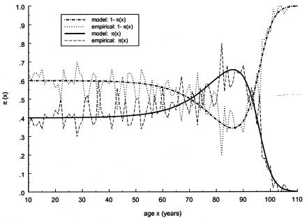We assume that the forces of mortality μ_i(x), i=0,1) for respective genotypes follow the gamma-Gompertz model , where a_i, b_i, and s_i are parameters. Vaupel et al. (1979), Yashin et al. (1994), and Thatcher et al. (1998) have shown that this model fits demographic mortality data better than the traditional Gompertz curve. The graphs of theoretical and empirical proportions in the population of two genotypes are shown in figure 1. Altogether, data for 10,000 individuals (100 individuals for each age, for ages 10 years–110 years) were simulated. One can see that the quality of simulation is sufficient to use these data for testing our estimation methods.

Figure 1.

Age trajectories of frequencies and their empirical estimates, calculated in simulation experiments for genotypes 0 and 1. The gamma-Gompertz model for the mortalities of genotypes used is as follows: , with a₀=4×10^-5, b₀=.1, P=.4, s²₁=s²₂=.3, a₁=4×10^-10, and b₁=.23.

Genetic Data for mtDNA

The genetic data collected in the study of Italian centenarians are shown in table 1. One can find a detailed description of the Italian data in the work of De Benedictis et al. (1998a) and Yashin et al. (1998).

Table 1.

Absolute Frequencies of mtDNA Haplogroups in Individuals of Various Ages Sampled from the Italian Population

	No. In Age Classes
mtDNA Haplogroup	⩽15 Years	16–25 Years	26–35 Years	36–45 Years	46–55 Years	56–65 Years	66–75 Years	⩾100 Years
H	3	16	37	20	14	12	6	85
I	0	0	1	3	0	2	1	8
J	0	0	3	2	3	4	1	23
K	0	4	4	3	2	4	4	15
T	0	4	8	5	4	6	2	18
U	2	4	10	11	9	2	8	26
V	0	1	1	0	0	1	2	11
W	1	2	2	3	1	1	0	3
X	0	0	5	1	0	1	1	8
A	0	3	9	8	0	6	2	15
Total	6	34	80	56	33	39	27	212

The Idea of the GF Method

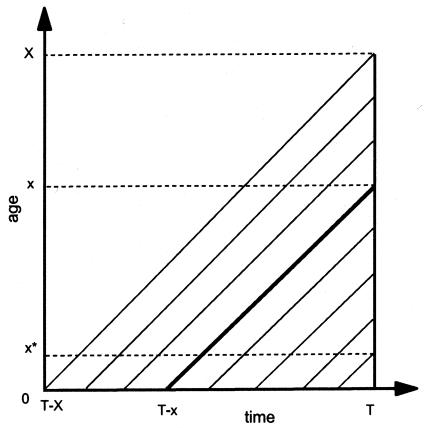
Let T be the year of data collection, x be the age variable, and N_i(x,T-x), i=0,1 be the number of x-year-old individuals carrying the ith genotype observed in the cross-sectional study. Here, x=0,1,…,X, where X is the oldest age represented in the study. The cross-sectional sample represents several cohorts of individuals born in different years, and the argument T-x merely emphasizes the fact that the counted individuals belong to a cohort born in year T-x (see fig. 2). In our estimation procedures, we will consider only two genes or genotypes. The number “0” is associated with the candidate genotype. The number “1” is associated with any other, non-“0” genotype. This method can easily be extended to the case of a population with more genotypes. However, the benefits of such an extension should always be weighed against the loss of power in the estimation procedure, which is the result of an increase in the number of parameters to be estimated.

Figure 2.

Lexis diagram of the difference between cohort and cross-sectional data. The cross-sectional study is performed in year T. The thicker solid line denotes a cohort born in year T-x.

The simplest way to assess the effect of genes on longevity, with use of these data, is to aggregate the sample into two age groups. The “control,” or “younger,” group contains all individuals with age <100 years. These individuals are of two genotypes, 0 and 1, and their numbers are N_iY, i=0,1. The “centenarian” group contains individuals with age ⩾100 years. The numbers of respective genotypes in this group are N_iC, i=0,1. Here, the indices “Y” and “C” denote the control and the centenarian groups, respectively. The empirical estimates of relative frequencies , with i=0,1 and j=Y,C, in these two groups are

These estimates can be used to test the null hypothesis (i.e., that the frequencies of a given genotype are the same in both age groups) against the alternative (i.e., that they are not). This is, in essence, the GF method, as it has been discussed in many publications (e.g., see Proust et al. 1982; Takata et al. 1987; Schächter et al. 1993; De Benedictis et al. 1997). This “model-free” method does not use additional information. However, the use of demographic information about the population under study may substantially improve our understanding of the role of genes in aging and survival.

Demographic Data: Why Are They Helpful?

Let us first consider the cohort study. The benefits of the use of demographic information about marginal survival in the population result from the possibility of the use of the representation for marginal survival function, S(x)—which can be taken from the cohort demographic life tables—as a discrete mixture of the respective survival functions for genotypes. Let us assume that we are dealing with two genotypes 0 and 1, as described above. Let S_i(x) and π_i(x), i=0,1, be the survival functions and frequencies of the respective genotypes, and let π₀(0)=P₀=P and π₁(0)=P₁=1-P be the initial frequencies for the 0 and 1 genotypes, respectively. For simplicity, we will use the notation π(x)=π₀(x) for the frequency of the 0 genotype at age x years and the notation 1-π(x)=π₁(x) for the frequency of genotype 1 at age x years. Then, the relationships between S(x), S_i(x), i=0,1, and π(x) are, according to the method of Vaupel and Yashin (1985), as follows:

and

When functions S(x) and π(x) are known exactly for the age interval (0,X), where X is the maximum age in the study, the initial gene frequency P=π(0) for the 0 genotype is also known, and the survival functions for the two genotypes can be calculated, from equations (1) and (2), as

Thus, when the trajectories for genotype frequencies are known exactly, the addition of demographic information in the form of the marginal survival function solves the problem of determining the genetic influence on survival. One can easily show that this result does not depend on the number of genotypes observed in the study. In reality, proportions of genotypes are not known exactly. The substitution of empirical estimates of π_i(x) and P_i into equation (3) may create problems, since trajectories for the estimates of survival functions for genotypes may become nonmonotone (thus, respective estimates of mortalities could have negative values). In this case, statistical methods are needed to estimate survival characteristics of genotypes.

Merging Demographic Information with Cross-Sectional Data

Genetic data for humans are usually collected in a cross-sectional study, in some year T. If the proportions of genotypes were known exactly, the use of demographic information could solve the problem of genetic influence on survival, in exactly the same way as with the cohort data. Unfortunately, the proportions of genotype 0 at age x, π(x,T-x), are not known exactly. As in the case of the GF method, we assume that π(0,T-x)=P, for all cohorts born in year T-x, with x=0,1,2…,X. Often, the numbers N_i(x,T-x), where i=0,1, are known, beginning with an age of x^* years >0. In this case, one has to assume that π(x^*,T-x)=P^* (i.e., the gene frequencies at age x^* years are the same for all birth cohorts). For the cross-sectional data, equations (1) and (2) can, therefore, be rewritten as

and

The survival function in the left-hand part of equation (4), which can be expressed as

can be taken from a cross-sectional demographic life table for the year T for the respective population, and, hence, it is a known function of x. Note that function characterizes survival in the synthetic (i.e., artificial) cohort, with the mortality . The proportion of individuals, of age x years, carrying candidate genes in the synthetic cohort is Respective survival functions for individuals carrying 0 and 1 genotypes are

with , i=0,1. Empirical estimates can be calculated for each age x=0,1…,X from the numbers N_i(x,T-x), i=0,1 as

Thus, we assume that the data were obtained from binomial sampling with probability of success . As in the cohort case, functions calculated from the analogs of equation (3) with π_i(x) replaced with and S(x) replaced with , do not necessarily decline monotonically, and, hence, they—strictly speaking—cannot be considered as the estimates of , i=1,2 (i.e., estimates of survival functions for genotypes). This is why statistical methods for estimating the survival functions , i=0,1 are needed. In this article, we show that methods that are done on the basis of the maximum-likelihood procedure can be used successfully in the joint analysis of genetic and demographic data to solve this problem.

The Likelihood Function of Genetic Data

The following likelihood function of genetic data is the basis for an estimation procedure, in all of the methods discussed in the sections that follow:

Here, N₀(x,T-x) and N₁(x,T-x), x=x^*, x^*+1,…X, are the number of individuals with and without the genotype 0, respectively, aged x years at time T. Since we identify π(x,T-x) with π(x), which satisfies equation (5), the likelihood function becomes

The parameter P, as well as the two survival functions , i=0,1 for genotypes, are unknown. Their values at each age x years have to be estimated on the basis of the available data. Altogether, 2(X-x^*)+1 parameters have to be estimated (i.e., X-x^* parameters for each of the two survival functions, plus P.) Note that here we assume that S_i(x^*)=1, i=0,1.

Demographic, Epidemiological, and Other Constraints

One cannot estimate the initial frequency P and the two survival functions , i=0,1, by maximizing equation (7) without additional conditions, since this model is nonidentifiable. The demographic condition of equation (4), where is known, allows us to reduce the number of model parameters to X-x^*+1, since equation (4) includes X-x^* conditions (one for each age). Simulation studies show that these parameters are identifiable. Thus, the likelihood function of equation (7) has to be maximized with use of equation (4). Sometimes, additional conditions can stem from the results of epidemiological studies in which the values of relative risks r(x), for respective genotypes, are estimated at some selected age interval. For example, the ratio of hazards for two genotypes,

may be known for x=x₁,x₂,…,x_n. In this case, the likelihood function of equation (8) has to be maximized with use of constraints in equations (4) and (9). Hence, the number of model parameters becomes X-x^*-n+1. When the sample size of genetic data is large enough, the NP method may provide acceptable estimates for survival functions , i=0,1 of genotypes and for P.

The NP Method

The NP method allows us to estimate X-x^* values of function , without any assumptions about its parametric form (that is why we call it the “NP method”), and to estimate P for genotype 0. For these purposes, it is better to represent in terms of conditional probabilities of death q⁰_x (i.e., the probability that death will happen at the interval between x and x+1, given that it did not happen until age x years). Thus, can be represented as The estimation can be made with the maximization of equation (8) under the demographic constraint of equation (5), with respect to parameters q⁰_y, y=x^*, x^*+1,…,X and P,0⩽q⁰_y⩽1; 0⩽P⩽1. When and P are estimated, the survival function for genotype 1 is calculated from equation (4). These estimates can be obtained even without the additional information provided by equation (9), when the sample size of genetic data is large enough.

When the sample size of the data is small, the NP estimates may be unreliable. In this case, additional conditions that reduce the number of estimated parameters may improve the power of the estimates. In this article, we consider three kinds of such conditions. The first condition assumes proportionality among hazards associated with respective genes or genotypes (the RR method). The second condition assumes that the survival functions of genotypes , i=0,1 are of a specific parametric form (the PR method). The third condition assumes parametric form for only one survival function, say for . The other survival function, , is calculated with the SP method.

The RR Method

This method assumes that μ₁(x,T-x)=zμ₀(x,T-x), x=x^*, x^*+1,…,X, which implies

Here, hazards and are associated with survival functions and , respectively. Parameter z is the unknown relative risk associated with the genotypes collectively labeled as “1.” If z>1, then individuals carrying the 0 genotype have a survival advantage, and the genotype is called a “robust genotype.” If z<1, then the situation is reversed, and 0 is a “frailty genotype.” Under this assumption, function in equations (8) and (4) must be replaced by . Let us assume that function in equation (4) is known (i.e., demographic information is available). Then, conditions in equations (4) and (10) leave only two unknown parameters, z and P. Equation (9) reduces the problem to the estimation of parameter P only. When the estimates of z and P are known, , x=x^*+1,…,X can be calculated from equation (4).

The parameter estimates can be obtained by the method of constraint likelihood maximization or by an algorithm that involves the repetition of the following steps. Make an initial guess of ) and solve the maximum-likelihood problem for parameters P⁽⁰⁾ and z⁽⁰⁾ by use of equations (8) and (10). Then, calculate from equations (4) and (10) for the given parameters P⁽⁰⁾ and z⁽⁰⁾. Take as the next guess and calculate P⁽¹⁾ and z⁽¹⁾ by use of equations (8) and (10), and so forth. Our simulation studies show that this procedure converges with the maximum-likelihood estimates of parameters z and P. This procedure can be easily extended when data are available for observed covariates (e.g., location and sex) (Yashin et al. 1998).

The PR Method

In the PR method, survival functions , i=0,1 are described parametrically. Such a specification reduces the number of model parameters. For example, one can assume that the force of mortality for genotype i follows the Gompertz-Makeham curve:

Here, parameters c_i, a_i, and b_i characterize the survival functions of genotype i, i=0,1, in the data from a cross-sectional study. In the case of specification (11), one has to estimate seven parameters. Such estimates can be obtained by use of the constraint maximum-likelihood method—that is, by maximization of equation (8) with constraints (4) and (11), with consideration given to the fact that

Other estimation procedures can also be suggested. For example, the constraint LSPR method can be considered as an alternative to the maximum-likelihood procedure. A version of such a method with an ad hoc procedure for consideration given to constraints was used by Toupance et al. (1998). The benefits and limitations of these methods are reviewed in the Discussion.

The SP Method

To minimize the number of technical assumptions about the parametric structure of the survival curves for genotypes, one can assume that only one survival function—say, —is described parametrically. For example, one can assume that the force of mortality for genotype 0 follows the Gompertz-Makeham curve (equation [11]) specified for i=0. Here, parameters c₀, a₀, and b₀ characterize the survival functions of genotype 0 in a cross-sectional study. When parametric specification for is chosen, and if the marginal survival function is known, then can be derived from equation (4), as a function of parameters c₀, a₀, b₀, and P. This function must be substituted into the likelihood function given in equation (8). After that, direct maximization of equation (8) gives the estimates of parameters c₀, a₀, b₀, and P. Now, the estimates of survival characteristics for respective genotypes can be easily calculated. Note that, for some values of the parameters, the function —calculated as —may be a nonmonotone function of x and, hence, cannot be used, in the likelihood function (8), as a survival function. In this case, one must approximate by an appropriate survival function. For example, one can use survival function , such that , if , and , if . Such a precaution must accompany any method using equation (4) to calculate .

Consideration of Population Heterogeneity

The fact that heterogeneity in mortality may bias the results of survival analyses when its possible presence is ignored in the estimation algorithm is well known (Vaupel et al. 1979; Vaupel and Yashin 1985). The use of the NP method, which estimates the respective q⁰_x, x=x^*, x^*+1,…,X, is the most flexible way to control for the presence of heterogeneity. To correct for heterogeneity in the RR method, we use the gamma-frailty model (Vaupel et al. 1979) for a population of individuals with genotype 1. In accordance with this model, μ₁(x)=Yzμ₀(x), where the random variable Y is gamma distributed with mean 1 and variance σ². In this case,

and, in addition to z and P, one has to estimate parameter σ². The respective estimation procedure is called the “HRR method.”

In the case of the PR method, heterogeneity is taken into account with use of gamma-Gompertz mortality models (Yashin et al. 1994) for genotypes, instead of with use of traditional Gompertz or Gompertz-Makeham curves. An alternative model assumes that this force of mortality follows the logistic gamma-Makeham curve (Yashin et al. 1994).

Specification (12) requires the estimation of nine parameters; a_i, b_i, c_i, and s_i (i=0,1); and P. To control for heterogeneity in the SP method, it is enough to assume that the survival function is characterized by the mortality rate in equation (12) (when i=0).

Results

Applications to Simulated Data

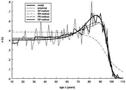
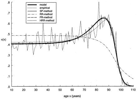
To test the approaches described in the preceding sections, we first applied them to simulated data. The graphs of empirical and estimated proportions for genotype 0 are shown in figure 3. Here, the estimates for the PR and SP methods were obtained with use of Gompertz's parametrization of respective mortality curves. (Note that the data were simulated with the gamma-Gompertz mortality curve). One can see that the PR and SP methods give a better fit to the data than does the RR method. Figure 4 shows similar estimates, obtained with the gamma-Gompertz specification of respective mortality curves. Such a specification allows us to control for unobserved heterogeneity in mortality. One can see that the quality of estimation with the SP and PR methods improves when unobserved heterogeneity is taken into account. Use of the HRR method results in the estimation σ²=0. So, the HRR estimates coincide with the RR estimates, for this example.

Figure 3.

Age trajectories of gene frequencies for the 0 genotype, obtained in simulation experiments. These include simulated trajectories (denoted by a thick solid line) and their empirical estimate (denoted by a short dashed line), as well as estimates obtained by the NP method (denoted by a medium solid line), the SP method, (denoted by a thin solid line), the RR method (denoted by a dashed-dotted line), and the PR method (denoted by a long dashed line). The PR and SP methods were done with use of the Gompertz parametrization of mortality curve for the 0 genotype, as follows: μ₀(x)=a₀e^b₀x.

Figure 4.

Age trajectories of gene frequencies for the 0 genotype, obtained in simulation experiments. These include simulated trajectories (denoted by a thick solid line) and their empirical estimate (denoted by a short dashed line), as well as estimates obtained by the SP method (denoted by a thin solid line), the RR method (denoted by a dashed dotted line), the PR method (denoted by a long dashed line), and the HRR method (denoted by a thin short-dashed line). The PR and SP methods use the gamma-Gompertz specification of mortality curve for the 0 genotype, as follows: .

Application to Data on Haplotypes of mtDNA

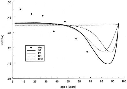
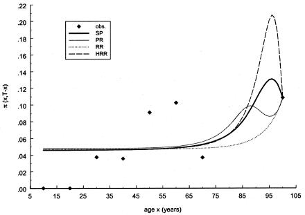
Table 2 shows the results of an analysis of Italian data for mtDNA haplogroups H and J, with use of the RR method. To obtain a 95% confidence interval (CI) for the estimate of the frailty parameter, 100 bootstrap replicates (Weir 1996, p. 53) of each age class were generated, and the corresponding values for P and z were estimated for the H and J haplogroups. The estimated values for z show that haplogroup H clearly has no effect on survival, whereas haplogroup J has a significant positive effect. A similar result concerning haplogroups J and H was obtained previously by Yashin et al. (1998), who used a smaller data sample. Figures 5 and 6 show the observed relative frequencies, together with the age trajectories of the frequencies, computed with the estimates obtained with the RR method (denoted by a dotted line). Note that the trajectories interpolate exactly the empirical frequencies of the sample of centenarians, the size of which is much larger than the size of the samples of younger ages.

Table 2.

Estimates of P and z for mtDNA Haplogroups J and H

Haplogroup	P Estimate	z Estimate (95% CI)
J	.04	1.19 (1.05–1.37)
H	.39	1.00 (.97–1.04)

Figure 5.

Observed frequencies of mtDNA haplogroup H (denoted by blackened diamonds) in a sample of Italian data, together with estimated cross-sectional age trajectories obtained with the SP method (denoted by a thick solid line), the PR method (denoted by a thin solid line), the RR method (denoted by a dotted line), and the HRR method (denoted by a dashed line). The PR and SP methods use the gamma-Gompertz specification of mortality curve for the 0 genotype.

Figure 6.

Observed frequencies of mtDNA haplogroup J (denoted by blackened diamonds) in a sample of Italian data, together with estimated cross-sectional age trajectories obtained with the SP method (denoted by a thick solid line), the PR method (denoted by a thin solid line), the RR method (denoted by a dotted line), and the HRR method (denoted by a dashed line). The PR and SP methods use the gamma-Gompertz specification of mortality curve for the 0 genotype.

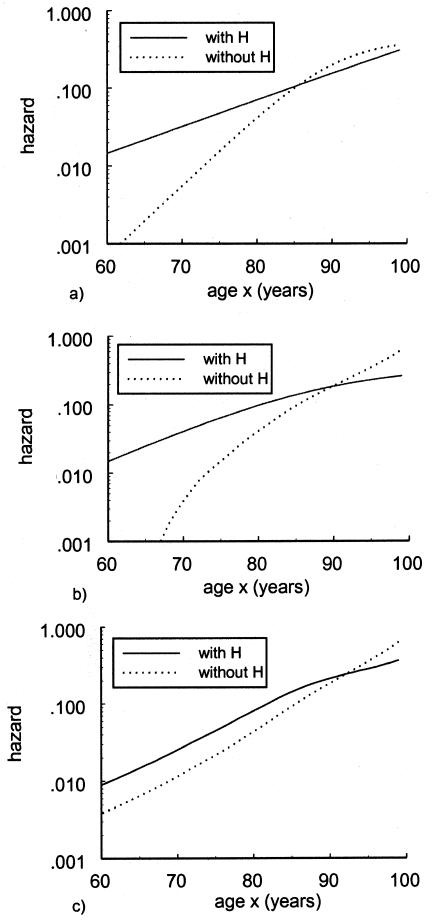
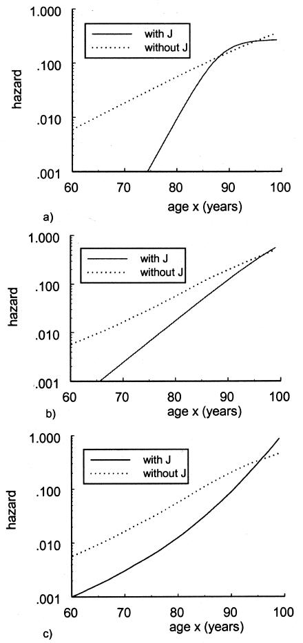
It should be noted that the NP estimates are not shown in these graphs because the use of this method requires a larger sample size of the data. The PR and SP methods, described in respective sections, were tested with the same data. Figures 5 and 6 show the age trajectories of frequencies for respective haplogroups (denoted by thin solid and thick solid lines, respectively). Clearly, these methods produce nonmonotonic trajectories of gene frequencies. Such trajectories correspond to the haplogroups with intersecting hazard rates for haplogroup H (fig. 7) and haplogroup J (fig. 8). Figure 7 shows the logarithms of the age trajectories of hazards for haplogroup H (denoted by a solid line) and for the rest of the population (denoted by a dotted line). Figure 8 shows similar graphs for haplogroup J. Note that, in the case of parametric hazards, the classification of genotypes into “robust,” “frail,” and “neutral” categories is not necessary, since the entire trajectories of the hazards are estimated.

Figure 7.

Logarithms of mortalities for individuals with mtDNA haplotype H (denoted by a thick solid line) and without haplotype H (denoted by a dotted line). Estimates are made with use of the PR method, the SR method, and the HRR method.

Figure 8.

Logarithms of mortalities for individuals with mtDNA haplotype J (denoted by a thick solid line) and without haplotype J (denoted by a dotted line). Estimates are made with use of the PR method, the SR method, and the HRR method.

Sensitivity Analysis

In this section, we investigate the effects of violation of assumptions i and ii, discussed in the Introduction. For this purpose, we assume that mortalities for two different genotypes are related by the proportionality condition. The empirical justification for such an assumption is made on the basis of the results of Yashin et al. (1998), in which the use of the proportional-hazards assumption in the RR method, applied to Italian data on genetic markers, confirmed earlier findings obtained with the traditional GF method. Theoretical justification of the proportional–hazards model have been discussed by Yakovlev et al. (1995). Their results suggest that relative risk may be considered as a measure of the vulnerability, of respective genotypes, to the process of lesion formation associated with aging. Other applications of this model have been discussed by Cox and Oakes (1984). Space limitations do not allow us to perform similar analyses of the other models discussed in this article. The goals of the present sensitivity analysis are to investigate the following:

• 1. to what extent π(x,T-x) depends on the parameter z, for the fixed and time-independent initial frequency of the genotype π(0,t)=P, and on survival functions for genotypes, independent of the birth year of the cohort (assumptions i and ii hold);
• 2. to what extent does π(x,T-x) depend on a variable initial frequency π(0,t), for a fixed z>1 (assumption ii holds);
• 3. to what extent does π(x,T-x) depend on changes in a survival of the genotypes for different cohorts, when π(0,t)=P (assumption i holds) and z is constant; and
• 4. to what extent does π(x,T-x) depend on a possible change in z of the birth year of the cohort, when π(0,t)=P (assumption i holds).

To perform this analysis, we first selected survival function , which we call the “reference” survival function. To make our analysis more realistic, we constructed by using life-table data for the Italian population, taken at the end of the 19th century (Del Panta and Rettaroli 1994). To model the improvement in survival, we used the model , in which a(t) declined linearly, from 1 to .3, over a time of 105 years. Here, a(T)=1-[.7/105(t-t₀)]. We assume that life expectancy in the youngest cohort is ∼85 years, which corresponds to a(t)=.3. The cohort with the survival function is characterized as a “young” cohort. Note that the survival function S_y(x) is hypothetical, and future mortality for the youngest cohort in the study is unknown. 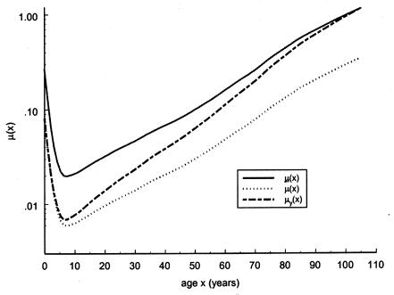We then used , , and S_y(x) to model survival functions for genotypes in the old (i.e., subjects who were born in some year t₀ in the past), intermediate (i.e., subjects who were born in the year t, t₀<t<t₀+105), and young (i.e., subjects were born in the year t₀+105) cohorts, respectively. 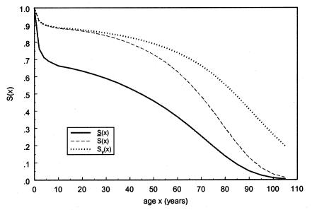Figure 9 shows graphs for three mortalities, , μ_y(x)=μ(x,t₀+105), and μ(x,t₀+105-x), where μ(x,t₀+105-x) is the mortality, in the synthetic cohort, corresponding to hypothetical cross-sectional data. Figure 10 shows the graph of the survival function in the synthetic cohort S₀(x), corresponding to the year T=t₀+105, along with graphs of two cohort survival functions, and . One can see that the function appears to be different from the respective cohort functions. Note that if assumptions i and ii hold, then functions and S(x,T-x) coincide. However, in the presence of secular trends in mortality, . In general, S(x,T-x) is not a survival function because it can be a nonmonotone function of age.

Figure 9.

Logarithms of three mortality rates: mortality μ(x) (denoted by a solid line), in the cohort of Italian females born at the end of the 19th century (Del Panta and Rettaroli 1994); mortality (denoted by a dotted line), in the hypothetical “young” cohort; and mortality (denoted by a dashed line) in the synthetic cohort constructed from cross-sectional data. μ(x) and μ_y(x) are used as baseline mortalities in a sensitivity analysis.

Figure 10.

Survival functions for genotype 0: in the old cohort, (denoted by a solid line); in the hypothetical young cohort, S₀(x)=S_y(x)(denoted by a dotted line); and, in the synthetic cohort constructed from cross-sectional data, (denoted by a dashed line).

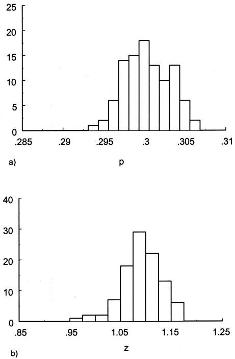
To investigate the effects of risk parameters and initial frequencies on age trajectories of the proportions of genotype, we will consider two hypothetical subpopulations (one consisting of individuals carrying a given genotype 0, and the other—population 1—consisting of individuals without the genotype). We used the RR model for the cohort born in year t₀, with and S₁(x,t₀)=S₀(x,t₀)^z and then with S₀(x,t₀)=S_y(x) and S₁(x,t₀)=S_y(x,t₀)^z. Here, S₀(x,t₀) and S₁(x,t₀) are cohort survival functions for the respective genotypes, and z is the value of the relative risk. The cross-sectional trajectories of the proportion of genotype 0—again denoted by π(x,T-x)—were computed with equation (3), with π(0,t)=P for all t₀⩽t⩽T. Figure 11 shows the histograms of parameter estimates, obtained in 100 simulations of genetic data for 10,500 individuals (assumptions i and ii hold). The true values of these parameters are P=.3 and z=1.1. 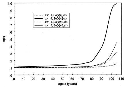The survival functions are and . The marginal survival function was taken to be S(x)=PS₀(x)+(1-P)S₀(x)^z. Figure 12 shows how the cross-sectional trajectory of genotype frequency π(x,T-x) depends on parameter z, in the absence of secular trends, in the survival of a cohort (assumptions i and ii hold). In this case, π(x,T-x) coincides with the age trajectory of the genotype proportion in any cohort. The experiments were done for two values of relative risk, z=1.1 and z=1.5 (thus, genotype 0 is robust), with either survival function or S₀(x)=S_y(x). The initial frequency chosen was P=.1. It is obvious that π(x,T-x) should increase with age x. The interesting point here is that the most relevant change in frequency occurs in very old cohorts; this result justifies the relevance of studying groups of centenarians. Moreover, the high mortality among both genotypes, which occurs when , enhances the effect of “robustness” on the gene frequency. The presence of hidden heterogeneity in mortality for genotypes can mask this effect.

Figure 11.

Histograms of estimates of initial frequencies P (a) and relative risk z (b), obtained from simulated data (10,500 individuals and 100 samples), with the RR method. The true values of these parameters are P=.3, z=1.1, , and S(x)=PS₀(x)+(1-P)S₀(x)^z.

Figure 12.

Age trajectories of the relative frequency of genotype 0 (the robust genotype), under assumptions i and ii. The trajectories are reported for various values of the parameter z >1 (RR model) and for different baseline survival functions, as follows: z=1.1, (denoted by a dashed line), z=1.1, S₀(x)=S_y(x) (denoted by a dotted line), z=1.5, (denoted by a thick solid line), and z=1.5, S₀(x)=S_y(x) (denoted by a thin solid line).

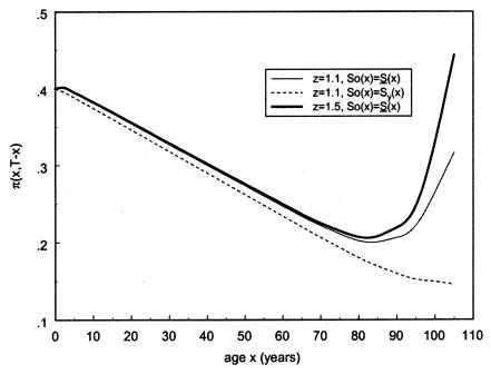
Let us now analyze the effect of a change in initial frequency of genotype 0 (assumed to be robust—i.e., with z>1) in the birth cohorts in a cross-sectional trajectory of gene frequency π(x,T-x). If the initial frequency π(0,t) in the cohort born in year t decreases with time, then the rate of increase in frequency observed in a cross-sectional trajectory is obviously enhanced. However, if π(0,t) increases with time, then the frequency π(x,T-x), measured in a cross-sectional study, can decrease, at least when z=∼1. This last case is shown in figure 13, in which it is assumed that π(0,t) varies linearly, from .1 for t=t₀ (i.e., for the cohort of people of age 105 years in the cross-sectional sample) to .4 for t=t₀+105 (i.e., the cohort of newborns in the cross-sectional sample). Such a rate of change in the initial frequency is purely hypothetical; however, the simulation shows that, if it had occurred in a real population, and if the data drawn from a cross-sectional sample of age 10–70 years were analyzed by simply comparing genotype frequencies in different age classes, then the genotype would have been classified as a frailty genotype. This example shows that possible changes in the initial proportions must be carefully controlled, because they may seriously bias the results of standard analysis of gene frequencies or may even mask completely the effect of a favorable gene.

Figure 13.

Effect of an increase in the initial frequency of the robust genotype 0 with the birth year of the cohort, under assumption ii. The graphs show the cross-sectional trajectories of genotype frequencies for various values of the parameter z (RR model) and the different baseline survival functions, as follows: z=1.5, (denoted by a thick solid line); z=1.1, (denoted by a thin solid line); and z=1.1, S₀(x)=S_y(x) (denoted by a dashed line). It is assumed that π(0,t) increases linearly, from .1 for t=t₀ (i.e., for the cohort of people of age 105 years, in the cross-sectional sample) to .4 for t=t₀+105 (i.e., the cohort of newborns in the cross-sectional sample).

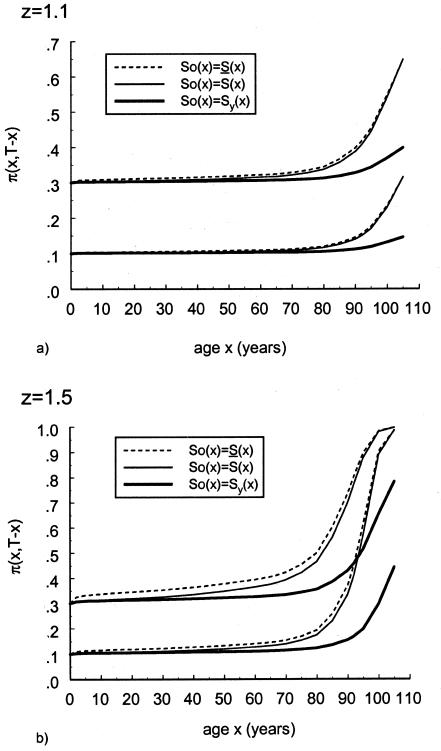
Figure 14 shows the results of the numerical experiments aimed at investigating the extent to which the cross-sectional trajectory π(x,T-x) depends on changes in the survival of different cohorts, when the initial frequency is kept constant (assumption i). Since z>1, genotype 0 is robust; as expected, the cross-sectional trajectory of this genotype lies between the “longitudinal” trajectories that would be obtained with use of the survival functions pertaining to the oldest and the youngest cohorts. It is clear that the differences between the trajectories increase for the larger values of z. However, since the main effect of the presence of a robust and of a frail subpopulation is seen in populations with older ages, the demographic characteristics of older cohorts strongly influence the cross-sectional trajectory.

Figure 14.

Comparison of cross-sectional and longitudinal trajectories of the frequency of genotype 0, when secular trends in the survival functions occur. Longitudinal trajectories are shown for (denoted by a short dashed line) and S₀(x)=S_y(x) (denoted by a thick solid line). The cross-sectional trajectories (denoted by a thin solid line) were computed under the assumption that the survival function changed, from for the oldest cohort to S₀(x)=S_y(x) for the youngest cohort. Initial frequencies are assumed to be independent of the year of birth and are given either as P=.1 or P=.3. Panels a and b correspond to z=1.1 and z=1.5, respectively.

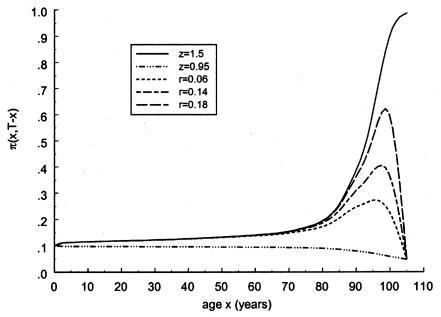
To analyze the effect of a variable risk, z was assumed to decline with t—for example, from the oldest cohort (with birth year t=t₀) to the youngest cohort (with birth year t of T=t₀+105)—in accordance with the exponential law

with z₁=1.5 and z₂=0.95 for several values of parameter r. The effects of a change in the risk z, with the birth year t of the cohort, are shown in figure 15.

Figure 15.

Age trajectories of gene frequencies in a hypothetical cross-sectional study, when S₁(x,t)=S₀(x)^z(t) and , with z(t)=(z₂-z₁)exp[-r(105-t)]+z₁, for z₁=1.5, z₂=0.95 r=.06, r=.14, and r=.18. For comparison, the cohort trajectories of gene frequencies corresponding to survival function with z=1.5 (denoted by a solid line) and z=0.95 (denoted by a dashed dotted line) are also shown.

One can see that, with this model, the change in z causes nonmonotonic cross-sectional trajectories of the genotype frequency. In particular, this example shows that a comparison of genotype frequencies for only two age groups (the group of the 80-year-old subjects and the group of centenarians) may not help in the detection of genetic effects.

Discussion

The present study shows the benefits of combining genetic methods and data with the methods and data of demography, epidemiology, and biostatistics, to address questions concerning the genetic nature of the human life span. Although relatively simple hypotheses about the presence and type of genetic influence on survival can be tested by use of the traditional GF method, results obtained with this method often do not satisfy researchers interested in more-fundamental aspects of this influence. For example, the age-specific hazard rates, survival functions, or values of relative risks for respective genes or genotypes give us more information about the roles of genes in aging and life span than is provided by just the classification of genes as robust, frail, or neutral. To estimate these characteristics, additional data and more-sophisticated models are required. Which data and which models have to be used?

For humans, genetic data usually come from cross-sectional (not cohort) studies, and, hence, gene frequencies are compared among individuals from different cohorts. For this reason, demographic aspects of aging and survival in populations with different birth cohorts must be taken into account in the analysis of data on genetic markers. It turns out that the use of demographic and epidemiological information, together with genetic data, may substantially improve the results of such an analysis. Demographic data are now widely available and can be accessed easily. Also, the range of available epidemiological data is rapidly increasing. Development of methods that combine demographic, epidemiological, and genetic information will enhance our ability to investigate complicated problems of aging and longevity. With more information and richer data, more characteristics of genetic influence on survival can be evaluated. All the new methods described in this article allow us to estimate survival and hazard functions for genotypes. Such estimates cannot be obtained with the GF method and use of genetic data alone.

The methods discussed in this article are based on the maximum likelihood–estimation procedure. This allows us to test statistical hypotheses about the functional form of hazard functions, by using the likelihood-ratio test. Since the role of candidate genes in the human life span can be masked by the effects of other genes and unobserved environmental factors, methods capable of controlling for hidden heterogeneity in mortality are needed (Vaupel et al. 1979; Vaupel and Yashin 1985). We show that all of the methods discussed in this article can be adjusted to control for hidden heterogeneity. When demographic or epidemiological data are used, instead of marginal survival or risk functions r(x)=μ₀(x)/μ₁(x), the respective likelihood functions of these data must be included in the joint likelihood function, which we have to maximize.

The GF method can control for the effects of other, nongenetic factors on survival that are measured in cross-sectional studies (i.e., location and sex). However, use of this method requires stratification of the available data (i.e., by location or sex). This stratification requirement may substantially reduce the power of the estimation procedure, since the sample sizes of the data, in each stratum, may become small. For this same reason, it would be difficult to address questions about the effects of interaction of nongenetic factors on candidate genes by use of the GF method. The use of aggregated data, with the inevitable loss of information, is another weakness of the GF method.

The proportional-hazards model for genotypes that is used in the RR method may capture major differences in the survival of genotypes when respective hazard curves do not intersect. The idea of proportionality of hazards, which was suggested by Cox (1972), has been widely used in demography, epidemiology, and biostatistics (e.g., see Vaupel et al. 1979; Cox and Oakes 1984; Clayton and Cuzick 1985). The use of this method is justified when one is satisfied with approximating hazards for genotypes by using the values of relative risks multiplied by the underlying hazard. This model may also be viewed as a linear approximation of the nonlinear hazard μ(x,z), where z characterizes differences between genotypes. Recent development and applications of this approach have been discussed by Andersen et al. (1992). When real hazard rates for genotypes intersect, the estimates of these hazards, obtained by the RR method, reflect the “average” results of complicated selection mechanisms, which depend on the behavior of respective hazard curves. For example, if there is only one point of intersection—and if it occurs at a very young or at a very old age—then the proportional hazards calculated by the RR method can still represent the average effects of selection mechanisms in the population. In other cases, important details related to age trajectories of hazards may be missed. For this reason, the use of several approaches provides a comprehensive analysis of the gene-frequency data and helps us to better understand the regularities of gene-environment interaction at different stages of the individual aging process.

A simplified version of the PR method, which is modeled on the basis of the minimum LSPR method, has been used by Toupance et al. (1998) to investigate the survival of genotypes in the ACE locus. In their article, Toupance and colleagues modeled the hazards for three genotypes by means of Gompertz-Makeham curves. Note that, instead of the maximum-likelihood method, Toupance et al. (1998) used the constraint LSPR method with an ad hoc procedure for taking into account constraints. They aggregate the empirical frequencies of candidate genotypes in two groups—a group of centenarians and a group of younger individuals—and use them as the constraints in the method. An additional constraint—the risk ratio for respective genotypes, estimated earlier in a separate study—has also been used.

Such an estimation strategy does not allow us to test the fitness of different models or the similarity of hazards for genotypes. The aggregation of gene frequencies in the two age groups produces an inevitable loss of information, which may bias the parameter estimates. Furthermore, the aggregation reduces the power of the estimation procedure and may lead to erroneous conclusions about the role of genes in mortality and longevity. We must note, however, that most of these limitations can be eliminated, and the method is certainly a step forward from the traditional GF-method approach to the analysis of gene-frequency data.

The simulation experiments with parametric models done in our study confirm the importance of measuring the relative proportions of genotypes in several age groups of individuals. Such measurements may reveal that the dynamics of gene frequencies are nonmonotone, which often results in crossovers of the age-specific hazard rates associated with respective genotypes. Note that, in the case of the SP method, there is no need to give a parametric description to survival functions corresponding to all genotypes; at least one survival function can be estimated semiparametrically. This adds more flexibility to the analysis of genetic data and may increase the power of the estimation procedure.

The new methods discussed in this article require the same assumptions concerning initial gene frequencies in different birth cohorts (assumption i). Although meaningful changes in such frequencies, as a result of evolutionary developments, are unlikely in the time considered, the contribution of migration flows may be significant for some populations. When not properly treated, the presence of such migration may bias the results of comparison of gene frequencies in a cross-sectional study. Thus, analysis of historic demographic data should accompany such genetic studies, to avoid this potential bias. In particular, the selection of individuals for the sample should take into account the demographic history of the families, to eliminate the problem at the early stage of data collection.

Unfortunately, there is no exact answer to the question about the best method. All of the new methods discussed in the present article provide us with more information about survival of genotypes than does the traditional GP method. The NP method is the most flexible but requires a large sample size of the data. The SP method requires parametric description of one hazard rate, but it is a good choice when some additional information justifying such a parametric structure is available. The PR method requires more ancillary information to justify parametric structure of the respective genotypes. The RR method is the simplest: it involves only two unknown parameters, but the assumption of the proportionality of hazard does not allow investigators to capture the intersection of the hazard rates for genotypes when such an intersection exists. The correction for heterogeneity adds more flexibility to all the methods. The GF, SP, and PR methods do not allow us to test whether the candidate gene is recessive or dominant. However, such testing can easily be done in the version of the RR method discussed by Yashin et al. (1998).

Note that all of the methods discussed in this article do not take into account the presence of secular trends in mortality. Such estimation strategies cannot be reliable. Industrial progress, improvements in nutrition and living conditions, changes in lifestyle, and other transformations in the human environment may have different survival effects on individuals with different genotypes. A more detailed study of the mechanisms of such gene-environment interactions may require information about risk factors, indicators of socioeconomic development, and cause-specific mortality. For such an analysis, more-sophisticated models of human mortality and aging are needed.

The sensitivity analysis performed in this article allows us to conclude that the major changes in the frequency of genotypes occur at age >80 years (fig. 12), if we assume the proportionality of hazards for genotypes and if the range of relative risk is 1.1–1.5. This situation justifies the practice of collecting genetic data from centenarians and the use of the GF method in the genetic analysis of longevity. The present analysis also shows that changes in the initial frequency of a selected genotype with the birth year of the cohort (i.e., as a result of migration) may seriously disturb the results of analysis, especially when these changes occur rapidly (fig. 13). Whether the effects of secular trends in mortality decline in the proportions of genotypes observed in cross-sectional studies depends on the mechanisms of gene-environment interaction that determine a given trend. Since information about such interactions is not available, we have considered the effects of several hypothetical interaction mechanisms on the age trajectories of gene frequencies. Our analysis shows that these effects are small when mortality declines proportionally for all genotypes (i.e., when relative risk z is constant for all generations) (fig. 14). The effects may be large when mortality decline is associated with one genotype (as in figure 15, in which z changes from 1.5 to 0.95).

Perhaps the most paradoxical finding from the centenarian studies is that survival to age ⩾100 years is not necessarily related to the presence of robust genes (i.e., genes that provide the person with a survival advantage throughout the entire life span), as has been believed previously. The intersection of hazard rates for genotypes, observed in centenarian studies, indicates that the nature of longer survival may be more complicated. Toupance et al. (1998) have associated such intersection with “pleiotropic” effects. Such an explanation involves Williams's (1957) “antagonistic pleiotropy” theory of aging. Under this theory, genes that have beneficial effects on fitness earlier in life may have deleterious effects at later ages. Since the fitness of a genotype involves not only survival but also fertility, it is clear that mortality and fertility should be studied together in models that are established on the basis of evolutionary principles. A summary of the current knowledge of evolutionary theory relevant to the joint analysis of these two important life-history traits has been presented by Charlesworth (1994). The evolutionary consideration allows us to conclude that intersection of hazard rates for genotypes at late ages (i.e., at age >80 years), observed in centenarian studies, may have nothing to do with pleiotropic effects: evolutionary-based intersections must happen at the ages at which evolutionary pressure on fitness is still significant (i.e., at the reproductive interval). Thus, the observed effects must have a different explanation.

One such explanation deals with adaptation of individuals to environmental impacts. The survival advantage may be either lost or acquired in a continuous struggle with the challenges and stresses of life. Curiously, during this struggle, genes that induce higher frailty at the beginning or middle of life may become beneficial at advanced ages. As a result, the hazard rates for populations of individuals carrying different genotypes may cross over. One may expect that the same stress load experienced by individuals in a genetically heterogeneous population will produce different effects in individuals with different genotypes. It is likely that individuals with frail genotypes experience higher pressure on their physiological regulatory systems and homeostatic mechanisms for dealing with the consequences of stresses and environmental insults than do those individuals with robust genotypes. In the long run, the adaptation mechanisms of frail individuals who survive to old age become better “trained” and, hence, better prepared for the inevitable stresses of aging than do those with initially beneficial genotypes. This gene-environment interaction may illustrate the fundamental property of a living organism to develop and maintain the ability to adapt to changes in the internal or external environment and to compensate for losses with homeostatic reserves. If such genetically different adaptation mechanisms are at work, then the candidate genes have to be searched for among those genes that produce survival disadvantage earlier in life. Another reason for the intersection of mortality curves of genotypes may be associated with hidden heterogeneity in mortality (Vaupel et al. 1979; Vaupel and Yashin 1985). This heterogeneity may depend on other genes, which are not considered in a centenarian study.

An interesting question concerning the variety of risks and hazards estimated for different genotypes is: Why are genotypes with higher regular mortalities not eliminated from the population by evolutionary forces? Fisher's “fundamental theorem of natural selection” (Fisher 1930), augmented by the later results of Kimura (1958) and other population geneticists, may help us to better understand the causes generating a variety of survival curves for different genotypes in a population.

References

- Andersen PK, Borgan O, Gill R, Keiding N (1992) Statistical models based on counting processes. Springer-Verlag, New York, Berlin [Google Scholar]
- Aptech Systems (1996) GAUSS: mathematical and statistical system. Vol I: System and graphics manual. Aptech Systems, Maple Valley, WA [Google Scholar]
- Charlesworth B (1994) Evolution in age-structured populations. Cambridge University Press, Cambridge [Google Scholar]
- Clayton DG, Cuzick J (1985) Multivariate generalizations of the proportional hazards model (with discussion). J R Stat Soc A 148:82–117 [Google Scholar]
- Cox DR (1972) Regression models and life-tables (with discussion). J R Stat Soc B 34:187–220 [Google Scholar]
- Cox DR, Oakes D (1984) Analysis of survival data. Chapman & Hall, London [Google Scholar]
- De Benedictis G, Carotenuto L, Carrieri G, De Luca M, Falcone E, Rose G, Cavalcanti C (1998a) Gene/longevity association studies at four autosomal loci (REN, THO, PARP, SOD2). Eur J Hum Genet 6:534–541 [DOI] [PubMed]
- De Benedictis G, Carotenuto L, Carrieri G, DeLuca M, Falcone E, Rose G, Yashin AI, et al (1998b) Age-related changes of the 3′APOB VNTR genotype pool in ageing cohorts. Ann Hum Genet 62:115–122 [DOI] [PubMed]
- De Benedictis G, Falcone E, Rose G, Ruffolo R, Spadafora P, Baggio G, Bertolini S, et al (1997) DNA multiallelic systems reveal gene/longevity associations not detected by diallelic systems: the APOB locus. J Hum Genet 99:312–318 [DOI] [PubMed] [Google Scholar]
- Del Panta L, Rettaroli R (1994) Introduzione alla demografia storica. Editori Laterza, Rome, Bari [Google Scholar]
- Fisher RA (1930) The genetic theory of natural selection. Clarendon Press, Oxford [Google Scholar]
- Hanselman DC, Littlefield D (1998) Mastering MATLAB version 5: a comprehensive tutorial and reference. Prentice-Hall, Upper Saddle River, NJ [Google Scholar]
- Ivanova R, Henon N, Lepage V, Charron D, Vicaut E, Schächter F (1998) HLA-DR alleles display sex-dependent effects on survival and discriminate between individual and familial longevity. Hum Mol Genet 7:187–194 [DOI] [PubMed]
- Kimura M (1958) On the change of population fitness by natural selection. Heredity 12:145–167 [Google Scholar]
- Proust J, Moulias R, Fumeron F, Bekkhoucha F, Busson M, Schmid M, Hors J (1982) HLA and longevity. Tissue Antigens 19:168–173 [DOI] [PubMed]
- Takata H, Suzuki M, Ishii T, Sekiguchi S, Iri H (1987) Influence of major histocompatibility complex region genes on human longevity among Okinawan-Japanese centenarians and nonagenarians. Lancet 2:824–826 [DOI] [PubMed]
- Thatcher AR, Kannisto V, Vaupel JW (1998) Odense monograph on population aging. Vol 5: The force of mortality at ages 80 to 120. Odense University Press, Odense, Denmark [Google Scholar]
- Toupance B, Godelle B, Gouyon PH, Schächter F (1998) A model for antagonistic pleiotropic gene action for mortality and advanced age. Am J Hum Genet 62:1525–1534 [DOI] [PMC free article] [PubMed] [Google Scholar]
- Schächter F, Cohen D, Kirkwood T (1993) Prospects for the genetics of human longevity. J Hum Genet 91:519–526 [DOI] [PubMed] [Google Scholar]
- Vaupel JW, Manton KG, Stallard E (1979) The impact of heterogeneity in individual frailty on the dynamics of mortality. Demography 16:439–454 [PubMed]
- Vaupel JW, Yashin AI (1985) Heterogeneity's ruses: some surprising effects of selection on population dynamics. Am Stat 39:176–185 [PubMed] [Google Scholar]
- Weir BS (1996) Genetic data analysis II. Sinauer Associates, Sunderland, MA [Google Scholar]
- Williams GC (1957) Pleiotropy, natural selection, and the evolution of senescence. Evolution 11:398–411 [Google Scholar]
- Yakovlev AY, Tsodikov AD, Anisimov VN (1995) A new model of aging: specific versions and their application. Biometrical J 37:435–448 [Google Scholar]
- Yashin AI, Vaupel JW, Andreev KF, Tan Q, Iachine IA, Carotenuto L, De Benedictis G, et al (1998) Combining genetic and demographic information in population studies of ageing and longevity. J Epidemiol Biostat 3:289–294 [Google Scholar]
- Yashin AI, Vaupel JW, Iachine IA (1994) A duality of aging: the equivalence of mortality models based on radically different concepts. Mech Ageing Dev 74:1–14 [DOI] [PubMed]