Linkage Disequilibrium Analysis of Biallelic DNA Markers, Human Quantitative Trait Loci, and Threshold-Defined Case and Control Subjects

Abstract

Linkage disequilibrium (LD) mapping has been applied to many simple, monogenic, overtly Mendelian human traits, with great success. However, extensions and applications of LD mapping approaches to more complex human quantitative traits have not been straightforward. In this article, we consider the analysis of biallelic DNA marker loci and human quantitative trait loci in settings that involve sampling individuals from opposite ends of the trait distribution. The purpose of this sampling strategy is to enrich samples for individuals likely to possess (and not possess) trait-influencing alleles. Simple statistical models for detecting LD between a trait-influencing allele and neighboring marker alleles are derived that make use of this sampling scheme. The power of the proposed method is investigated analytically for some hypothetical gene-effect scenarios. Our studies indicate that LD mapping of loci influencing human quantitative trait variation should be possible in certain settings. Finally, we consider possible extensions of the proposed methods, as well as areas for further consideration and improvement.

Introduction

Recent technological advances in molecular genetics have provided researchers with extremely powerful tools that they can use to probe the genetic basis of traits and diseases. Although there are many different strategies for exploiting these technologies, one that has been receiving considerable recent attention is the association study. The association study involves a simple comparison of the frequencies of an allele or haplotype between individuals with and without a trait of interest. If compelling evidence for frequency differences exist, then either the locus (or loci) in question harbors alleles that causally or directly influence the trait, or the alleles are in linkage disequilibrium (LD) with alleles at a neighboring locus that directly influence the trait in question.

When testing a particular locus and its alleles for association with a trait or disease, one will rarely know, in the absence of ancillary information, whether or not an association is likely to arise from causality or LD. In fact, mapping trait-influencing loci under the assumption that LD patterns can reveal the approximate location of a trait-influencing gene has become an important and commonly used strategy in positional cloning and association mapping in general (see, e.g., Jorde ¹⁹⁹⁵). Unfortunately, the success of LD mapping has been confined largely to monogenic, overtly Mendelian traits. Part of the reason for the lack of success in exploitation of LD mapping strategies for more-complex traits is the lack of analysis methods and study designs that can accommodate their multifactorial nature or can extract as much association information as possible from a sample. This is particularly true for quantitative or metrical traits, such as cholesterol or blood pressure level—that is, those traits that vary continuously in the population at large, since they are typically influenced by a number of genetic and nongenetic factors, the individual effects of which are often obscured by the effects of the others. An additional issue that plagues LD-mapping studies of quantitative traits is population stratification and cryptic heterogeneity, which, fortunately, can be dealt with for analyses involving quantitative traits in a manner analogous to the methods used for qualitative traits (see, e.g., Devlin and Roeder [1999], Pritchard and Rosenberg [1999], and Pritchard et al. [2000] for discussion).

One strategy for extracting as much information from a sample for a quantitative trait as possible is to derive that sample from the extremes of the trait distribution in question (see, e.g., Gu et al. ¹⁹⁹⁷, Risch and Zhang ¹⁹⁹⁵, and Xu et al. ¹⁹⁹⁹). In this study, we consider conducting a single-locus association analysis between a biallelic marker locus and individuals sampled at opposite ends of a quantitative trait distribution. We derive equations for assessment of the power of the proposed method as a function of many factors. An appendix offers a description of the notation used. Our results suggest that single-locus LD mapping using the proposed sampling strategy can be quite powerful in certain settings. We also discuss possible extensions of the proposed method, as well as some of its limitations.

Materials and Methods

Basic Mixture Model

Consider a locus with two alleles, denoted as “+” and “−,” that influence a quantitative phenotype. There are three possible (diploid) genotypes, ++, +−, and −−. Associated with each of these genotypes is a phenotypic mean effect, μ_g, and variance σ²_g (where ). For simplicity’s sake, we assume that σ²_--=σ²_-+=σ²₊₊=σ²_r, although this assumption may be problematic for marker-locus alleles merely linked to a quantitative trait locus (QTL), as discussed later. The variation in trait values, x, among individuals with the same genotype, g, is assumed to be characterized by the normal density function, denoted φ(x|μ_g,σ²_g) .

Let p be the frequency of the “+” allele and q=(1-p) be the frequency of the “−” allele. If Hardy-Weinberg equilibrium of the alleles is assumed, the frequencies of the three genotypes are as follows: f₊₊=p², f_-+=2pq, and f_--=q². The population-level variation of x, then, can be described as a mixture distribution, denoted as “ρ(•).” Assume equality of genotype-specific trait variances, let , and then let

See MacLean et al. (1976) and Schork et al. (1996) for discussions. To simplify things even further, consider assigning μ_--=-a, μ_-+=d, μ₊₊=a, and σ²_r=1. Then, a model for the dominance of the + allele over the − allele would assume d=a, a model for recessivity of the + allele would assume d=-a, a purely additive model would assume d=0, and assumptions whereby -a<d<a would provide models suggestive of semidominance. The additive genetic variance attributable to the locus for any model can thus be calculated as σ²_a=2pq[a-d(p-q)]², the dominance variance can be computed as σ²_d=[2pqd]², and the total genetic variance can be computed as σ²_G=σ²_a+σ²_d. Given that σ²_r=1, the broad-sense heritability attributable to the locus is H_B=σ²_G/(σ²_G+1), whereas the narrow sense heritability is H_N=σ²_a/(σ²_G+1). Note that the total variance for the trait, for arbitrary σ²_r, is σ²_t=σ²_G+σ²_r.

Sampling Extremes

We will now consider the sampling of individuals from the ends of the trait distribution to maximize the probability of obtaining individuals with and without the + (−) allele. For the sake of convenience, assume that interest is in the allele associated with higher trait values. We consider thresholds for sampling that will define “case subjects” (i.e., individuals in the upper end of the trait distribution) and “control subjects” (i.e., individuals in the lower end of the trait distribution). To define case subjects, we consider individuals whose trait value is in the upper α_u percentile of the trait distribution. Control subjects are considered individuals with trait values in the lower α_l percentile of the trait distribution. Trait values that must either be surpassed, τ_u, for case-subject assignment or not surpassed, τ_l, for control-subject assignment can be obtained by solving the integrals

and

Let P denote a probability, such that P_v with a subscript denotes a specific probability, and P() denotes a probability function that can be evaluated at a certain point. From equation (1), the conditional probability of possessing the + allele, given that an individual is a case subject (i.e., has a trait value that surpasses the threshold τ_u), can be computed from Bayes’ rule:

Given control-subject status, similar conditional probabilities can be computed for the possession of the + allele.

Conditional Marker Frequencies: Single-Locus

Consider a marker locus with two alleles, M and m, that is linked to a locus that influences a quantitative trait for which the sampling strategy described in the previous section has been applied. Let the M allele be in disequilibrium with the + allele at the trait locus. Further, let s be the frequency of the M allele and t=(1-s) be the frequency of the m allele. Using standard equations, the frequency of the four possible two-locus haplotypes across the trait and marker loci are given by

where δ is the disequilibrium strength value between alleles at the two loci. After some simple algebra, it can be shown that the frequency of the M allele among individuals sampled from the upper end of the trait distribution is given by

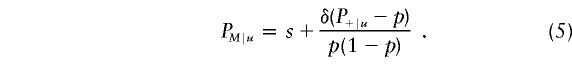Similar equations can be derived for the frequency with which an individual sampled from the lower end of the trait distribution will carry the M allele, P_M|l. Equations of this type have also been derived by Slatkin (1999) and Neilsen and colleagues (Nielsen et al. 1998; Nielsen and Weir ¹⁹⁹⁹), in slightly different contexts.

Testing LD: Power Considerations

The derivations above make it relatively easy to pursue power studies for test settings involving different marker and trait allele frequencies, interlocus distances, and LD strengths. Table 1 depicts a simple 2 × 2 contingency table that can be set up to assess the association between the marker-locus alleles and case-/control-subject status.

Table 1.

Basic Design for Investigating the Association Between a Marker Allele (or Haplotype) and Threshold-Defined Case and Control Subjects

Allele	Upper Percentile	Lower Percentile	Total
M	nupM|u	nlpM|l	n+
m	nu(pm|u=1-pM|u)	nl(pm|l=1-pM|l)	n-
Total	nu	nl=cnu	N

For present purposes, the statistic of interest that can be derived from the 2 × 2 table is the odds ratio

Schlesselman (1982) discusses calculations for assessing the power of tests of the hypothesis H₀:OR=1 (i.e., the marker locus is not in LD with the trait locus, or the locus being tested for LD does not have an effect on the trait of interest). In particular, if n_u is the number of case subjects in the study, n_l=cn_u is the number of control subjects (i.e., c is the control-subject:case-subject ratio and the total number of subjects is N=n_u+n_l), , , z_α is the quantile associated with a standard normal distribution for the (type I error) probability α, and

then, assuming relevant parameters have been set to hypothesized values, Ω={z_α,n_u,c,μ_--,μ_-+,μ₊₊,σ²,p,s,δ}, power can be calculated as

where φ(x|0,1) is the standard normal-density function evaluated at value x. Thus, given assumptions about a number of parameters—the trait-locus allele frequencies, locus-specific heritability and dominance effects, LD strength, marker-locus allele frequencies, thresholds for defining case-/control-subject status, number of case subjects, ratio of control to case subjects, and type I–error rate—one can compute the power to detect an LD-induced association between a biallelic marker locus and a QTL through tests of OR.

Results

In this section, we consider some computations involving the equations and derivations described in the previous section. We also showcase the effects of various parameters and assumptions on power to detect a locus effect. We perform the calculations in a few hypothetical situations, with the understanding that the reader may be interested in some unique or specific situations not overtly addressed in this paper. A computer program that can carry out the relevant calculations is available from the authors.

Conditional Marker Allele Probabilities

Table 2 offers some examples of calculations using equations 1–6 and ultimately gives the conditional probability that an individual sampled from the upper and lower ends of the trait distribution possesses an allele in LD with a trait-influencing allele. Note that when there is no dominance and the alleles are equally frequent (i.e., the value of p—that is, the column listed as p—is 0.5, and the value of d is 0), the quantiles used to define the upper and lower percentiles of the trait distribution are equal in absolute value, as expected.

Table 2.

Conditional Probability that an Individual Possesses a Trait-Value-Increasing Allele, Given that His or Her Trait Value Is in the Lower and Upper Percentiles of the Trait Distribution and under the Assumption of Different Trait-Locus Allele Effects^[Note]

		Locus Heritability		Probability (Threshold) for
Trait-LocusAlleleFrequency	d	Broad-Sense	Narrow-Sense	αl=.10	αu=.10	αl=.05	αu=.05	αl=.25	αu=.05
.5	.0	.333	.333	.155 (−1.580)	.846 (1.580)	.116 (−2.015)	.886 (2.015)	.234 (−.839)	.886 (2.015)
.5	.5	.360	.320	.088 (−1.420)	.759 (1.810)	.049 (−1.908)	.781 (2.212)	.197 (−.581)	.781 (2.212)
.3	.0	.296	.296	.060 (−1.917)	.660 (1.148)	.043 (−2.322)	.725 (1.598)	.098 (−1.222)	.725 (1.598)
.3	.5	.393	.367	.021 (−1.857)	.626 (1.481)	.012 (−2.284)	.654 (1.915)	.052 (−1.102)	.654 (1.915)
.1	.0	.152	.152	.013 (−2.174)	.312 (.601)	.010 (−2.551)	.375 (1.021)	.022 (−1.541)	.375 (1.021)
.1	.5	.265	.265	.004 (−2.164)	.391 (.826)	.002 (−2.543)	.454 (1.307)	.008 (−1.516)	.454 (1.307)
.5	1.0	.429	.286	.049 (−1.333)	.665 (2.111)	.021 (−1.865)	.667 (2.500)	.174 (−.360)	.667 (2.500)
.5	−1.0	.429	.286	.334 (−2.113)	.951 (1.330)	.334 (−2.502)	.981 (1.863)	.388 (−1.438)	.961 (1.863)
.3	1.0	.500	.412	.009 (−1.836)	.582 (1.863)	.003 (−2.273)	.586 (2.295)	.025 (−1.031)	.586 (2.295)
.3	−1.0	.247	.114	.231 (−2.228)	.667 (.668)	.231 (−2.599)	.811 (1.206)	.231 (−1.600)	.811 (.189)
.1	1.0	.381	.361	.001 (−2.160)	.454 (1.116)	.001 (−2.542)	.496 (1.681)	.002 (−1.505)	.496 (1.681)
.1	−1.0	.038	.007	.091 (−2.277)	.159 (.319)	.091 (−2.641)	.203 (.702)	.091 (−1.667)	.203 (.702)

Note.— For all runs, a=1. The table entries essentially give solutions to equation (3), with thresholds (in parentheses) defined as in equation (2); probabilities of possessing the allele are shown, given trait values in the lower α_l percentile and the upper α_u percentile.

Basic Sample-Size-Requirement Studies

Table 3 offers some examples of sample-size-requirement calculations for some select assumptions about the trait and marker-locus allele frequencies, dominance and locus effects, and LD strength. Table 3 makes it clear that if the trait-locus effect is modest (e.g., ∼20% of the variation explained) and/or the trait-locus allele frequency matches the associated marker-locus allele frequency, then it might be possible to detect an effect with realistic sample sizes even at genomewide rates. These are meant as examples only, since there are an infinite number of situations one might want to consider in terms of power. It is important, however, to consider the impact that assumptions about the potential locus effect—and, more importantly, the sampling scheme—have on power. We focus on the effects of some of these parameters in isolation in the sections that follow.

Table 3.

Sample Sizes Necessary to Detect an Association between a Marker Locus and a Trait-Influencing Locus Assuming Different Values for the Trait-Locus Allele Frequencies, Locus Effect Sizes, and LD Strength^[Note]

			Necessary Sample Size for Assumed Model ofInheritance and Assumed Type I–Error Rate
			Dominant		Recessive		Additive
Trait-LocusAlleleFrequency	LD (D′)	Locus-SpecificHeritability(LocusEffect)	.05	.00001	.05	.00001	.05	.00001
.10	.75	.10	150	425	1,001	2,856	140	394
.10	.50	.10	330	941	2,215	6,318	305	871
.10	.25	.10	1,297	3,700	8,701	24,819	1,197	3,415
.10	.75	.20	77	220	974	2,778	71	203
.10	.50	.20	172	482	2,154	6,143	156	444
.10	.25	.20	650	1,855	8,458	24,126	602	1,716
.25	.75	.10	56	160	105	302	48	135
.25	.50	.10	125	357	229	655	106	305
.25	.25	.10	500	1,427	885	2,524	417	1,191
.25	.75	.20	29	86	50	146	24	70
.25	.50	.20	67	193	110	315	113	157
.25	.25	.20	270	767	417	1,190	216	615

Note.— The associated marker-locus allele was assumed to have a frequency of .25, sampling was assumed to involve the upper and lower 10th percentiles of the trait distribution, and the power was assumed to be 80%. The entries reflect the number of case and control subjects (which are assumed to be sampled equally in number).

Influence of the definition of “extremes”

By sampling more and more extreme individuals, one can increase the power of an association study in certain instances. Figure 1 depicts power curves with the assumption that individuals have been sampled in a symmetrical way from the upper and lower percentiles of a trait distribution. Four different settings were studied with respect to sample size and locus effect (i.e., sample sizes of 100 and 50 case and control subjects, respectively, and locus-specific heritabilities of .1 and .25, respectively). It was assumed that the trait-locus effect was dominant, with the dominant allele having a frequency of .25 and an associated marker-locus allele frequency of .25. The marker and trait alleles were assumed to be in LD at 75% of the maximum for loci with the specified allele frequencies (assuming Lewontin’s D′ as scaled to a maximum achievable LD given allele frequencies [Lewontin ¹⁹⁸⁸]). A type I–error rate of .05 was also assumed. Figure 1 clearly shows that sampling more extreme individuals results in greater power. However, for the case subjects examined, the drop-off in power is not large if the sample is large or the locus effect is pronounced.

Figure 1.

Effect of sampling thresholds on the power to identify a QTL via association mapping. Simulating conditions were: D′ between trait/marker loci = 0.75, p_M = 0.25, and p₊ =.025, when the dominant model is assumed. Type I–error rate was set to .05.

Influence of the locus effect

Obviously, the larger the trait-influencing locus effect is, the easier it will be to detect an association between that locus and a marker-locus allele. Figure 2 depicts power curves for trait-locus–specific heritabilities ranging from .0 to .5 for samples of sizes 25, 50, 100, and 250 case and control subjects. The trait-locus allele was assumed to be dominant with a .25 frequency, and the associated marker-locus allele was assumed to have a frequency of .25. The marker and trait alleles were assumed to be in LD at 75% of the maximum for loci with the specified allele frequencies. Case and control subjects were assumed to be drawn from the upper and lower 25% of the trait distribution, respectively. A type I–error rate of .05 was also assumed. Figure 2 clearly shows that as the locus effect increases, the power increases greatly. Thus, even with relatively small sample size (∼50 case and control subjects), the power to detect a locus with a moderate effect, given the assumed sampling scheme, is quite good.

Figure 2.

Effect of the heritability of a QTL on the power to identify that locus via association mapping

Influence of LD strength

Clearly, if a marker locus and a trait-influencing locus do not have alleles in LD, then the marker-locus alleles will not act as good “surrogates” for the trait-influencing alleles. Thus, the strength of the LD between the marker and the trait-locus alleles is of extreme importance in detecting an association. It is important, therefore, to consider just how strong LD has to be before one can detect an association. Since the frequency of the alleles can have an impact on both LD strength and one’s ability to detect it, we have chosen to exemplify the influence of LD strength on mapping power by fixing the sampling strategy and locus effect parameters and varying LD strength and heritability. Figure 3 depicts the expected increase in power with increasing LD between the marker and trait loci. The trait-locus allele was assumed to be dominant with a .25 frequency, and the associated marker-locus allele was assumed to have a frequency of .25. Case and control subjects were assumed to be drawn from the upper and lower 25% of the trait distribution. A type I–error rate of .05 was assumed.

Figure 3.

Effect of LD strength between marker and trait loci on the power to identify a QTL via association mapping

Influence of Trait and Marker Loci Allele Frequencies

The single-locus test described here relies on the LD between the marker and trait loci, as shown in figure 3. Because LD strength is dependent on allele frequencies, it is also of interest to measure the simultaneous effects of marker and trait allele frequencies on power of the extreme sampling method. Figure 4 shows power as a function of SNP marker allele frequency for trait allele frequencies of .1, .2, .3, .4, and .5, when the disequilibrium between them is held constant at 75%, the maximum possible for the given frequencies. One hundred case subjects and 100 control subjects sampled from the upper and lower 10th percentiles of the trait distribution were assumed, as was a locus-specific heritability of 20%. The type I–error rate was set to .05. Although this plot demonstrates reasonable power for all of the trait allele frequencies, because of the high level of LD, it can be seen that the maximum power is achieved when the trait and marker allele frequencies are equal. This is intuitive and has implications for association studies, as described in the Discussion section. In addition, this issue has been addressed by others, in slightly different contexts (Schaid and Sommer 1994; McGinnis ¹⁹⁹⁸; Schaid and Rowland ¹⁹⁹⁸).

Figure 4.

Effect of quantitative trait and marker-locus allele frequencies on the power to identify the QTL via association mapping.

Influence of the definition of “control subject”

Often, in case/control studies, a researcher will sample individuals with a disease and then merely define control subjects as individuals without the disease. This definition of “control subject” can create a very heterogeneous group. As has been emphasized throughout this paper, for a quantitative phenotype, one can select control subjects who may lead to increases in mapping power, because they are less similar to the case subjects with respect to phenotype (i.e., their trait values are further removed from the case subjects’ trait values, making it less likely that they share genes for that trait). Figure 5 displays, in two ways, the effect of varying definitions of “control subject.” Figure 5A shows the increase in power with increasing number of control subjects, while keeping the other parameters constant. In this scheme, 100 case subjects were taken from the upper 25% of the trait distribution, and the varying number of control subjects was assumed to be sampled from the lower 25%. Under the conditions shown, reasonable power can be obtained from a control-subject/case-subject ratio <1, even for low heritability values. Figure 5B demonstrates the effect of varying the lower threshold of the trait distribution used for control subject sampling, while keeping the number of case subjects to control subjects constant at 100. One hundred case subjects were assumed to be sampled from the top 25% of trait distribution, the trait-locus allele frequency was assumed to be .25, the associated marker-locus allele frequency was also assumed to be .25, and the LD between the alleles was assumed to be 75% of its maximum and the trait-locus allele was assumed to be dominant. The type I–error rate was set to .05. Figure 5 shows that power decreases as less extreme control-subject–sampling thresholds are used. However, even for low heritability, the power for sampling control subjects from the lower half of the trait distribution is still quite good under the conditions studied.

Figure 5.

Effect of the definition of a “control subject” on the power to identify a QTL via association mapping. A, Power as a function of the number of control subjects sampled while keeping case-subject sample size and sampling percentiles constant (control subjects sampled from the bottom 25th percentile). B, Power as a function of control subject–sampling threshold while keeping case- and control-subject sampling sizes constant (100 each).

Discussion

Association mapping, although not without its problems, is enjoying a tremendous resurgence of interest because of the availability of polymorphic marker databases, high-throughput genotyping equipment, and a recognition of the limits of conventional linkage analysis mapping strategies for identifying the determinants of common complex diseases (Risch and Merikangas 1996; Collins et al. ^{1997, 1998}). A predominant issue that has arisen in the wake of this intense interest concerns the manner in which one should conduct an association study, especially with respect to quantitative traits. For example, many researchers have devised analogs of the standard transmission-disequilibrium test (TDT) for quantitative traits (see, e.g., Allison ¹⁹⁹⁷) with the hope that the advantages associated with the TDT (i.e., a control for population stratification) could be exploited (Spielman et al. 1993; Ewens and Spielman ¹⁹⁹⁵; Spielman and Ewens ¹⁹⁹⁶). Others have developed models for association analysis of quantitative traits that make use of fixed and random effects models for family-based collections (Boerwinkle et al. 1986; George and Elston ¹⁹⁸⁷; Amos et al. ¹⁹⁹⁶). These models have the clear advantage of allowing for the control or accommodation of residual genetic and familial effects on the trait. In addition, the sampling units—families or pedigrees—can be used in complementary linkage analysis studies as well (Schork 2000).

Unfortunately, the problem with both the TDT and random-effects–models approach is that they require family or (at least) parental information. Such information may be difficult or impossible to collect. Although one conceivably could collect a random sample of unrelated individuals and examine associations between a quantitative trait and marker-locus alleles, using analysis of variance and related statistical procedures, these strategies would not be optimal. The proposed sampling scheme, involving unrelated individuals sampled from thresholds defined by the trait distribution, is intuitive and can result in substantial power increases. In addition, many of the problems thought to plague case/control samples, such as stratification and cryptic heterogeneity, can be overcome with an appropriate use of DNA markers and analysis strategies (Pritchard et al. 2000; Schork et al., in press). Unfortunately, there are some drawbacks, both with the proposed method and with our derivations concerning its power. First, our derivations require knowledge of the trait distribution, so that relevant sampling thresholds can be defined. Rarely will one know the actual distribution of trait values in the population. However, large epidemiological studies often can estimate such distributions and therefore can provide approximate thresholds.

Second, our calculations assume that the trait values were distributed as normal variates, with constant variances across the genotype categories. It is unlikely that a trait will exhibit such homoscedasticity across genotype categories. It is also unlikely that a trait will exhibit perfect normality. This is especially true if multiple loci influence the trait of interest. Such multilocus influences can easily affect the power to detect a locus effect with simple sampling frameworks (Allison et al. 1998). We view our assumptions of normality and homoscedasticity as working assumptions. We encourage others to investigate alternatives.

Third, although we concentrated on single-locus associations, we recognize that haplotype and multilocus analyses might be more powerful. Haplotype and multilocus analyses may be able to exploit LD relationships among multiple markers and thereby make up for weak LD between any marker allele and the trait-influencing allele (Long et al. 1995; Clark et al. ¹⁹⁹⁸; Schork et al., in press). Unfortunately, power calculations assuming multiple haplotypes would be complicated to pursue. We therefore leave the details of such studies to further research.

One interesting facet of our study results concerns the effect of marker and trait-locus allele frequencies (e.g., table 3 and fig. 4). It is clear that, in certain situations, power increases in mapping will occur if the trait-influencing allele and associated marker-locus allele have the same frequency. This is likely due to the fact that if, for example, the associated marker-locus allele frequency is much greater than the trait-locus allele frequency, there will be many control subjects possessing the associated allele. This will obviously weaken evidence for an association, especially if the LD is weak between the trait and marker-locus alleles. The implications of this phenomenon for mapping studies are far-reaching. Consider the development and use of a map of markers that have similar allele frequencies. Such a map might not be ideal for detecting associations with alleles that have different allele frequencies from those of the markers. Overcoming this problem may be possible by studying haplotypic associations, which might provide greater specificity and matching of disease-allele frequencies. Obviously, greater research into this and related issues are needed.

Appendix: Notation

x	Trait value
−, +	Alleles at the trait-influencing locus
μg	Mean genotype effect:
σ2g	Variance of trait values associated with genotype g
σ2r	Variance of trait values, assuming equality of genotype variances
σ2G	Total trait variance caused by genetic effects at single locus
σ2a	Total trait variance caused by additive genetic effects at a single locus
σ2d	Total trait variance caused by dominance genetic effects at a single locus
p, q	Frequencies of the + and − alleles, respectively
fg	Frequency of trait-influencing genotype g
ρ(•)	Trait distribution in the population
a	+ allele effect
d	Dominance effect
HB	Broad-sense heritability
HN	Narrow-sense heritability
τu, τl	Threshold values for defining case and control subjects, respectively
αu, αl	Percentiles for sampling case and control subjects, respectively
M, m	Alleles at the marker locus
s, t	Frequencies of the M and m alleles, respectively
δ	LD strength between trait and marker alleles.
PM|u	Probability of possessing a marker allele given case-subject status
nu, nl	Number of case and control subjects, respectively
N	Total number of case and control subjects
c	Ratio of case subjects and control subjects
OR	Odds ratio for a 2 × 2 table assessing the marker and case/control status relationship
α, β	Type I– and type II–error rates
zα, zβ	α, β quantiles of the standard normal distribution.

References

- Allison D (1997) Transmission disequilibrium tests for quantitative traits. Am J Hum Genet 60:676–690 [PMC free article] [PubMed] [Google Scholar]
- Allison DB, Schork NJ, Wong SL, Elston RC (1998) Extreme selection strategies in gene mapping studies of oligogenic quantitative traits do not always increase power. Hum Hered 15:261–267 [DOI] [PubMed] [Google Scholar]
- Amos CI, Zhu DK, Boerwinkle E (1996) Assessing genetic linkage and association with robust components of variance approaches. Ann Hum Genet 60:143–160 [DOI] [PubMed] [Google Scholar]
- Boerwinkle E, Charkraborty R, Sing CF (1986) The use of measured genotype information in the analysis of quantitative phenotypes in man. I. Models and analytical methods. Ann Hum Genet 50:181–194 [DOI] [PubMed] [Google Scholar]
- Clark AG, Weiss KM, Nickerson DA, Taylor SL, Buchanan A, Stengard J, Salomaa V, Vartiainen E, Perola M, Boerwinkle E, Sing CF (1998) Haplotype structure and population-genetics inferences from nucleotide-sequence variation in human lipoprotein lipase. Am J Hum Genet 63:595–612 [DOI] [PMC free article] [PubMed] [Google Scholar]
- Collins FS, Guyer MS, Chakravarti A (1997) Variations on a theme: cataloging human DNA sequence variation. Science 278:1580–1581 [DOI] [PubMed] [Google Scholar]
- Collins FS, Patrinos A, Jordan E, Chakravarti A, Gesteland R, Walters L (1998) New goals for the U.S. Human Genome Projects: 1998–2003. Science 282:682–689 [DOI] [PubMed] [Google Scholar]
- Devlin B, Roeder K (1999) Genomic control for association studies. Am J Hum Genet Suppl 65:A83 [DOI] [PubMed] [Google Scholar]
- Ewens WJ, Spielman RS (1995) The transmission/disequilibrium test: history, subdivision, and admixture. Am J Hum Genet 57:455–464 [PMC free article] [PubMed] [Google Scholar]
- George VT, Elston RC (1987) Testing the association between polymorphic markers and quantitative traits in pedigrees. Genet Epidemiol 4:193–201 [DOI] [PubMed] [Google Scholar]
- Gu C, Todorov AA, Rao DC (1997) Genome screening using extremely discordant and extremely concordant sib pairs. Genet Epidemiol 14:791–796 [DOI] [PubMed] [Google Scholar]
- Jorde LB (1995) Linkage disequilibirum as a gene-mapping tool. Am J Hum Genet 56:11–14 [PMC free article] [PubMed] [Google Scholar]
- Lewontin RC (1988) On measures of gametic disequilibrium. Genetics 120:849–852 [DOI] [PMC free article] [PubMed] [Google Scholar]
- Long JC, Williams RC, Urbanek M (1995) An E-M algorithm and testing strategy for multiple locus haplotypes. Am J Hum Genet 56:799–810 [PMC free article] [PubMed] [Google Scholar]
- MacLean C, Morton N, Elston R, Yee S (1976) Skewness in commingled distributions. Biometrics 32:695–699 [PubMed] [Google Scholar]
- McGinnis RE (1998) Hidden linkage: a comparison of the affected sibpair (ASP) test and transmission/disequilibrium test (TDT). Ann Hum Genet 62:159–179 [DOI] [PubMed] [Google Scholar]
- Nielsen DM, Ehm MG, Weir BS (1998) Detecting marker-disease association by testing for Hardy-Weinberg disequilibrium at a marker locus. Am J Hum Genet 63:1531–1540 [DOI] [PMC free article] [PubMed] [Google Scholar]
- Nielsen DM, Weir BS (1999) A classical setting for associations between markers and loci affecting quantitative traits. Genet Res 74:271–277 [DOI] [PubMed] [Google Scholar]
- Pritchard JK, Rosenberg NA (1999) Use of unlinked genetic markers to detect population stratification in association studies. Am J Hum Genet 65:220–228 [DOI] [PMC free article] [PubMed] [Google Scholar]
- Pritchard JK, Stephens M, Rosenberg NA, Donnelly P (2000) Association mapping in structured populations. Am J Hum Genet 67:170–181 [DOI] [PMC free article] [PubMed] [Google Scholar]
- Risch N, Merikangas K (1996) The future of genetic studies of complex human diseases. Science 273:1516–1517 [DOI] [PubMed] [Google Scholar]
- Risch N, Zhang H (1995) Extreme discordant sib pairs for mapping quantitative trait loci in humans. Science 268:1584–1589 [DOI] [PubMed] [Google Scholar]
- Schaid DJ, Rowland C (1998) Use of parents, sibs, and unrelated controls for detection of associations between genetic markers and disease. Am J Hum Genet 63:1492–1506 [DOI] [PMC free article] [PubMed] [Google Scholar]
- Schaid DJ, Sommer SS (1994) Comparison of statistics for candidate gene association studies using cases and parents. Am J Hum Genet 55:402–408 [PMC free article] [PubMed] [Google Scholar]
- Schlesselman JJ (1982) Case-control studies. Oxford University Press, New York [Google Scholar]
- Schork NJ (2000) Genome partitioning and whole genome analysis. In: Rao DC, Province MA (eds) Advances in genetics. Academic Press, New York [DOI] [PubMed] [Google Scholar]
- Schork NJ, Allison DB, Thiel B (1996) Mixture distributions in human genetics research. Stat Methods Med Res 5:155–178 [DOI] [PubMed] [Google Scholar]
- Schork NJ, Fallin D, Thiel B, Xu X, Broeckel U, Jacob HJ, Cohen D (2000) The future of genetic case/control studies. In: Rao DC, Province MA (eds) Advances in human genetics. Academic Press, New York [DOI] [PubMed] [Google Scholar]
- Slatkin M (1999) Disequilibrium mapping of a quantitative trait locus in an expanding population. Am J Hum Genet 64:1764–1772 [DOI] [PMC free article] [PubMed] [Google Scholar]
- Spielman RC, McGinnis RE, Ewens WJ (1993) Transmission test for linkage disequilibrium: The insulin gene region and insulin depedent diabetes mellitus (IDDM). Am J Hum Genet 52:506–516 [PMC free article] [PubMed] [Google Scholar]
- Spielman RS, Ewens WJ (1996) The TDT and other family-based tests for linkage disequilibrium and association. Am J Hum Genet 59:983–989 [PMC free article] [PubMed] [Google Scholar]
- Xu X, Rogus JJ, Terwedow HA, Yang J, Wang Z, Chen C, Niu T, Wang B, Xu H, Weiss S, Schork NJ, Fang Z (1999) An extreme-sib-pair genome scan for genes regulating blood pressure. Am J Hum Genet 64:1694–701 [DOI] [PMC free article] [PubMed] [Google Scholar]