Deep mantle structure and the postperovskite phase transition

Abstract

Seismologists have known for many years that the lowermost mantle of the Earth is complex. Models based on observed seismic phases sampling this region include relatively sharp horizontal discontinuities with strong zones of anisotropy, nearly vertical contrasts in structure, and small pockets of ultralow velocity zones (ULVZs). This diversity of structures is beginning to be understood in terms of geodynamics and mineral physics, with dense partial melts causing the ULVZs and a postperovskite solid–solid phase transition producing regional layering, with the possibility of large-scale variations in chemistry. This strong heterogeneity has significant implications on heat transport out of core, the evolution of the magnetic field, and magnetic field polarity reversals.

The Earth's crustal structure is amazingly complex, consisting of thin oceanic layers of high-density basaltic rocks with island continents of thick, low-density sialic rocks. These islands move about, changing direction from time to time within the overall dynamic system, as defined by the plate-tectonics revolution of the 1960s. On a large scale, the relation between the locations of these continental blocks and deep mantle structure is beginning to be understood. Around the circum-Pacific, there is a well developed pattern of subduction that overlies most of the high-velocity regions in the lower mantle, which can be attributed to convective downwelling of cooled oceanic slabs. The high-velocity regions surround two regions of low velocities beneath the mid-Pacific and South Africa (Fig. 1), which we will designate as large low-velocity provinces (LLVPs). If large volcanic fields of lava or igneous provinces at the surface are restored to their eruption locations in a fixed frame of reference relative to plate motions, they concentrate above these two LLVPs (1). There also appears to be a correlation between the location of the LLVPs and anomalous velocity features present in the upper layers of the solid inner core (2). Thus, it appears that the heterogeneous structure of the lower mantle plays a role in the heat engine driving both the dynamo and plate tectonics; understanding images such as those displayed in Fig. 1 in terms of geodynamics and mineral physics becomes key (3).

Fig. 1.

Tomographic map displaying the D″ region of the lowermost mantle (300-km layer), the fast ring around the Pacific, and the two large, slow areas beneath the mid-Pacific and South Africa. The relatively fast patches, SGLE (30), SYLO (31), SYLI (52), and SLHA (17), indicate where shear-wave velocity jumps have been detected near the CMB. The shallowest velocity jump occurs beneath the fastest region (SGLE), which we suppose is the coldest region and becomes a candidate for the location of a mineral phase change (perovskite to PPV). Black dots give the locations where particularly strong ultralow velocity zones have been detected.

The image in Fig. 1 is similar to those produced by long-period tomographic techniques (for a review, see ref. 4). Refs. 5 and 6 argue that shear velocity (V_s) is reduced in the LLVPs but that compressional velocity (V_p) is only slightly reduced. This discordance in seismic velocities cannot be accounted for by purely thermal effects. Normal mode analyses suggest that these regions may have higher density (7) and may therefore be chemically distinct (8). The precise thermal and chemical combination that could account for the LLVPs is not yet resolved, but iron enrichment of relatively hot material is a likely scenario, leading to competition between thermal and chemical effects on the buoyancy of the LLVP material. In a dynamic mantle system, the LLVPs are good candidates as dense piles of chemically distinct material beneath midmantle upwellings (9). Resolving details of the seismic structure is essential for appraising this possibility.

Seismic resolution of the finer structure in the deep mantle can be obtained by using body-wave tomography, with structure in some regions being imaged for dimensions of a few hundred kilometers (10, 11). In one or two regions, high-velocity quasi-tabular structures can be traced from subduction zones to near the core–mantle boundary (CMB) (Fig. 1), compatible with whole-mantle convection models (12). Continuous structures are not found beneath all subduction zones, but lateral and radial gaps in down-wellings are expected as a result of time-varying plate tectonics (13). The sharpness of the features presented in Fig. 1 and their lateral transitions between regions of red (slow) and blue (fast) will be addressed in this review, where we argue for the presence of complexity comparable to that at the Earth's surface. Although we will discuss the global image, we concentrate on the end-member features in Fig. 1, which we will interpret as being associated with down-wellings (high velocity) and upwellings (low velocity) in the mantle.

Tomographic methods have proven successful in mapping out lateral variations in volumetric structure, but they intrinsically smooth out sharp jumps in seismic velocity. Waveform modeling can be useful for resolving strong velocity gradients, but there are many challenges in imaging complete 3D structures because of lack of waveform data coverage. The two methods complement each other, and comparing observed waveforms with synthetic seismograms generated for models based on tomographic images can be used as a starting point for sharpening features required to fit the waveform data, if necessary. One can view this process in terms of tomography providing the large-scale geographic framework for the detailed “geologic features” sensed by waveform modeling. We summarize some aspects of waveform modeling for complex lower mantle structures in “Appendix A” in Supporting Appendices, which is published as supporting information on the PNAS web site.

In this review, we first summarize some salient aspects of waveform modeling for complex lower mantle structure and then assess constraints on the LLVP beneath Africa and the high velocity under circum-Pacific regions. We then assess dynamical and mineral physics interpretations of deep mantle structures.

The African LLVP

The largest LLVP structure occurs beneath South Africa, as shown in Fig. 1. A 2D section through this massive anomaly is displayed in Fig. 2, where a tomographic image is compared with a sharp-walled structure. The latter was constructed by enhancing tomographic models and adding sharp boundaries guided by the waveform behavior. In its present form, it is halfway between a cartoon and a rigorously resolved structure. However, it quantitatively accounts for a large collection of record sections containing S, SKS, and ScS arrivals from suites of events and station combinations (14, 15). The structure appears to be isotropic, with nearly uniform 3% low shear velocity, no P velocity anomaly, and no clear horizontal discontinuity at the upper boundary of the structure, which extends well upward into the mantle, as shown in Fig. 2.

Fig. 2.

Shear velocity tomographic section (53) connecting South America to South Africa. The heavy green line indicates the sharp boundary where the shear velocities inside the structure are reduced by 3% relative to PREM. The principal ray paths, S and ScS (red) and SKS (green), sample the structure for epicentral distances 83–95°.

Perhaps the most convincing type of data demonstrating these sharp walls is presented in Fig. 3. In particular, seismic array recordings, including the SKS arrival, have paths that cross the southwestern boundary with a step-like change in travel time occurring near 100°. These data do not show significant multipathing; however, the 5-s change in arrival times is sizable. The difference in travel time across the boundary requires a structure extending 1,000 km upward from the CMB if the S velocity is reduced by 3%. Tomographic models predict less than half of this, with the velocity decrease smoothed over 5° (15). The map in the Fig. 3 Lower displays the spatial pattern of the travel time jumps (transition from blue to red symbols) for various observations of SKS and SKKS projected to the core exit points at the CMB. Data traversing the northeastern flank of the structure, where there is another velocity transition, do show multipathing, suggesting a sharp lateral gradient in structure (16).

Fig. 3.

Direct observational evidence for anomalous region beneath South Africa. Upper displays the South African array data from a shallow East Pacific rise event (970529) before and after shifting for alignment. The black arrow in Lower denotes the azimuth of ray paths from the event. Lower presents the SKS and SKKS travel time delays projected onto the CMB indicating the structural definition near the array; red triangles are 5 s late relative to PREM (blue). Note the jump in travel times near 101° when crossing the proposed large-scale African Low Velocity Structure (ALVS). The background color displays the geoid anomaly (in meters), which appears to be well correlated with the largest SKS delays, suggesting a dynamic relationship. Vectors indicating the preferred azimuth–distance orientation of the boundary relative to the array are discussed in the text.

Seismologists usually plot record sections of seismograms as functions of distance shifted in time to align according to a model, as displayed in Fig. 3. When searching for vertical structures, exploration seismologists sometimes plot data at constant distance but varying with azimuth (fan shots). Essentially, we can test directly for the presence of deep vertical structures by examining how wavefronts arrive at large arrays both with distance and with azimuth. The vectors in Fig. 3 indicate the directions of maximum horizontal gradient (see “Appendix B” in Supporting Appendices).

Circum-Pacific High-Velocity Provinces

Whereas the LLVPs appear to be dominated by extensive low-velocity volumes with strong lateral gradients in structure on their margins, the deep mantle regions underlying the circum-Pacific are consistent with more traditional horizontal layering. One of the initial indications that these regions are special was reported in ref. 17. This paper predates tomography and associated models with a lower mantle shear velocity discontinuity (Fig. 4). The basic discovery was that there is an extra seismic pulse arriving between S and ScS at ranges from 75° to 80° (Fig. 4). Seismogram sections as functions of distance display alignment of phases traveling along various paths in the mantle, and this extra arrival is readily apparent. The S wave travel time curve branches AB, BC, and CD comprise a triplication; corresponding multiple branches are commonly observed for paths in the crust and upper mantle due to horizontal velocity increases at depths near 410 and 660 km (18). The amplitude and timing of Scd (refracted by a high-velocity layer in the D″ region) relative to S (turning in the midmantle) show considerable regional variation (for a review, see ref. 19), but Scd is commonly observed in lower mantle regions with high shear velocity in tomography models. Simple (1D) layered structures have been proposed for the four regions highlighted in Fig. 1: SGLE (northern Siberia), SYLO (Alaska), SYL1 (India), and SLHA (Central America). Note that model SGLE has the most elevated boundary, which occurs in the fastest region sampled. Such models are not unique, and model SGHD120, which has a strong velocity gradient overlying a 1% discontinuity, fits the data (Fig. 4) as well as model SLHA, which has a 2.75% velocity jump. A 1% discontinuity without the added gradient produces a very weak Scd arrival over a narrow distance range (20). Synthetics generated for tomographic models such as those presented in Fig. 1 do not produce significant Scd arrivals unless the velocity gradients and contrasts are enhanced (21). The profile of seismograms labeled 2D in Fig. 4 is for a model obtained by applying a simple mapping operator to a 2D section of the tomographic model of ref. 11. This model matches the data as well or better than any 1D model, because it shares the common feature of having a laterally extensive high-velocity layer in D″. Overall, these regions are quite distinct from the LLVPs; the average D″ velocity is 1–3% faster than the Preliminary Reference Earth Model (PREM), strong gradients in velocity with depth are found from 200 to 300 km above the CMB, and lateral margins of the structure are not as clearly defined. While P wave velocity discontinuities have been reported, it appears that P wave structure is less pronounced than shear wave structure in most regions. The shear velocity discontinuity appears to be consistent with the onset of anisotropic structure, because the boundary appears sharper for horizontally polarized shear waves relative to vertically polarized shear waves.

Fig. 4.

Display of models and synthetic seismograms generated from such models. Upper Left displays the models derived from triplication data obtained from the four special regions introduced in Fig. 1. Also included are the standard earth model (PREM) and a hybrid model (SGHD120). Upper Right is a triplication curve for the S phase containing the secondary arrival (Scd), which arrives between S and ScS from 75° to 85°. Lower displays the comparison of TriNet array observations (California) with predictions from the hybrid model (SGHD120) and a 2D structure simulated from Grand's tomographic map. The traces are aligned on S travel times from PREM, eliminating station delays.

Dynamic Model Considerations

To gain insight into what type of fine-scale seismic attributes can be related to lower mantle scenarios involving chemical and phase-change boundaries, we conducted tests on dynamic models. Following such an approach, Sidorin and Gurnis (22) investigated the consistency between the standard PREM and adiabatic predictions for (MgFe)SiO₃ perovskite and (Mg,Fe)O magnesiowüstite models. They produced a model with a 50/50 mixture of these two minerals with a (Fe/Mg) ratio of ≈10%. This parameterization was then used to convert temperature difference, ΔT, from a standard temperature model (23) into a shear velocity anomaly for a whole-mantle convection model, as in Fig. 5. A purely thermal slab that reaches the CMB will have insufficiently sharp lateral shear velocity gradients to produce a triplication in S waves (20). Thus, an additional factor is needed to account for the shear velocity increases observed in D″ below circum-Pacific regions.

Fig. 5.

Generation of synthetic seismograms obtained from theoretical dynamic mapping. (Upper Left) Temperature profile for a dynamic model of a subducting slab and hot thermal boundary layer interacting with an exothermic phase transition. The thin solid line shows a phase transition with a Clapeyron slope of +6 MPa/K, a density jump of 2%, and an ambient height 180 km above CMB. (Lower Left) Shear wave velocities (shown in red) calculated for the three cross sections indicated. (Right) Synthetic seismograms calculated for the 2D velocity models (20). Note that profile A will produce synthetic seismograms containing a realistic Scd pulse between S and ScS comparable to those in Fig. 4.

The introduction of a chemical layer above the CMB increases the complexity of the convection problem but can be understood in terms of two Rayleigh numbers, one caused by the temperature differential (ΔT) and the other caused by the chemical density difference (Δρ). Their ratio

is called the buoyancy number, which also contains the coefficient of thermal expansion α. This number largely determines the stability and morphology of a dense layer embedded at the base of the mantle and is commonly used in both numerical and dynamical experiments (22, 24–26). A moderately thick chemical layer can remain distinct for 400 million years or more if it has a density difference of at least 2% and/or a particularly low α value. A thicker layer with a lesser density anomaly can persist for billions of years. Characteristics of such models are that the layer thickens beneath upwellings and thins toward down-wellings. Reconciling a chemically distinct layer with seismic observations presents a challenge; the clearest evidence for layering in D″ is beneath midmantle regions that are relatively high velocity. Down-welling in the midmantle, possibly involving slab material, should depress the boundary in these regions relative to surrounding areas. But shallower discontinuities are not observed in areas where midmantle down-wellings are not expected. Some areas, such as the central Pacific, appear to have a D″ discontinuity, but it is at about the same depth as in circum-Pacific regions (e.g., ref. 27). Thus, a compositionally distinct layer is hard to invoke unless midmantle flow is less pronounced than in whole-mantle convection scenarios and unless effects such as partial melting add to the compositional complexity (e.g., ref. 28).

An alternate possibility is that the velocity discontinuity in high-velocity regions is caused by a lower mantle phase change. A phase change model (Fig. 5) with a 2% shear velocity jump works well with the dynamical flow models, as shown by refs. 22 and 29. In this case, down-wellings can have both a thermal effect on the depth of the transition and an effect on the overlying velocity gradients, which influence the strength of the Scd arrival. Fig. 5 shows results for a phase change with a positive Clapeyron slope, which produces shallower transition in cooled mantle below down-wellings. The high-velocity regions near slabs produce strong Scd arrivals (profiles A and B), whereas the lower velocity upwelling region away from the subducted slab is predicted to have weak Scd arrivals (profile C). The temperature variations due to convection can combine with the Clapeyron slope of a phase transition to provide the flexibility needed to explain the observed regional variations in Scd strengths and timing differentials. In short, the dynamical studies favor a solid–solid phase change model with a modest (2%) velocity discontinuity, which can be augmented by velocity gradients in cold, high-velocity slab to produce a strong triplication. Global tomographic inversions do not incorporate the Scd phase, so that any travel time anomaly arising from a D″ discontinuity is attributed to volumetric structure in the deep mantle distributed over the depth range.

Further Consideration of a Deep Mantle Phase Change

Given the nonuniqueness of deep mantle seismic models, we reparameterized tomography models by adding a discontinuity at a certain level, h_pn, compensating for its influence on travel times by adjusting the local volumetric anomaly (Fig. 6). The velocity anomalies provided by the tomography model are mapped onto a fine mesh to ensure that the topography of the incorporated discontinuity is adequately resolved and that each vertical column of the new mesh is perturbed by adding a discontinuity with appropriate velocity compensation. To explore how well this composite model, with its incorporated first-order discontinuity, reproduces seismic observations, we computed 2D synthetic waveforms (21) for a variety of ray paths sampling D″ in four different regions (Fig. 1). The differential travel time T_Scd-S is obtained from the synthetic waveforms and compared with the corresponding observations for every event–station pair. These differentials provide important constraints on the D″ structure, characterizing the heterogeneity and possible topography of the discontinuity at the base of the mantle. We restricted the analysis of the quality of our model predictions to the T_Scd-S differential travel times used in determining the models in Fig. 6 and used the rms misfit to compare various models for a range of phase transition characteristics (γ_ph, h_pn), seeking compatibility with seismic observations. The two regions with the most consistent travel-time behavior involved regions beneath Asia (model SGLE) (30) and Alaska (model SYLO) (31). The differential times from these observations were used to test parameterized models,

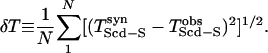The δT misfit errors are presented in Fig. 7 for a variety of h_pn, γ_ph models, where values in the neighborhood of h_pn = 200 km and γ_ph = +6 MPa/K fit the data the best.

Fig. 6.

A display of the steps taken in injecting a phase boundary into a tomographic model. (A) Shear velocity cross section along a great circle ray path from a South American earthquake (940808) to a typical North American station (SHW). (B) A perturbed vertical column incorporating an imposed discontinuity triggered by temperature and pressure. The dotted line shows PREM; the dashed line shows tomographic block anomalies. (C) Final composite model (perturbations with respect to PREM) for the region marked in A. The grid lines of the fine mesh are shown (every other line is plotted horizontally, and 1 in 10 is plotted vertically), and the phase boundary is indicated by the white line. The phase transition in B and C is characterized by h_ph = 200 km and γ_ph = 6 MPa/K.

Fig. 7.

Observed T_Scd-S differential travel time residuals from beneath Alaska and Eurasia, and predictions of models with various phase change characteristics. The shaded region marks the range of models providing the best fit to the data. Models within this region have approximately the same average elevation of the phase boundary above the CMB. They predict T_Scd-S with an average residual in the range of 1.8 to 3.4 s. The preferred model with the smallest residual is indicated by a plus sign (h_ph = 200 km, γ_ph =+6 MPa/K), although larger values of γ_ph are acceptable.

Until recently, there was not much support for a phase change in the lower mantle, but evidence suggesting a postperovskite (PPV) phase change has appeared, starting with experimental observations of a phase change in the end member, MgSiO₃, reported by Murakami et al. (32). This observation is supported by theoretical calculations indicating a sheet-like polymorph transition at D″ conditions, T = 2,750 K and P = 125 GPa, with bounds specified in Fig. 8. The new phase is predicted to be 1.5% denser than perovskite, and a positive Clapeyron slope of 7.5 MPa/K is computed theoretically. This estimate of the Clapeyron slope is slightly smaller than computed in ref. 33 (10 MPa/K), but similar estimates of T and P for the transition were given. Oganov and Ono (34) obtain values of 8 MPa/K with a velocity increase of ≈1.5% in shear velocity. At low temperatures, the PPV structure appears to be quite anisotropic, with V(SH) faster than V(SV) by ≈3% (32, 34), which is not found for the perovskite structure. This feature could explain shear wave splitting in D″ arrivals observed in refs. 35 and 36, but temperature effects reduce the difference in anisotropy between perovskite and PPV. Adding Fe complicates the behavior of the phase transition when including magnesiowüstite, as discussed in refs. 37 and 38, although, apparently, natural olivine containing both Mg and Fe does change into the new polymorph near D″ conditions.

Fig. 8.

Phase diagram of perovskite (open symbols) to PPV (filled symbols) assuming the end member Mg₂SiO₃. Squares and circles are from the results of refs. 32 and 34. The dotted lines indicate the expected T and P appropriate for the D″ region. The heavy, long-dashed line is the γ_ph = 6 predicted from last-century seismology, and the heavy black lines are from theoretical predictions (γ_ph = 7.5, straight lines) established in ref. 54. The short-dashed lines indicate the D″ zone of temperature and pressure.

Once we fix the reference model depth, h_ph, and adopt a γ_ph value along with a simple mapping of shear wave velocity into temperature, we can transform a tomographic image such as Fig. 1 directly into a map of PPV layer thickness, as presented in Fig. 9. This figure simply shows a thermal mapping, and any effects of chemical heterogeneity in the LLVPs are not accounted for. The relatively high γ_ph (6 MPa/K) predicts sharp gradients in the depth of the phase transition, as is apparent in many regions. In our predicted map, this gradient is particularly high beneath Central America, where the seismic data displays considerable variability, as noted in ref. 17. Some researchers (39) have divided the area into two patches separated near latitude line 15°N with separate 1D models SKNA1 (north) and SKNA2 (south). We used our model (Fig. 9) to predict the (T_Scd-S) differentials for their model, using the same event–station paths from their study. Our mapping procedure proves effective in explaining their (50 km) thickness change, as demonstrated in “Appendix C” in Supporting Appendices.

Fig. 9.

Map of the predicted elevation of the phase discontinuity (perovskite to PPV) assuming γ_ph =+6 MPa/K, with reference height of 200 km above the CMB, and tomographic model for the mapping (55). After ref. 29.

An even sharper gradient is reported in ref. 37 along the western edge of this structure, and in ref. 6, strong lateral variations in reflectivity of the discontinuity over small scale lengths beneath the Cocos plate are reported. Seismic wave migrations suggest that the D″ discontinuity decreases in depth by >100 km moving southward from Central America toward the equator (40), which is compatible with the predictions of Fig. 9. This region also has a complex subduction zone history, which could add to this complexity (13). In addition, a change in chemistry, perhaps aided by subducted material, could easily complicate the uptake of Fe in PPV as suggested in ref. 38.

The evidence for a D″ triplication beneath the Central Pacific is less convincing than for the zones indicated in Fig. 1, although some secondary arrivals between S and ScS can be identified by stacking (27). Fig. 9 predicts a deep discontinuity close to the CMB in this region because the low shear velocities suggest hot temperatures and a depressed phase boundary. According to our model, the primary reason for the weak Scd strength is the lack of fast material just above the D″ region; the model predicts weak arrivals, like for the CC′ plot in Fig. 5. Focused effort to detect such weak discontinuities is needed to test this idea, especially beneath the LLVP structures.

Perspective

It appears that the PPV phase is a good candidate to explain the seismic observations for the circum-Pacific patches indicated in Fig. 1, both in strength and depth of the Scd phase. One of the most attractive features of this interpretation of the seismic data is that it reconciles mantle dynamics, mineral physics, and seismology. Moreover, the ability to use an existing tomography model in conjunction with the reference PPV model (h_ph = 200, γ_ph = 6) to predict Scd results of observational samples not used in the inversion is, indeed, encouraging. However, even in these special regions where Scd is easily observed, there are reasons to be cautious. Tomographic models such as Grand's (11) have much less anomalous structure in the midmantle than is predicted by 2D dynamic models of subducted slabs. Part of the discrepancy could be caused by the usually complex, time-dependent plate histories (13). But as discussed earlier, the interplay between the volumetric anomalies in tomography structures and the PPV velocity jump has strong tradeoffs. That is, we could have enhanced the tomographic velocity anomalies, as for the African structure, and reduced the PPV velocity jump or the reverse. Thus, resolving continuous features of subducted material from the surface down to the deep mantle patches and the absolute strengths and dimensions of these features remains a fundamental issue. Moreover, because we can constrain subduction from paleo-plate reconstructions coupled with dynamic models, we have potential for a much better understanding of high-velocity regions. Similarly, the uplift rates (41) of South Africa can be used to constrain upwelling regions.

We did not include ScS timing in the above phase-boundary study or in the complete waveform modeling. The ScS timing depends strongly on the bottommost D″ structure. This zone may involve considerable complication due to the return of PPV to PV in the steep thermal boundary layer temperature gradient (42) and the interaction between a thermal-chemical layer with the PPV phase change (43). Some of such complexity is already embedded in the 2D studies like those in Fig. 6. Note the rapid changes in the phase boundary, even within the subducted material near position A. Recent detailed seismic modeling studies beneath the Caribbean support a great deal of complexity both in structure and anisotropic features on localized scales (3, 37). Addressing these issues requires more work on the mineral physics and better predictions of velocity properties as a function of temperature and chemistry.

If we accept the PPV hypothesis, we expect the lateral flow of cold slab material to concentrate anomalous dense materials at the CMB into piles (25, 44). These piles can form ridge-like appearances under certain circumstances (9) if slab history is imposed on a spherical Earth with a temperature-dependent rheology. The vertical extent of such piles depends on the density contrast, viscosity, thermal expansivity, etc. The high-density nature of the LLVPs appears to be supported by the mode analyses of ref. 7 and by modeling efforts invoking an iron-rich assemblage (8). The stability of such ridges remains in question for several reasons, including the uncertainty of the buoyancy number and the possibility of radiative transport of heat (45). The latter would allow hot-dense structure to remain much more isolated from convection, causing LLVPs to primarily affect the geometry of mantle circulation. If the African structure is controlled by convection, it must have distinct chemistry to sustain the sharp walls indicated in Fig. 3 (16). Furthermore, for the structure to be tilted away from the center of the anomaly, as in Fig. 2, requires that the thermal buoyancy be greater than the chemical buoyancy, which suggests that the LLVPs are unstable on geological time scales (46). Thus, the details of the structure become important for establishing its history and future predictions.

Probably the most anomalous structures at the CMB are the ultralow velocity zones (ULVZs) described in ref. 47. Although there is some debate about their lateral extent, most recent studies indicate that they are small, with lateral dimensions of 250–500 km and thicknesses of <50 km (dots in Fig. 1). Estimates of reductions of as much as 10% in P velocity and 30% in S velocity have been reported. Such small structures are difficult to study and can only be detected by subtle changes in waveforms (“Appendix D” in Supporting Appendices). Mineral physics has provided some evidence for dense partial melts in the lower mantle (48) that would probably sink to the CMB. Partial melts with modest melt fractions can have strong velocity effects, which may account for the ULVZs as discussed in ref. 49. The location of ULVZs near the edges of high-velocity regions has been addressed in ref. 13 and discussed in ref. 50. Why they occur along the edges of the African structure is less clear. Experiments with chemical heterogeneities suggest that partial melt could occur on the edges of chemically distinct piles (51). The seismic complexity of the deep mantle is beginning to fit into a framework of contributions from chemical heterogeneity, partial melting, and a phase transition, all embedded in a dynamic mantle flow regime (i.e., ref. 28). The recent discovery of the PPV phase has provided a major advance for interpreting seismological structures in the D″ region, and now a specific physical model can be tested against data. Extensive seismology, geodynamics, mineral physics, and geochemical modeling is still required to fully understand the lowermost mantle and its role in the mantle and geodynamo dynamic systems, but the recent rapid progress in these disciplines makes this task a viable undertaking.

References

- 1.Burke, K. & Torsvik, T. H. (2004) Earth Planet. Sci. Lett. 227, 531–538. [Google Scholar]
- 2.Niu, F. & Wen, L. (2001) Nature 410, 1081–1084. [DOI] [PubMed] [Google Scholar]
- 3.Lay, T., Garnero, E. & Williams, W. (2004) Phys. Earth Planet. Int. 146, 441–467. [Google Scholar]
- 4.Garnero, E. J. (2000) Annu. Rev. Earth Planet. Sci. 28, 509–537. [Google Scholar]
- 5.Masters, G., Laske, G., Bolton, H. & Dziewonski, A. (2000) in Earth's Deep Interior: Mineral Physics and Tomography from the Atomic to the Global Scale, eds. Karato, S., Forte, A. M., Liebermann, R. C., Masters, G. & Stixude, L. (Am. Geophys. Union, Washington, DC), Vol. 117, pp. 63–87. [Google Scholar]
- 6.Lay, T., Garnero, E. J. & Russell, S. A. (2004) Geophys. Res. Lett., 31, L15612. [Google Scholar]
- 7.Ishii, M. & Tromp, J. (1999) Science 285, 1231–1236. [DOI] [PubMed] [Google Scholar]
- 8.Trampert, J., Vacher, P. & Vlaar, N. (2001) Phys. Earth Planet. Int. 124, 255–267. [Google Scholar]
- 9.McNamara, A. K. & Zhong, S. (2004) J. Geophys. Res. 109, B07402. [Google Scholar]
- 10.van der Hilst, R. D., Widiyantoro, S. & Engdahl, E. R. (1997) Nature 386, 578–584. [Google Scholar]
- 11.Grand, S. P., van der Hilst, R. & Widiyantoro, S. (1997) GSA Today 7, 1–7.11541665 [Google Scholar]
- 12.Bunge, H. P., Richards, M. A., Lithgow-Bertelloni, C., Baumgardner, J. R., Grand, S. P. & Romanowicz, B. A. (1998) Science 280, 91–95. [DOI] [PubMed] [Google Scholar]
- 13.Tan, E., Gurnis, M. & Han, L. (2002) Geochem. Geophys. Geosyst. 3, 1067. [Google Scholar]
- 14.Ni, S. & Helmberger, D. V. (2001) Earth Planet. Sci. Lett. 187, 301–310. [Google Scholar]
- 15.Ni, S., Helmberger, D. V. & Tromp, J. (2005) Geophys. J. Int. 161, 283–294. [Google Scholar]
- 16.Ni, S., Tan, E., Gurnis, M. & Helmberger, D. V. (2002) Science 296, 1850–1852. [DOI] [PubMed] [Google Scholar]
- 17.Lay, T. & Helmberger, D. V. (1983) Geophys. Res. Lett. 10, 63–66. [Google Scholar]
- 18.Grand, S. P. & Helmberger, D. V. (1984) Geophys. J. R. Astron. Soc. 76, 399–438. [Google Scholar]
- 19.Wysession, M. E., Lay, T., Revenaugh, J., Williams, Q., Garnero, E. J., Jeanloz, R. & Kellogg, L. H. (1998) in The Core–Mantle Boundary Region, Geodynamics Series, eds. Gurnis, M., Wysession, M. E., Knittle, E. & Buffett, B. A. (Am. Geophys. Union, Washington, DC), Vol. 28, pp. 273–297. [Google Scholar]
- 20.Sidorin, I., Gurnis, M., Helmberger D. V. & Ding, X. (1998) Earth Planet. Sci. Lett. 163, 31–41. [Google Scholar]
- 21.Ni, S., Ding, X. & Helmberger, D. V. (2000) Geophys. J. Int. 140, 71–82. [Google Scholar]
- 22.Sidorin, I. & Gurnis, M. (1998) in The Core–Mantle Boundary Region, eds. Gurnis, M., Wysession, M. E., Knittle, E. & Buffett, B. A. (Am. Geophys. Union, Washington, DC), pp. 209–230.
- 23.Brown, J. M. & Shankland, T. J. (1981) Geophys. J. R. Astron. Soc. 66, 579–596. [Google Scholar]
- 24.Jellinek, A. M. & Manga, M. (2002) Nature 418, 760–763. [DOI] [PubMed] [Google Scholar]
- 25.Gurnis, M. (1986) J. Geophys. Res. 91, 11407–11419. [Google Scholar]
- 26.Davaille, A., Girard, F. & Le Bars, M. (2002) Earth Planet. Sci. Lett. 203, 621–634. [Google Scholar]
- 27.Russell, S. A., Reasoner, C., Lay, T. & Revenaugh, J. (2001) Geophys. Res. Lett. 28, 2281–2284. [Google Scholar]
- 28.Lay, T., Garnero, E. J., Young, C. J. & Gaherty, J. B. (1997) J. Geophys. Res. 102, 9887–9909. [Google Scholar]
- 29.Sidorin, I., Gurnis, M. & Helmberger, D. (1999) J. Geophys. Res. 104, 15005-l5023. [Google Scholar]
- 30.Gaherty, J. B. & Lay, T. (1992) J. Geophys. Res. 97, 417–435. [Google Scholar]
- 31.Young, C. J. & Lay, T. (1990) J. Geophys. Res. 95, 17385–17402. [Google Scholar]
- 32.Murakami, M., Hirose, K., Kawamura, K., Sata, N. & Ohishi, Y. (2004) Science 304, 855–858. [DOI] [PubMed] [Google Scholar]
- 33.Iitaka, T., Hirose, K., Kawamura, K. & Murakami, M. (2004) Nature 430, 442–445. [DOI] [PubMed] [Google Scholar]
- 34.Oganov, A. R. & Ono, S. (2004) Nature 430, 445–448. [DOI] [PubMed] [Google Scholar]
- 35.Matzel, E., Sen, M. K. & Grand, S. P. (1996) Geophys. Res. Lett. 23, 2417–2420. [Google Scholar]
- 36.Garnero, E. J., Maupin, V., Lay, T. & Fouch, M. J. (2004) Science 306, 259–261. [DOI] [PubMed] [Google Scholar]
- 37.Lin, J.-F., Struzhkin, V. V., Jacobsen, S. D., Hu, M. Y., Chow, P., Kung, J., Liu, H., Mao, H-k. & Hemley, R. J. (2005) Nature 436, 377–380. [DOI] [PubMed] [Google Scholar]
- 38.Mao, W. L., Shen, G., Prakapenka, V. B., Meng, Y., Campbell, A. J., Heinz, D. L., Shu, J., Hemley, R. J. & Mao, H-k. (2004) Proc. Natl. Acad. Sci. USA 101, 15867–15869. [DOI] [PMC free article] [PubMed] [Google Scholar]
- 39.Kendall, J.-M. & Nangini, C. (1996) Geophys. Res. Lett. 23, 399–402. [Google Scholar]
- 40.Thomas, C., Garnero, E. J. & Lay, T. (2004) J. Geophys. Res. 109, B08307. [Google Scholar]
- 41.Gurnis, M., Mitrovica, J. X., Ritsema, J. & van Heijst, J. (2000) Geochem. Geophys. Geosyst. 1, 1999GC000035. [Google Scholar]
- 42.Hernlund, J. W., Thomas, C. & Tackley, P. J. (2005) Nature 434, 882–885. [DOI] [PubMed] [Google Scholar]
- 43.Nakagawa, T. & Tackley, P. J. (2004) Geophys. Res. Lett. 31, L16611. [Google Scholar]
- 44.Tackley, P. J. (1998) in The Core–Mantle Boundary Region, Geodynamics Series, eds. Gurnis, M., Wysession, M. E., Knittle, E. & Buffett, B. A. (Am. Geophys. Union, Washington, DC), Vol. 28, pp. 231–253. [Google Scholar]
- 45.Badro, J., Rueff, J.-P., Vankó, G., Monaco, G., Fiquet, G. & Guyot, F. (2004) Science 305, 383–386. [DOI] [PubMed] [Google Scholar]
- 46.Conrad, C. P. & Gurnis, M. (2003) Geochem. Geophys. Geosyst. 4, 1031. [Google Scholar]
- 47.Garnero, E. J. & Helmberger, D. V. (1996) Geophys. Res. Lett. 23, 977–980. [Google Scholar]
- 48.Asimow, P. D., Sun, D., Akins, J. A., Luo, S. N. & Ahrens, T. J. (2005) Geochim. Cosmochim. Acta, in press.
- 49.Williams, Q., Revenaugh, J. & Garnero, E. J. (1998) Science 281, 546–549. [DOI] [PubMed] [Google Scholar]
- 50.Lay, T., Williams, Q. & Garnero, E. J. (1998) Nature 392, 461–468. [Google Scholar]
- 51.Gonnermann, H. M., Manga, M. & Jellinek, A. M. (2002) Geophys. Res. Lett. 29, 1029. [Google Scholar]
- 52.Young, C. J. & Lay, T. (1987) Phys. Earth Planet. Int. 49, 37–53. [Google Scholar]
- 53.Ritsema, J., van Heijst, H. J. & Woodhouse, J. H. (1999) Science 286, 1925–1928. [DOI] [PubMed] [Google Scholar]
- 54.Tsuchiya, T., Tsuchiya, J., Umemoto, K. & Wentzcovitch, R. M. (2004) Earth Planet. Sci. Lett. 224, 241–248. [Google Scholar]
- 55.Grand, S. P. (1994) J. Geophys. Res. 99, 11591–11622. [Google Scholar]
Associated Data
This section collects any data citations, data availability statements, or supplementary materials included in this article.