The Importance of Thermodynamic Equilibrium for High Throughput Gene Expression Arrays

Abstract

We present an analysis of physical chemical constraints on the accuracy of DNA micro-arrays under equilibrium and nonequilibrium conditions. At the beginning of the article we describe an algorithm for choosing a probe set with high specificity for targeted genes under equilibrium conditions. The algorithm as well as existing methods is used to select probes from the full Saccharomyces cerevisiae genome, and these probe sets, along with a randomly selected set, are used to simulate array experiments and identify sources of error. Inasmuch as specificity and sensitivity are maximum at thermodynamic equilibrium, we are particularly interested in the factors that affect the approach to equilibrium. These are analyzed later in the article, where we develop and apply a rapidly executable method to simulate the kinetics of hybridization on a solid phase support. Although the difference between solution phase and solid phase hybridization is of little consequence for specificity and sensitivity when equilibrium is achieved, the kinetics of hybridization has a pronounced effect on both. We first use the model to estimate the effects of diffusion, crosshybridization, relaxation time, and target concentration on the hybridization kinetics, and then investigate the effects of the most important kinetic parameters on specificity. We find even when using probe sets that have high specificity at equilibrium that substantial crosshybridization is present under nonequilibrium conditions. Although those complexes that differ from perfect complementarity by more than a single base do not contribute to sources of error at equilibrium, they slow the approach to equilibrium dramatically and confound interpretation of the data when they dissociate on a time scale comparable to the time of the experiment. For the best probe set, our simulation shows that steady-state behavior is obtained in a relaxation time of ∼12–15 h for experimental target concentrations ∼(10⁻¹³ − 10⁻¹⁴)M, but the time is greater for lower target concentrations in the range (10⁻¹⁵–10⁻¹⁶)M. The result points to an asymmetry in the accuracy with which up- and downregulated genes are identified.

INTRODUCTION

Single assay characterization of the response of thousands of genes to environmental perturbations is altering the research paradigm in biomolecular science. Applications are increasing explosively in areas as wide ranging as gene expression and regulation (Lashkari et al., 1997), genotyping and resequencing, and drug discovery and disease stratification (Eisen et al., 1998). The potential impact of micro-arrays on basic and applied biology is so important that an entire industry has been spawned, using any of dozens of variants of two generic methods to fabricate arrays—either direct deposition of probes (Schena et al., 1998; DeRisi et al., 1996; Duggan et al., 1999) or covalent attachment by in situ synthesis (Hughes et al., 2001; LeProust et al., 2000; Lipshutz et al., 1999; Singh-Gasson et al., 1999). The former method allows a wide range of substances such as presynthesized oligomers, proteins, cloned DNA, etc., to be used as probes. The latter is generally restricted to oligonucleotides but offers higher specificity.

The central theme of this article is the physical chemical limits of specificity; i.e., conditions that allow the best specificity we consider mainly, though not exclusively, arrays of 20–30 nucleotides long probes, manufactured by in situ synthesis. These conditions minimize false hybridizations resulting from the slow equilibration that is characteristic of long probes, and avoid competition between surface-bound and solubilized probes.

Typically an array of tens to hundreds of thousands of different pixels, each consisting of a homogeneous set of 1–10 million oligonucleotide probes, is used to determine the expression levels of genes of known sequence. The molecules to be assayed, e.g., cDNA, are hybridized, during a 12–15 h incubation, with probes chosen to be their reverse complements The most common detection method relies on fluorescence. Usually molecules from the target and reference cells are labeled with red and green dyes respectively; pixels are then scanned at the two distinct wavelengths to determine expression changes. Genes that are up- or downregulated in response to drugs, hormones, or other environmental influences are thus quickly identified.

Although micro-array assays are high throughput in the sense that in excess of 10,000 genes at a time are probed, the number of false-positives is high, even for arrays prepared by in situ synthesis. Increased specificity is typically achieved by sacrificing sensitivity: only genes with a pronounced change in expression level, typically in the fifth percentile, are scored as having changed. The screened set, or a select group of the screened set, is then investigated further using traditional methods such as Northern blotting.

Increased throughput is generally achieved by increased array density. However, as the above remarks imply, a substantial increase in throughput can be achieved by a well validated, high-specificity system. To increase specificity by rational design procedures, it is helpful to have a clear understanding of the physical limitations of the assay. This includes understanding the conditions that will provide the best specificity, the robustness to deviations from optimal conditions, the relation of optimal conditions to those prevalent in the most common experimental procedures, and strategies for optimization.

This article is divided into two broad components: equilibrium and kinetic. In the first section, we outline the thermodynamics of hybridization. Specificity and sensitivity are maximum when equilibrium has been achieved, but even under this ideal condition the method used to select probes affects the formation of crosshybrids, and thus it affects specificity. Probe selection is a large optimization problem. We discuss this below, and present a new probe selection method. Further below, we use this method to select probes for the full set of yeast genes and compare the specificities obtained at equilibrium where both specificity and sensitivity are maximum. This has particular implications for long probes inasmuch as length substantially reduces the rate at which equilibrium is approached, and consequently increases false-positives if equilibrium is not achieved.

Thermodynamics of hybridization

Melting profiles

As temperature is increased, an initially fully intact hybrid will gradually destabilize, and at high enough temperature, the strands will separate. Approximately 90% of the transition occurs over a temperature range of ∼10–15 degrees for 25-mers, with the range narrowing as length increases. The so-called melting curve, determined under equilibrium conditions, is cooperative and has an inflection point which is referred to as the melting temperature, T_m.

The melting temperature is defined as the temperature at which half the total number of strands are free (i.e., not hybridized). In general the population of hybridized strands will have a distribution of intact basepairs, and the arrangement of a given number of pairs will also be distributed. The common practice of neglecting partially hybridized states reduces a very complex multistage model to a two state model, eliminates the physical basis for cooperativity, and broadens the melting profile. For short chains, however, it has little affect on the midpoint of the transition, introducing an error that is within the error caused by experimental uncertainty in the stacking free energy.

For this two-state model in which partially hybridized states are neglected, a sequence-dependent expression for the melting temperature is easily obtained. Define β as the equilibrium constant for bimolecular nucleation (formation of the first bond) in units of inverse concentration, and let K be the (dimensionless) equilibrium constant for the formation of the remainder of the helix. For a helix with n bases, there will be n-1 stacking interactions. We write the sum of the standard Gibbs free energies for the n-1 stacks as ΔH−TΔS, so that the corresponding intramolecular equilibrium constant is , where ΔH and ΔS are the sums of the standard enthalpies and entropies for base stacking, in accordance with the base sequence.

The free energy of the nucleation event also, to some extent, depends on the basepairs that nucleate dimerization. If A be the free strand concentration and B the concentration of hybrids, and we assume the molecules are either fully hybridized or completely separated, then,

(1)

If c_T is the total strand concentration, then by conservation In addition, at the melting temperature T_m we have by definition 2B = A. Substituting these relations in the equation for B, and utilizing the definition of K, we have that,

(2)

The presence of a surface

The formation of a DNA hybrid consists of a bimolecular nucleation event followed by formation of a double helix. The main effect of the surface is to freeze the rigid body translational energy and entropy of half the free strands, and to restrict the approach between opposing strands to a half space. The result is to multiply all equilibrium constants by the same constant factor, which is entirely independent of oligonucleotide sequence. This will shift the temperatures at which helices destabilize by some sequence-independent factor. To first order, therefore, the presence of the surface does not affect conclusions about specificity. As we will show via simulation, the effect of the surface on kinetics is crucial, and has a pronounced influence on specificity if equilibrium is not reached.

Probe selection

To be specific, we consider arrayed probes to be 25 nucleotides (nt) long that hybridize to complementary targets from genes in the cells of interest. We will consider one target region per gene, although that restriction is easily relaxed.

For a gene N long and a target L long, there are N − L + 1 potential targets, each potential target being the exact reverse complement of a probe that recognizes it. To understand how choice of target affects accuracy, consider the extreme case in which targets are selected at random. Hybrids would then cover a wide range of melting temperatures. The experimental temperature (at which hybridization is carried out) must be chosen low enough to assure stability of all hybrids. But with that requirement met, the wide range of melting temperatures would result in many hybrids having melting temperatures well above the experimental temperature, and more importantly sequences that are similar to the targets (differing by one base, say), would also be stable at the experimental temperature, as would complexes between target regions and certain incorrect probes. The problem is exacerbated when the expression levels of the spurious targets are higher than the correct targets, and made even worse when equilibrium is not achieved.

At the chosen experimental temperature, therefore, we not only want to choose the target regions so that the reverse complements (i.e., the probes) have a small enough binding free energy to assure stable hybridization, but we also want the free energy of potentially incorrect hybrids to be high enough to assure that they do not form at the experimentally chosen temperature. It is evident from the previous paragraph that we can screen out large numbers of false hybrids and choose targets by minimizing the dispersion in correct probe–target melting temperatures, subject to the constraint that the free energies of correct hybrids render them stable at the experimental temperature, whereas the free energy of incorrect hybrids renders them unstable. The two constraints place upper and lower bounds on the free energies (Li and Stormo, 2001)

Screening the pool of potential probes

A genome with M bases and N genes will provide a pool of M − N(L − 1)segments of length L, from which N probes are to be selected, one per gene. For the yeast genome we use a number of screening procedures to focus on high-quality probe sets. Initial pruning is achieved by a suitable choice of melting temperature.

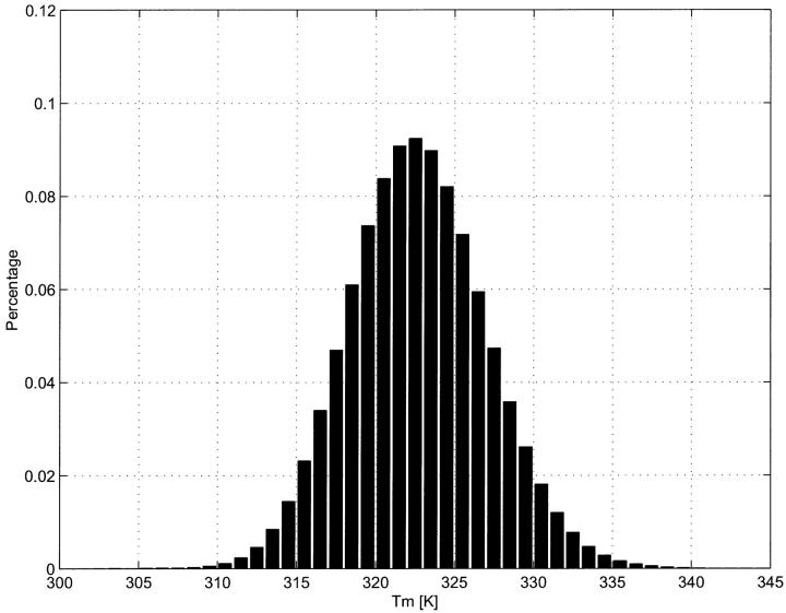
It is important to take care in setting the hybridization temperature. Choosing an experimental temperature low enough to assure stability of correct hybrids is important for good sensitivity, whereas choosing a temperature high enough to eliminate spurious hybrids is required for specificity. To find a suitable experimental temperature, we first obtain the distribution of melting temperatures of the entire potential pool of M − N(L − 1) correct hybrids (Fig. 1). For the yeast system (http://genome-www.stanford.edu/Saccharomyces), N = 6280 and M = 12,057,500, so that the required calculations can be easily done on a PC.

FIGURE 1.

Distribution of T_m of 25-nt DNA duplexes, pooled from the entire yeast gene set. At 0.3 M salt concentration, T_mm is ∼323 K. We choose probes whose T_m is in the range [319 K–327 K]. Experimental temperature is set to 315 K, so as to guarantee the sensitivity of the probes with the lowest T_m.

Calling the mean of this distribution T_mm, we restrict probes to a relatively narrow band of melting temperatures; specifically, we take only those probes having This constraint has two effects. First, it speeds probe selection by reducing the search space. Second, it guides the selection of the experimental temperature, which we take to be a few degrees below the lowest acceptable value of T_m.

Using this restricted pool of probes, and with melting temperature set, we generate probe sets to simulate hybridization experiments, to compare specificities, and especially to understand the implications of failing to achieve equilibrium.

Probe sets

We used both randomly generated and optimized probe sets. The algorithm to generate an optimized probe set (OPS) is divided into two stages. In the first stage, probes are screened on the basis of binding free energies and other properties that depend only on their sequence, and not the global characteristics of the set. This stage is similar to existing methods. In the second stage, the remaining probe candidates are screened further, using a target function designed to minimize cross-reactivity and maximize specificity between the probe and its complement.

Typical Stage I strategies to reduce crosshybridization are based on tuple frequency (personal communication, Olympus, http://www.olympus.co.jp) and the BLAST sequence search algorithm (C. Sugnet, E. Rice, and T. Clark, 1999, personal communication, http://arrayit.com/Services/ArrayDesign/arraydesign. html, http://www.basic.nwu.edu/biotools/Primer3.html). We use these strategies to make a first cut at the number of probe candidates. Specifically, in our Stage I screening, we eliminate sequences based on the following considerations.

Self-complementarity

It is particularly important to eliminate self-complementarity when insufficient time is allowed to reach equilibrium (as is almost always the case). At equilibrium, and depending on concentration, the ratio of bimolecular to intramolecular complexes might be high, but intermolecular reactions will always slow the kinetics of binding, thereby affecting sensitivity and possibly specificity.

Base composition

We exclude probes that are particularly AT- or GC-rich, in accordance with empirically based guidelines developed by Affymetrix (Lockhart et al., 1996).

Stability

Probes are selected so that the hybridization free energy is lower than some threshold. If experiments achieve thermodynamic equilibrium, this threshold determines the sensitivity to expression level. If G^* is the maximum allowed standard free energy of the duplex, relative to the singly nucleated dimer, the lowest detectable expression level will vary as e^−G*/RT, where T is the temperature at which hybridization is performed.

3′ bias

Dye is generally incorporated during reverse transcription when cDNA is synthesized. Reverse transcription rarely results in complete transcripts of the message; i.e., a substantial amount of 3′ bias is typical. For sequences N long, we eliminate from consideration as probe candidates, the N/3 bases closest to the 5′ end of the chain. In the second stage, we select probes to minimize crosshybridization. False-positives due to crosshybridization are often minimized empirically by adding pixels with probes that differ in a single basepair from the perfect complement. Although this procedure is helpful, there are problems with it of both a fundamental and pragmatic nature. The latter include cost and (for cells from most human tissue) insufficient quantities of pure mRNA.

The most direct way to choose the best probe set is to compute every crosshybrid free energy, and pick the probes that crosshybridize the least. It is, however, unnecessary to follow such a costly procedure. In particular we need only evaluate free energies of crosshybrids whose stability exceeds some reasonable threshold.

We generate a list of binding energies for all target–probe hybrids that have not been eliminated by restricting the melting-temperature range.

We let be the free energy of probe i for target k, with ΔG_kk the binding energy of the correct target to the probe k. We discriminate against probes that are more likely to crosshybridize by using the reciprocal of the correct binding fraction at equilibrium, with all genes referred to a common expression level. Thus, we define the quantity C(k) as,

(3)

It is clear that C(k) is always positive. The larger the value of C, the greater the crosshybridization. For each gene, we choose the probe with lowest C value among all possible probe candidates. If multiple probes are needed, we avoid using overlapping probes because they would compete for the same target and decrease the overall identification efficiency. The main problem with carrying out this procedure is that the search space grows as a power of the number of genes, , before melting-temperature pruning. This makes exhaustive computation of crosshybrid free energies prohibitive.

We have mitigated this problem by the algorithm outlined below, which uses a combination of lookup tables, and a very fast dead-end elimination procedure to obtain free energies. Our binding strand search consists of a fast heuristic step that narrows the search space, followed by a slower evaluation (dynamic programming) on high-ranking candidates. We break the query sequence into overlapping k-mers, where k is the minimum number of basepairs necessary to form stable duplexes (typically 6–12). Candidates are quickly located through k-mer indexes of the entire gene set and a synonym table, both of which have to be prepared once before any search is performed. An extension step is then performed to get the entire duplex.

Step 1: Index the entire gene set; create a list of the occurrence sites for each of the 4^k unique k-mers. Step 2: For each of the 4^k unique k-mers, find a list of k-mers, called synonyms, that have no more than M mismatches with the given k-mer. We calculate the synonym score, i.e., the base-stacking free energy for the k-duplex. We compute the base stacking energy with a nearest-neighbors model (Fotin and Mirzabekov, 1998), using SantaLucia's parameters (SantaLucia, 1998; Seneviratne et al., 1999). We only need to do this once for a given k. Step 3: Decompose the query sequence into overlapping k-mers. A query sequence of length L has L − K + 1 overlapping k-mers. Find all synonyms for each k-mer in the synonym table prepared in Step 2. For each synonym, every entry in the index table represents a potential site that binds the query sequence with high affinity. Step 4: Use dynamic programming to extended a potential binding strand at both ends, coupled with calculation of binding free energy, following Eq. (3).

We allow mismatches during this step, but stop when long mismatched segments (e.g., three mismatches out of four consecutive basepairs) are encountered, due to unavailability of parameters to predict free energies of such long loops and bulges. The hits are restored in a hash table, using the site of the hit as the key. Whenever two alignments are obtained for the same site, we keep the one with more favorable binding free energy.

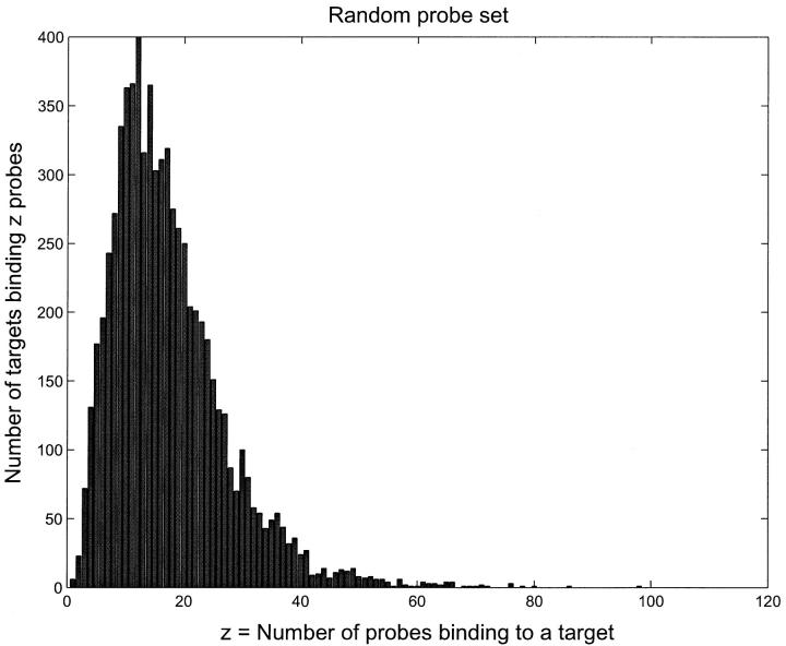
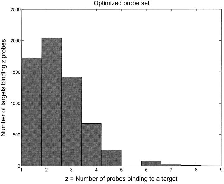
Our heuristic search algorithm focuses on short matched segments, which actually forms the “core” of the final duplex, inasmuch as the binding energy is more sensitive to the number of contiguous matching pairs than to the total number of matching pairs. This seamlessly combines a BLAST-like DNA sequence search with a calculation of binding free energies in such a way that the scores are no longer sequence similarities and E-values, but the ΔG values that are used to model the hybridization process. The specificity of the OPS compared to the random probe set (RPS) is evident from Figs. 2 and 3, where we show a histogram of the number of probes binding to a given target.

FIGURE 2.

Histogram of number of probes binding to a target with dissociation time greater than 1 s for the RPS. The median number of probes per target is sixteen. This should be compared to the OPS data in Fig. 2, where the median is between two and three.

FIGURE 3.

Histogram of number of probes binding to a target with dissociation time greater than 1 s for the OPS. The median number of probes per target is between two and three. In addition, the binding energy gap between the probe that binds best and the probe that binds next best is very large in all cases.

Notice that for the RPS, there are many probes that can bind to a given target. As we will see later, this leads to crosshybridization levels that are very high, making it virtually impossible to determine target concentrations from the probe binding amounts. On the other hand, for the OPS, only a few probes bind appreciably to any target. This almost eliminates crosshybridization and makes it possible to infer target concentrations quite well.

Kinetic simulations

Our in silico gene array consists of a two-dimensional square of size ∼2 cm × 2 cm which is divided into 80 × 80 pixels making up the x-y plane of the experiment. Each pixel has 10⁷ probes tethered to it, which are assumed to be identical and equivalent with respect to their binding properties to presented targets.

For concreteness, we will assume a liquid film of thickness 1/4 mm divided into five equal layers. The bottom layer is where the hybridization between targets and probes takes place. In the remaining layers above the bottom layer, the targets merely diffuse. Thus, our modeling space is made up of a regular grid of boxes of size δ_x,y, δ_x,y, δ_z in the x, y, z directions where δ_xy = 2 cm/80 = 0.025 cm and δ_z = 0.025 cm/5 = 0.005 cm.

We first experimented on the RPS to set limits on experimental parameters. The probes were placed on the two-dimensional grid at random locations. This is just a convenient placement of probes—and not necessarily optimal. The experiment consists of following the targets in time, allowing them to diffuse and hybridize. We track the number of targets of each type that are bound to each probe as a function of time.

To avoid issues with target–target interactions, we chose to model a middle range of target concentration of (10⁻¹⁵ − 10⁻¹³)M. The most favorable target–target binding energy is −35 kJ, whereas the most favorable binding energy between a probe and its appropriate target is −85 kJ. Hence, the ratio of affinities at T = 315K between probe–target and target–target interactions is greater than 2 × 10⁸. Moreover, the target concentration in our modeling is less than or equal to the probe concentration. From this one can conclude that the total target–target binding rate is negligible compared to the probe–target binding rate and we can neglect target–target binding.

We can then consider each target as if it were diffusing on its own. If N_T(x, y, z, t) is the number of target molecules of a specific type in a unit box centered at (x, y, z) at time t, then, the continuum diffusion equation for N_T can be written as:

(4)

Inasmuch as our targets are of size less than 100 nt we use a diffusion coefficient D = 10⁻⁶cm²/s (Chan et al., 1995). As we will show from our simulation, the precise value of D is not important. We rewrite the continuum diffusion equation as a difference equation. After some simple rearrangements, one gets:

(5)

Let us define the dimensionless probabilities D_xy in the x-y plane and D_z in the z direction as:

(6)

The diffusion equation can be interpreted as a molecular dynamics evolution for which we define an updating procedure at each time step as follows: for each box centered at (x, y, z), the average number of target molecules that are entering the box from the +x direction is and the number that are leaving the box to enter the box in the +x direction is We generate Poisson variables A⁺ and A⁻ with mean and bounded from above by N_T(x + δ_xy, y, z, t) and N_T(x, y, z, t) respectively (inasmuch as we cannot have more particles diffuse out than are present in the box). Thus the net flow into the box at (x, y, z) from the +x direction is Δ = A⁺ − A⁻. The quantity Δ is calculated for each direction for each box and the value of N_T is updated using these when they have all been calculated. For the z direction, the dimensionless coefficient D_z is used in place of D_xy.

This procedure works if the dimensionless constants D_xy and D_z are small enough so that they can be legitimately interpreted as probabilities. In our modeling, we chose D_z to be 0.2. This determines δt = 5s as our time step and D_xy = 0.008. Note that the probability to diffuse in the x-y plane is smaller by a factor of 25 compared to the probability to diffuse in the z direction. Thus, we are led to the approximation that once a target has diffused out of the bottom layer in the z direction, we may assume that it mixes perfectly with the layers above. This allows us to simulate a single layer in the z direction. After each time step, we recalculate the number of targets in the layers above the bottom layer and assume that they are distributed evenly in the layers above.

The diffusion step is followed by a binding step. Once again, this happens only in the bottom layer. The equation governing the binding step will now be considered. If [TP] is the number of target–probe complexes per mol, [T] is the number of free targets per mol and [P] is the number of free probes per mol, then,

(7)

It is easy to show that this equation can be transformed into an equation for the particle number. Thus if N_T, N_P, and N_TP are the number of particles of target, probe and target–probe pairs in the interaction region, then,

(8)

(9)

where, N_A = Avogadro's number, V = volume of liquid in which targets are placed = 10⁻⁴ liters, R_r = r_r, and I and J label the targets and probes, respectively.

The binding and unbinding process is now modeled by interpreting the above equations as follows. Each xy pixel corresponds to a single probe. For each probe, the average number of new target–probe pairs formed in a time step δt is where N_T(I) is the number of available targets of type I in the box and N_P(J) is the number of unbound probes in the box. We assume that there are no steric effects and all unbound probes have an equal chance to bind to the available probes. The actual new target–probe pairs formed in time δt is computed by generating a Poisson variable with mean δN_T(I)P(J). Similarly, one can compute the number of target–probe pairs unbinding by generating a Poisson variable with mean R_rN_T(I)P(J)δt.

Repeating this step over all the targets for all the boxes in the bottom layer of the array completes the binding–unbinding. A probe length of 25 nt gives an average melting temperature of 334 K at 0.3 M salt. The experimental temperature for our simulation, following the empirical rules described previously, is therefore set to 315 K.

Effect of diffusion

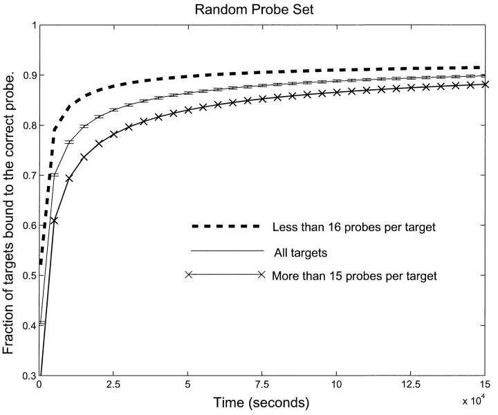
We first modeled the kinetics of hybridization for t varying from 0 to 150,000 s for the RPS. Fig. 4 shows the fraction of targets correctly bound (bound to the probe for which they have the lowest binding energy) as a function of time. We have separated the targets into two sets—those that bind to more than 15 probes and those that bind to less than 16 probes. These numbers were chosen to divide the target set into two sets which bind an equal number of probes in total. It is evident from Fig. 4 that even at t = 150,000 s, a significant fraction of the targets are bound to the wrong probes. This error is exacerbated in the targets that bind individually to a larger number of probes. In a normal gene array experiment, the hybridization is allowed to proceed for ∼12–15 h (40,000–50,000 s). Thus, for the RPS, our experiment shows that the “usual” procedure would yield a significant error.

FIGURE 4.

Fraction of correctly bound probes as a function of time for the RPS. Targets are separated by how many probes bind to them. The upper and lower curve correspond to targets with less than sixteen and more than fifteen probes respectively. The middle curve is the average over all targets. Notice that it takes longer than half a day to reach equilibrium and that, even at equilibrium, there is a significant fraction of targets that are incorrectly bound. Also note that targets which bind to more probes converge slower to a lower correctly equilibrated fraction. This means that, with this probe set, any experiment run for a finite time will have a systematic bias toward underestimating downregulated genes and overestimating upregulated genes.

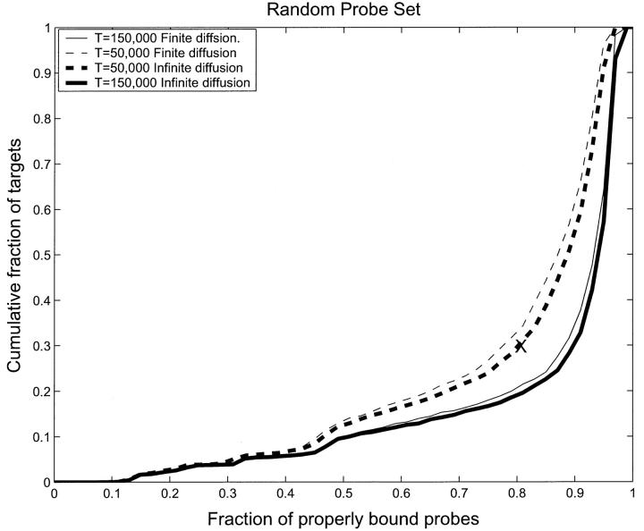
It is important to determine where the error in hybridization is coming from. One possibility is that it is due to the finiteness of the diffusion rate. To see if this is the case, we made the diffusion coefficient “infinite” by immediately redistributing all the unbounded target molecules of each type evenly among all the boxes after each binding step. Fig. 5 shows the comparison between finite diffusion and “infinite” diffusion for two time instances, t = 50,000 s and t = 150,000 s. It is evident from Fig. 5 that there is no significant difference between infinite diffusion and finite diffusion. However, it is clear that diffusion is important. Indeed, if we turn off diffusion completely, then the only binding will be for the small number of targets that are initialized in each box which can hybridize to the probes in that box. Fig. 5 shows that although diffusion is important, it is not the cause of the hybridization errors of Fig. 4.

FIGURE 5.

Cumulative fraction of properly bound targets as a function of the probability that a probe is properly bound for the RPS. Thus the point (0.8, 0.3) (marked with an X), represents the case when 30% of targets are correctly bound to their appropriate probe in less than 80% of the possible cases. Ideally, if everything was correctly bound, the curve would be zero for all values, except at unity when it would be unity. The trend toward this can be seen in the data. The dashed curves represent T = 50,000 s and the full curves represent T = 150,000 s. One observes a slow improvement in binding after T = 50,000 s, but perfect binding is never achieved, even in equilibrium. The thick lines, dashed and full, represent infinite diffusion as defined in the text, whereas the thin lines represent finite diffusion. The difference between these two is small.

Inasmuch as infinite and finite diffusion give almost the same result, and the infinite diffusion case is much faster to model, we will henceforth use the infinite diffusion limit. Note that this means that our modeling sets a lower bound on problems such as crosshybridization and target concentration measurements. Any real experiment, with a finite diffusion coefficient, can expect to see more severe effects than we see in our idealized experiment.

Effect of target concentration

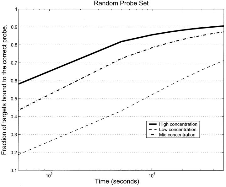
Another parameter that might affect the hybridization rate is the concentration of targets. We raised/lowered the target concentration by a factor of 10 and reran the simulation. The comparison of these with the original middle range concentration is shown in Fig. 6. It is clear from this that target concentration does play an important role in hybridization error. The higher the target concentration, the better the hybridization.

FIGURE 6.

Fraction of correctly bound targets for the RPS as a function of time for three different target concentrations, low, mid, and high, which correspond to 1.6 × 10⁻¹⁵M, 1.6 × 10⁻¹⁴ M, 1.6 × 10⁻¹³ M respectively. In none of the cases is equilibrium reached in the 12 h of hybridization. The equilibration rate depends strongly on concentration. This means that genes that are downregulated need longer times to be measured with the same accuracy compared to those that are upregulated. A simultaneous measurement of up- and downregulation will have a systematic bias toward upregulated genes.

Fig. 6 suggests that in a real gene array experiment, run for a finite time, at least for the RPS, concentrations of downregulated genes would be underestimated, whereas those of upregulated genes would be overestimated.

The role of probe specificity

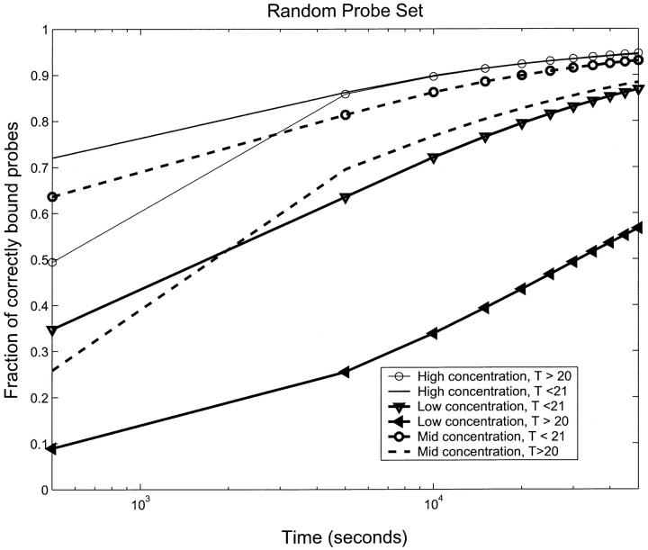
Crosshybridization is a serious problem in determining the expression levels (concentrations) of targets from the hybridization levels. Intuitively, it is clear that one will get more crosshybridization if a given probe binds to many targets. Fig. 7 shows the average fraction of properly bound probes (those bound to the targets that bind to them with lowest binding energy) for different target concentrations for the RPS as a function of target concentration. We have separated the probes into two sets of approximately the same size—those that bind to fewer than 21 targets and those that bind to more than 20. Fig. 7 shows clearly that at all target concentrations, the probes that have the largest number of targets binding to them show the biggest errors in hybridization. For the high concentration experiment, the fraction of correctly bound probes for the two sets merged into a single curve after ∼50,000 s. However, at the other two concentrations, the two sets do not come together even after 150,000 s (42 h). This indicates the need to optimize probe–target specificity, as was done in selecting the OPS. We would expect, and we will show that this is indeed true, that these types of errors will be much reduced with the OPS.

FIGURE 7.

The fraction of correctly bound probes as a function of time for the three concentrations, high, mid, and low with the RPS separated into two subsets—those that bind less than 21 targets and those that bind more than 20 targets. The worst case is low concentration, where the total fraction correctly bound is small. There is also a very significant dependence on how many targets bind to the probes. For the high concentration case, the dependence on number of binding targets is not important after T = 40,000 s. We see that an important source of error in identifying targets from bound probes is the concentration. Even after long times, a low enough concentration will have a significant error. A second source of error is crosshybridization error from large numbers of targets binding to a given probe.

Simulations on the optimized probe set

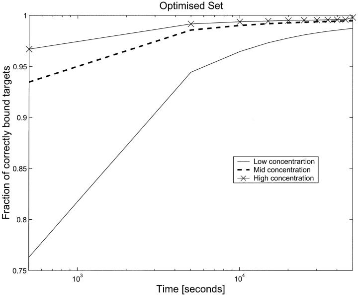
Fig. 8 shows the results of simulations on the OPS for low, high, and midtarget concentrations. At T = 40,000 s, the high concentration targets have an average error of less than one-half percent. If one looks at the probe set carefully and computes the targets that will bind best to each probe, one finds that there is a unique probe–target match, except for a single probe. In addition, if one uses the binding energies to compute the asymptotic fraction of incorrectly bound targets for each probe, one finds that this is less than 1% in all cases (except for two probes for whom the fraction is between 5 and 7%). This means that for the optimized probe set, the issue of asymptotic incorrect binding which plagued the RPS is resolved. The only issue that remains is that the time needed to reach equilibrium depends on target concentration. For the cases we modeled, the low concentration simulation had not reached a state of asymptote even after 50,000 s. However, unlike the situation for the RPS, where waiting longer would result in a large fraction of incorrectly bound targets, for the OPS, we will get the correct asymptotic distribution merely by waiting long enough.

FIGURE 8.

Fraction of correctly bound targets as a function of time for three different target concentrations, low, mid, and high, as in Fig. 5, but for the optimized probe set. For high and mid concentration, equilibrium reached in the time modeled and the fraction incorrectly bound is less than one half percent. For low concentration, asymptotic convergence is guaranteed by waiting longer (see text).

Next we do a simple case study to determine if we can identify up- and downregulated genes using the OPS. We selected 2000 gene targets randomly. Of these, 1000 each were up- and downregulated by a factor f which was chosen to be 10, 5, and 2 for three separate experiments. We ran each simulation for 50,000 s and looked at the measured values of bound probe–target pairs in these three experiments compared to a control experiment where the target concentrations were constant. If t_I and c_I are the signals from probe I for the test (up-/downregulated) runs and control runs respectively, then the simplest measure to identify the probes (and from them the genes) whose concentration changed in the test case is:

(10)

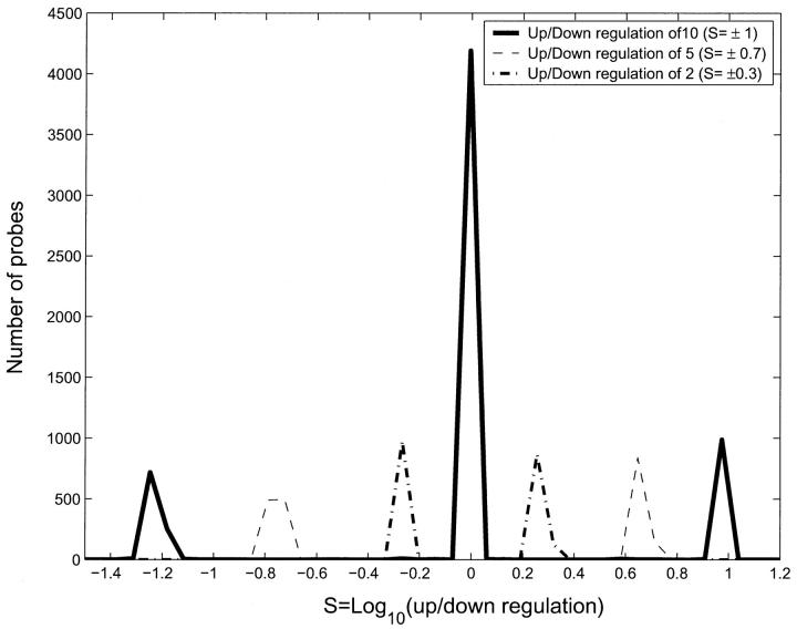
Fig. 9 shows a histogram of S for the three experiments. The outermost peaks correspond to f = 10, followed by f = 5 and f = 2, which are closest to the center. The central peak has probes that bind to targets with the same concentration as the control. From this figure, the thresholds to use for different levels of sensitivity in target concentration can be read off. For instance, if one could measure S in the range |S| > 1.1 then one would be able to measure upregulation by a factor of 10 but not downregulation by the same factor. This shift is due to the bias toward upregulation compared to downregulation mentioned previously. This bias, although much decreased in the OPS, is not entirely eliminated.

FIGURE 9.

Histogram of number of probes as a function of S for OPS. 4213 probes were not regulated and have S values close to 0. In each experiment 1000 probes were upregulated and 1000 probes were downregulated. Probes which were up-/downregulated by a factor of 10 have S values of ± 1. Probes which were up-/downregulated by a factor of 5 have S values of ± log₁0(5) and so on. The correlation between the up-/downregulation of the targets and the value of S is clear from the figure. This excellent correlation comes from the probe selection algorithm, which select probes for an optimal specificity. Note the bias toward upregulated genes. If the experimental sensitivity is |S| > 1.1 then we will be able to measure upregulation by a factor of 10 but not downregulation by the same factor. This is a residue of the concentration-dependent bias discussed in the text, which is reduced but not eliminated for the OPS.

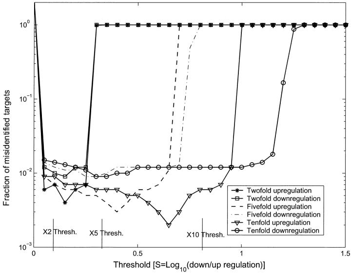
The number and identity of the targets that were up-/downregulated can be computed from Fig. 9 and compared with their correct values to estimate the error. We find that even with the OPS, with a precise knowledge of the target concentrations in the control and up-/downregulation by discrete factors, there is a small statistical error. We show in Fig. 10 the total fraction of misidentified targets (number of false-positives + number of false-negatives) as a function of threshold (S value). This is computed as follows. We know which targets were up- and downregulated. For each value S_t of the threshold in S, we count how many probes have value S > S_t and how many have S < −S_t. Those in the first set we identify as representing targets that are upregulated and those in the second set as representing targets that are downregulated. Comparing these sets to the actual up- and downregulated targets yields the total number identified in error. Clearly, the error is 100% when S_t is big enough. As S_t is lowered below the level where the signal for the up-/downregulated targets begins, the error will decrease as more and more targets are identified correctly. However, when S_t is decreased below the point where all up-/downregulated targets are identified, it will increase again because we will start including targets as up-/downregulated because of statistical fluctuation. Thus, the minima in the error for up-/downregulation by factors of 10, 5, and 2 in Fig. 10 represent the optimum thresholds for these regulation values. Note that the minima for upregulation are deeper than those for downregulation for each f. This means, as we have already noted, that upregulation is more accurately measured than downregulation for any fixed t.

FIGURE 10.

Fraction of misidentified targets for different thresholds (S_t), for the f = 10, f = 5 and f = 2 simulations. If the targets were regulated so that their |S| value was smaller than S_t, then they would be completely misidentified. Thus for large S_t the fractional error is unity. As the threshold S_t is lowered from large values, we measure various regulation levels from large to small. This is indicated in the figure by the different error levels for our experimental regulation levels dropping as their threshold is crossed. Notice however, that if we use S_t as a measure of the actual regulation level, then upregulation levels are measured more accurately (i.e., they are measured almost at their correct value of S_t) than downregulation levels (the S_t value for which would suggest a greater downregulation than is actually present). Even when the threshold is lower than the up-/downregulation level cutoffs (marked in the figure with vertical lines), there are still a small fraction (0.1–1%) of misidentified targets from statistical fluctuations.

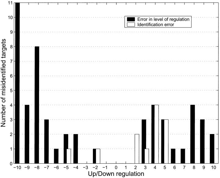
Finally, we did a simulation where we up- and downregulated 1000 targets each but the amount of up-/downregulation was randomly set to an integer value between 2 and 10. We compared the up-/downregulated simulation to a control simulation at t = 50,000 s. We then binned the binding level ratios at the values corresponding to the integer regulation levels that we had chosen. Negative numbers represent downregulated targets; positive represent upregulated targets. The light bars in Fig. 11 show the error in identifying the number of up- or downregulated genes. The solid bars show the error in identifying whether an up- or downregulated gene was identified as such. The light bars are computed as the absolute value of the number of genes identified as up-/downregulated vs. the number actually up-/downregulated at any given level of regulation. The solid bars are computed by going over the list of up-/downregulated genes and counting how many were not identified as up-/downregulated. The figure clearly indicates that it is relatively simple to measure how many targets are up- or downregulated but significantly harder to find out precisely which ones. This is because the first error has two parts (x₁, x₂, say) which partially cancel. The two contributions to this error are: x₁ = those genes that were identified as regulated but in fact were not and x₂ = those genes which were regulated but not identified as such. The light bars plot the quantity x₃ = abs(x₁−x₂). The solid bars on the other hand, plot the error in identifying the genes that are regulated, which is just x₂ and which is always greater than x₃.

FIGURE 11.

Number of up-/downregulated targets as a function of S for an experiment where 1000 targets each were up-/downregulated by known integer amounts randomly in [2,10]. Positive integers refer to upregulation, negative to downregulation. The light bars show the identification error, which is the number of targets that are incorrectly identified as up- or downregulated. This is computed as the absolute value of (the number identified as up-/downregulated vs. the number actually up-/downregulated) at any given level of regulation. The solid bars show the error in identifying the precise regulation level (amount of regulation) of the targets that were up-/downregulated. This is computed by going over the list of up-/downregulated genes and counting how many were not identified as up-/downregulated. The figure clearly indicates that it is relatively simple to measure how many targets are up- or downregulated but significantly harder to find out precisely which ones. This is because the first error has two parts (x1, x2, say) which partially cancel. The two contributions to this error are: x₁ = those genes that were identified as regulated but in fact were not, and x₂ = those genes which were regulated but not identified as such. The error in identifying how many genes were regulated is x₃ = abs(x₁−x₂). On the other hand, the error in identifying the genes that are regulated is just x₂ which is always greater than x₃. Further, the figure also shows that this problem is more severe for downregulated targets than for upregulated targets.

As in the previous figure, the error in identifying how many targets are up- or downregulated is small and depends on how sensitive a criterion one wants to impose. The error in computing the actual regulation level is greater (5–10% for our choice of binning) and worse for downregulated targets than for upregulated targets. This error can be separated into an error resulting from stochastic noise, and error occurring due to the low level of cross-binding still present in our probe set and the fact that for finite time there is a small bias toward measuring upregulation. To resolve this error we ran the simulation five times, keeping the up- and downregulations identical over the target set but changing only the random number seed. The averaging over these runs significantly reduced the error in computing the regulation level but had no effect on the error in identifying the number of up-/downregulated targets. We conclude that the error in computing the number of up-/downregulated targets is due to cross-binding although the error in computing the amount of regulation is stochastic. To validate this, we reran the simulation with no cross-binding, but with the stochastic noise unchanged. As expected, in this simulation there were no identification errors, but the level of error in determining the exact amount of regulation was still present.

DISCUSSION AND CONCLUSIONS

We have described a general method of computer simulations to model the hybridization kinetics of gene arrays. Such computer modeling allows one to quickly isolate the experimental conditions that affect the accuracy of such gene array experiments. In this article, we use the yeast genome and two different probe sets. One of these sets (RPS) was created by selecting a random 25-mer sequence from each gene whereas the other (OPS) was created by choosing those 25-mers from each gene which would minimize cross-binding to all other genes. We consider our method to select such an optimized probe set, which minimizes crosshybridization while retaining gene specificity, as one of the major results of this article.

Using the RPS and OPS, we studied the dynamics of the hybridization process by computer simulation. We first analyzed the RPS to study the effects of crosshybridization, diffusion, and target concentration. We found that for the RPS, the fact that many probes bind to a given target, results in unacceptably high levels of crosshybridization (Fig. 4) which prevent reaching an equilibrium distribution. Next (Fig. 5), by comparing finite diffusion with instantaneous diffusion, we showed that the diffusion coefficient is large enough not to pose any essential problem. This is partly due to the fact that our targets are small, For larger targets, we expect diffusion to play a bigger role which may require other protocols, such as stirring or thermal annealing during hybridization, to reach an equilibrium distribution.

Finally (Figs. 6 and 7), by studying three different target concentration levels, we showed that after 50,000 s, which is the typical hybridization time in a gene-array experiment, there is a significant effect of target concentration. Targets that have a high concentration level are closer to equilibrium (have a greater fraction bound to correct target) than targets that have a low concentration level. This suggests a serious systematic bias in real experimental situations. In any experiment run for a finite time, downregulated gene levels would be measured lower than their actual downregulation and upregulated gene levels would be measured higher than their actual upregulation levels.

For the OPS, where the crosshybridization is very low, the problems from target concentration effects are less severe (Fig. 8), although they are not completely eliminated. To study these effects in more detail, we conducted a series of computer experiments (Figs. 9–11) on the OPS. We up-/downregulated targets by different amounts and attempted to identify both the targets that were up-/downregulated as well as their level of regulation. This was done by looking at their hybridization level compared to the baseline (unregulated) targets after 50,000 s of simulation.

These experiments confirmed our observation that downregulation is undermeasured and upregulation is overmeasured. Additionally, we found that it is very difficult to measure small variations in target regulation. In other words, for any set of experimental parameters (temperature, target size, probe set choice, hybridization time), there is some value of regulation below which it is impossible to measure regulation because the error rate is too large. This error has two components. One is the error in determining the number of up- or downregulated genes. The other is the error in identifying precisely which gene was up- or downregulated. The first error is significantly smaller than the second (Fig. 11). Thus, one can measure the number of genes which are up-/downregulated by a certain amount much more accurately than one can identify which genes they are.

Gene arrays are being used for an extraordinary range of applications that affect humans directly. These include cancer identification and staging, identifying individuals at risk for genetic disorders, drug regimens specific to the genetic signature of patients, etc. They have also become almost ubiquitous tools in pharmaceutical companies and research labs. It is therefore important to be able to determine the accuracy of the results of such gene array experiments. We view our computer experiment as a first step in this direction. It provides a relatively inexpensive and accurate method for studying the kinetics of gene array experiments to optimize parameter values and experimental protocols for more accurate predictions. Our methods can clearly be generalized to other genomes and experimental situations, such as more complex gene arrays, more sophisticated data collection methods, other parameter values, annealing, washing and stirring protocols, and so on.

Gene array experiments are ever more widely used. It is necessary that their results be validated by some process which has a high degree of credibility. We believe that computer simulations, if they were sufficiently detailed, could play this role. It is our hope that such computer modeling will become an integral part of the validation process of gene array results. We have devised a simulation tool, which may be used to plan experiments and validate their results.

References

- Chan, V., D. J. Graves, and S. E. McKenzie. 1995. The biophysics of DNA hybridization with immobilized oligonucleotide probes. Biophys. J. 69:2243–2255. [DOI] [PMC free article] [PubMed] [Google Scholar]
- DeRisi, J., L. Penland, P. O. Brown, M. L. Bittner, P. S. Meltzer, M. Ray, Y. Chen, Y. A. Su, and J. M. Trent. 1996. Use of a cDNA microarray to analyse gene expression patterns in human cancer. Nat. Genet. 14:457–460. [DOI] [PubMed] [Google Scholar]
- Duggan, D. J., M. Bittner, Y. Chen, P. Meltzer, and J. M. Trent. 1999. Expression profiling using cDNA microarrays. Nat. Genet. 21:10–14 (Suppl.). [DOI] [PubMed] [Google Scholar]
- Eisen, M. B., P. T. Spellman, P. O. Brown, and D. Biostein. 1998. Cluster analysis and display of genome-wide expression data. Proc. Natl. Acad. Sci. USA. 95:14863–14868. [DOI] [PMC free article] [PubMed] [Google Scholar]
- Fotin, A. V., and A. D. Mirzabekov. 1998. Parallel thermodynamic analysis of duplexes on oligonucleotide microchips. Nucleic Acids Res. 26:1515–1521. [DOI] [PMC free article] [PubMed] [Google Scholar]
- Hughes, T. R., M. Mao, A. R. Jones, J. Burchard, M. J. Marton, K. W. Shannon, S. M. Lefkowitz, M. Ziman, J. M. Schelter, M. R. Meyer, S. Kobayashi, C. Davis, H. Dai, Y. D. He, S. B. Stephaniants, G. Cavet, W. L. Walker, A. West, E. Coffey, D. D. Shoemaker, R. Stoughton, A. P. Blanchard, S. H. Friend, and P. S. Linsley. 2001. Expression profiling using microarrays fabricated by an ink-jet oligonucleotide synthesizer. Nat. Biotechnol. 19:342–347. [DOI] [PubMed] [Google Scholar]
- Lashkari, D. A., J. L. DeRisi, J. H. McCusker, A. F. Namath, C. Gentile, S. Y. Hwang, P. O. Brown, and R. W. Davis. 1997. Yeast microarrays for genome wide parallel genetic and gene expression analysis. Proc. Natl. Acad. Sci. USA. 94:13057–13062. [DOI] [PMC free article] [PubMed] [Google Scholar]
- LeProust, E., J. P. Pellois, P. Yu, H. Zhang, X. Gao, O. Srivannavit, E. Gulari, and X. Zhou. 2000. Digital light-directed synthesis. A microarray platform that permits rapid reaction optimization on a combinatorial basis. J. Comb. Chem. 2:349–354. [DOI] [PubMed] [Google Scholar]
- Li, F., and G. D. Stormo. 2001. Selection of optimal DNA oligos for gene expression arrays. Bioinformatics. 17:1067–1076. [DOI] [PubMed] [Google Scholar]
- Lipshutz, R. J., S. P. A. Fodor, T. R. Gingeras, and D. J. Lockhart. 1999. High density oligonucleotide arrays. Nat. Genet. 21:20–24 (Suppl.). [DOI] [PubMed] [Google Scholar]
- Lockhart, D., H. Dong, M. Byrne, M. Follettie, M. Gallo, M. Chee, M. Mittmann, C. Wang, M. Kobayashi, H. Horton, and E. Brown. 1996. Expression monitoring by hybridization to high-density oligonucleotide arrays. Nat. Biotechnol. 14:1675–1680. [DOI] [PubMed] [Google Scholar]
- SantaLucia, J. J. 1998. A unified view of polymer, dumbbell and oligonucleotide DNA nearest-neighbor thermodynamics. Proc. Natl. Acad. Sci. USA. 95:1460–1465. [DOI] [PMC free article] [PubMed] [Google Scholar]
- Schena, M., R. A. Heller, T. P. Theriault, K. Konrad, E. Lachenmeier, and R. W. Davis. 1998. Microarrays: biotechnology's discovery platform for functional genomics. Trends Biotechnol. 16:301–306. [DOI] [PubMed] [Google Scholar]
- Seneviratne, P. N., H. T. Allawi, and J. J. SantaLucia. 1999. Nearest neighbor thermodynamics of NMR of DNA sequences with internal AA, CC, GG and TT mismatches. Biochemistry. 38:3468–3477. [DOI] [PubMed] [Google Scholar]
- Singh-Gasson, S., R. D. Green, Y. Yue, C. Nelson, F. Blattner, M. R. Sussman, and F. Cerrina. 1999. Maskless fabrication of light-directed oligonucleotide microarrays using a digital micromirror array. Nat. Biotechnol. 17:974–978. [DOI] [PubMed] [Google Scholar]