Multiplexed-Replica Exchange Molecular Dynamics Method for Protein Folding Simulation

Abstract

Simulating protein folding thermodynamics starting purely from a protein sequence is a grand challenge of computational biology. Here, we present an algorithm to calculate a canonical distribution from molecular dynamics simulation of protein folding. This algorithm is based on the replica exchange method where the kinetic trapping problem is overcome by exchanging noninteracting replicas simulated at different temperatures. Our algorithm uses multiplexed-replicas with a number of independent molecular dynamics runs at each temperature. Exchanges of configurations between these multiplexed-replicas are also tried, rendering the algorithm applicable to large-scale distributed computing (i.e., highly heterogeneous parallel computers with processors having different computational power). We demonstrate the enhanced sampling of this algorithm by simulating the folding thermodynamics of a 23 amino acid miniprotein. We show that better convergence is achieved compared to constant temperature molecular dynamics simulation, with an efficient scaling to large number of computer processors. Indeed, this enhanced sampling results in (to our knowledge) the first example of a replica exchange algorithm that samples a folded structure starting from a completely unfolded state.

INTRODUCTION

In a molecular dynamics (MD) simulation study of thermodynamics, a representative sampling over the entire phase space is needed to obtain an accurate canonical distribution at a given temperature. For large molecules such as proteins, this sampling is usually difficult, especially at physiological temperature, because molecules tend to be trapped in a large number of local energy minima, which slows the sampling of phase space.

Recently, a number of attempts have been made to overcome this kinetic trapping problem (Berg and Neuhaus, 1991; Berg and Neuhaus, 1992; Hansmann, 1997; Hansmann and Okamoto, 1993; Hao and Scheraga, 1994; Mitsutake et al., 2001; Nakajima et al., 1997; Torrie and Valleau, 1977). One successful method is replica exchange molecular dynamics (REMD). The replica exchange method was developed first in the physics community to improve sampling in glassy systems (Hukushima and Nemoto, 1996; Shirakura and Matsubara, 1996), and has been recently applied to an MD simulation of biomolecules by Sugita and Okamoto (1999) and later by García and co-workers (García and Sanbonmatsu, 2001; Sanbonmatsu and García, 2002). In this method, a number of simulations are performed at different temperatures in parallel, and exchanges of configurations are tried periodically. Even if a trajectory is temporarily trapped in a local minimum, the simulation can escape from this minimum via an exchange with a higher temperature configuration. With this method, one can obtain various thermodynamic quantities as a function of temperature for a wide temperature range from a single simulation run. Moreover, because each replica can be simulated using its own computer processor, the REMD method is well suited for and very efficiently runs on parallel computers, which have become ubiquitous in recent years.

However, there are two aspects to REMD that have limited its ability to gain better thermodynamic sampling. First, REMD can only be efficiently realized with a homogeneous parallel machine (or a homogeneous parallel cluster of computers), where the performance of all processors is comparable. Because an REMD calculation requires synchronization between processors to facilitate the exchanges between replicas, the slowest replica determines the overall progress of the MD simulation and it becomes important to use processors with the same speed. Therefore, REMD is not suitable for a heterogeneous parallel system such as a large-scale distributed computing (e.g., Folding@home (Shirts and Pande, 2001b)). Second, the REMD method only scales efficiently to tens of processors, inasmuch as each temperature replica uses only one processor. One might be tempted to efficiently scale to large processor clusters (and thus achieve better sampling) simply by adding more replicas. However, because efficient sampling requires diffusion in temperature replica space (Sugita and Okamoto, 1999), adding more temperature replicas means that the number of swaps grows quadratically and that either longer simulations are needed (which requires more CPU time) or exchanges must be attempted more frequently (which typically requires faster communication between processors). These limitations are significant due to both the growing use of heterogeneous clusters of PCs (either in worldwide distributed computing or smaller-scale calculations) as a computational platform for any scale of calculation, as well as the great computational potential of thousands to millions of processors that large-scale distributed computing may provide.

In this paper, we present our modified approach to the REMD method. Multiple replicas are used for each temperature level and exchanges between these replicas are also tried, eliminating the synchronization needed in the original REMD method. This multiplexed-replica exchange molecular dynamics (MREMD) method is tested with a small model protein (BBA5) starting from a fully unfolded state. With large-scale distributed computing, we have simulated more than 200 microseconds of aggregate atomistic molecular dynamics simulation time, allowing our simulation to reach the folded state of BBA5 starting from the unfolded state (a first for REMD-based simulation). By comparing it with a constant temperature simulation, it is shown that the present method can achieve an appropriate sampling of the configuration space in a shorter simulation time. We also discuss the limitations of our method.

METHODS

Replica exchange molecular dynamics

Details of the REMD algorithm are described elsewhere (Sugita and Okamoto, 1999). For completeness and comparisons to MREMD, we briefly describe the REMD method. In REMD, regular MD runs are started from a set of n independent configurations at corresponding temperatures at time 0. After a certain amount of integration time, a new set of configurations is obtained as . At this time, an exchange of configurations and is tried with a Metropolis criterion

(1)

This acceptance probability ensures the detailed balance condition of the overall Monte Carlo process. These simple two steps are repeated and an average of a thermodynamic property A at temperature is obtained from an average

(2)

This procedure can be considered as a Markov process with two operators. Namely, if we define the MD operator M as one that generates the result of MD simulation with the given time step, and swap operator S as another that swaps two configurations with the above probability given in Eq. 1, a thermodynamic property can be obtained with a Markov chain determined with

(3)

In practice, exchanges between adjacent temperature levels are tried (namely, or in Eq. 1) to increase the acceptance ratio. Also, a number of swaps (up to n/2) can be tried after each MD run.

Multiplexed-replica exchange molecular dynamics

Instead of using one replica for each temperature, we have multiplexed the replica in each temperature by M-times. Accordingly, we have for corresponding temperatures with

(4)

at time 0. To distinguish replicas within one temperature level from those with different temperatures, let us denote them as multiplexed-replicas. In other words, there are M multiplexed-replicas in each set . We can extend our definition of MD and swap operators such that they can act on . Now, let us suppose a rearrangement operator , which rearranges the multiplexed-replicas within the i-th temperature level in an arbitrary order. Namely,

(5)

where is an arbitrary rearrangement of . Because rearranges configurations within the same temperature, applying it to the Monte Carlo process generates another Markov chain. Namely, a Markov chain determined with

(6)

gives a correct thermodynamic property when averaged over all multiplexed-replicas:

(7)

Here, is a rearrangement operator over all temperature levels defined as

(8)

This process is schematically illustrated in Fig. 1 together with the original REMD. In MREMD, it can be considered that there are M multiplexed-replica “layers,” each of which has n different temperature levels. After each MD step, exchanges between replicas in different layers are tried as well as exchanges between regular replicas in the same layer.

FIGURE 1.

Schematic illustrations of a REMD and b MREMD method with five replicas. M = 2 is used for MREMD for simplicity.

Even though any arbitrary rearrangement is acceptable mathematically, we must be careful in practice in how we schedule simulations when using a cluster with different processor speeds to achieve the greatest performance of the cluster. In particular, the rearrangement of multiplexed-replicas is conducted in such a way that the simulations in the multiplexed-replica layers are scheduled to be completed from the top layer as simulations in each temperature level are completed. The configuration completed first in one temperature level is sent to the first layer, and following configurations are sent to the next layers in the order of completion. This rearrangement greatly enhances the efficiency of the method on heterogeneous clusters.

The efficiency enhancement arises from the following. Before an exchange of configurations can be tried, there will always be some processor idling time, the length of which is mainly determined by the nature of the processors in the system. Namely, for any exchange pair, simulation on the configuration completed earlier must wait until the second is completed. In a regular REMD method, each configuration is paired to only one other configuration. In MREMD method, on the other hand, any configuration can be exchanged with M multiplexed-replicas. By rearranging multiplexed-replicas, it becomes possible to minimize the total idling time. Also, the idling time becomes negligible compared to the total simulation time if a large number of multiplexed-replicas are used.

Furthermore, we expect that the additional simulations used in the multiplexing at each temperature level should also enhance sampling. Consider M replicas running at the same temperature. Because folding of small proteins generally follows single exponential kinetics, one can efficiently speed the sampling of folding simulations by performing many independent simulations. Indeed, we expect the fraction that fold in time t to be , where k is the folding rate. From 1000 independent simulations of a fast folding protein with k ∼ 1/5000 ns, we expect 1000 simulations × 50 ns/5000 ns = 10 simulations to fold. Thus, because additional simulations can also aid the sampling and lead to the folded state, the MREMD method takes advantage of both the multiple temperature aspect of REMD as well as a large number of independent simulations to considerably enhance sampling as compared to either method alone.

Computation

The method presented above was applied to the folding simulation of the 23-amino acid model protein BBA5 with the capped sequence Ace-YRVPSYDFSRSDELAKLLRQHAG-NH₂. BBA5 was modeled using the OPLS united atom parameter set (Jorgensen and Tirado-Rives, 1988) and Still's GB/SA implicit solvent model (Qiu et al., 1997) in our modified version of the TINKER molecular dynamics simulation package (http://dasher.wustl.edu/tinker/) within Folding@home (Shirts and Pande, 2001b). Langevin dynamics with Allen's stochastic integrator (Allen, 1980; Allen and Tildesley, 1987) was used to simulate the viscous drag of water (γ = 91 ps⁻¹) and bond lengths were constrained using RATTLE algorithm (Andersen, 1983) allowing 2 fs of time step. For electrostatic calculations, 16 Å cutoffs and 12 Å tapers were employed. MREMD exchanges of configurations were attempted every 1 ns and trajectories were integrated up to 50 ns, leading to the total aggregate simulation time of 10 μs for each temperature level. The simulation time between configuration exchanges is relatively long compared to the one adopted by previous investigators (Sanbonmatsu and García, 2002; Zhou et al., 2001). The benefit of longer times between exchanges is the possibility of greater decorrelation of the simulations between exchange attempts. The principal disadvantage is that we must use more closely spaced temperature levels to enable exchanges with high acceptance ratios. To that end, we employed 20 exponentially distributed temperatures between 250 and 500 K with 200 multiplexed-replicas in each level. A fully extended structure with angles (ϕ, ψ) = (−135°, 135°) for all amino acids was generated and then equilibrated with 100 ps of molecular dynamics step. This stabilized structure was used for all 4000 starting configurations. The simulation was performed on a supercluster of processors distributed worldwide, with the total number of processors scaling to tens of thousands (Shirts and Pande, 2001b).

Structural characterization of the BBA5 requires the native structure of the peptide. For this purpose, an NMR structure was taken (Struthers et al., 1998) and then stabilized by performing 10 steps of BFGS quasi-Newton energy minimization (Fletcher, 1987) followed by 100 ps of molecular dynamics simulation at 279 K. Secondary structure was determined using the program DSSP (Kabsch and Sander, 1983) with the default hydrogen bond cutoff parameter of 0.5 kcal/mol. α-helices were found by searching for conformations containing at least four consecutive helical residues according to this program. β-hairpins were found by searching β-bridges between residues 2-7 and 3-6. To find conformations with correct tertiary structure, the α-carbon root-mean-square distance (RMSD_α) with respect to the native structure was calculated using an efficient geometry alignment algorithm (Rhee, 2000). A conformation was declared to be folded if it contained both the helix and the hairpin, and had RMSD_α below 3.6 Å.

RESULTS AND DISCUSSION

Replica exchange diagnostics

Because the advantage of the MREMD method arises from the exchanges of configurations between different temperatures, it is vital to use temperatures that allow a significant number of such exchanges. Fig. 2 a shows the probability distributions of potential energy at each temperature level using configurations obtained after 10 ns of simulation time. By discarding the initial 10-ns data for each replica, we eliminated the unrealistic high energy populations caused by the memory of the fully extended starting configuration. From this figure we can see that any two distributions with adjacent temperatures show a significant overlap. As a result, a high fraction of exchange trials was accepted with the ratio reaching up to 65% over the entire temperature range. The extent of exchanges in temperature space is illustrated in Fig. 2 b. Here, the temperature indices are followed for 20 different trajectories started from the first multiplexed-replica layer. All other trajectories show similar exchange patterns. From this figure, it is also clear that any trajectory visits nearly all temperature levels within the simulation time. To verify that these exchanges lead to a desirable sampling over the potential energy space, we have also examined the ratio of the potential energy distributions of adjacent temperatures. If the potential energy distribution functions and follow the Boltzmann distribution, their ratio will satisfy

(9)

FIGURE 2.

(a) Probability distributions of potential energy at all temperature levels obtained with MREMD method. Configurations obtained after 10 ns are used to generate the distribution. The leftmost one represents the 250 K result. The temperature rises as it goes to the right. (b) Exchanges of replicas in the temperature space; drawn by following temperature indices of 20 example configurations, each of which was started from a different temperature level. (c) Ratios of probabilities with adjacent temperatures.

A plot of this ratio is shown in Fig. 2 c. For all temperatures, satisfactory linearity is observed, suggesting that the configurations from our simulation follow the Boltzmann distribution.

Comparison with the constant temperature simulation

Experimentally, BBA5 was found to have a well-defined α-helix and a β-hairpin in its native state (Struthers et al., 1998). Because we have started simulations from a fully extended (i.e., completely nonnative) configuration for all the replicas, an inspection of trajectories reaching the folded state reveals the extent to which the simulation samples the available configuration space. Fig. 3 shows the stereo representation of a folded conformation obtained with the simulation, together with the experimentally determined native structure. Overall, the conformation reached by simulation shows a good agreement with experiment with well-defined secondary structure. To represent the time variation of structural features, snapshots of three arbitrarily chosen folding trajectories are illustrated in Fig. 4. The variations of potential energy and RMSD_α of these trajectories are also presented in Fig. 5. From a comparison with Fig. 2, it can be inferred that the potential energy values sampled by these folding trajectories contribute to low energy population in the distribution. It is also clear that these trajectories reach the folded state characterized by well-defined secondary structure and low RMSD_α. Because we observe a large number of such trajectories (∼100), we conclude that our simulation has sampled the folded state region of the configuration space within a relatively short simulation time.

FIGURE 3.

Stereo representations of (a) a folded conformation example and (b) the native structure. For simplicity, only C_α backbone and selected side chains (Val3, Phe8, Leu14, Leu17, and Lue18) are shown. The β-hairpin (residues 2-7) and the α-helix (residues 12-20) regions are represented in blue and red, respectively.

FIGURE 4.

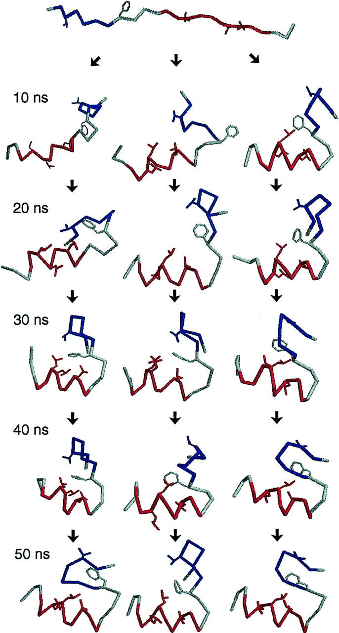
Snapshots of three selected folding trajectories obtained at every 10-ns simulation time. The same coloring scheme in Fig. 3 is adopted.

FIGURE 5.

Evolution of RMSD_α (solid lines) and the potential energy (dotted lines) of the selected folding trajectories.

In addition, the number of trajectories with such well-defined native-like structure will increase in time because we started the simulation from a fully unfolded state as described above. The primary reason to use an REMD-like method is the hope that REMD will speed sampling. To this end, we can calculate the rate of structure formation using REMD and compare it directly to non-REMD enhanced, constant temperature methods. Although the “rate” of folding obtained from an REMD simulation cannot be compared with experiment (because the exchanges in temperature space destroys the kinetic information), this REMD rate can still be used as a useful measure to estimate its effectiveness over the constant temperature molecular dynamics (CTMD). Indeed, if MREMD speeds sampling, we would expect the MREMD folding rate to be faster than that of CTMD. Moreover, a comparison of the MREMD rate with CTMD allows one to quantitatively evaluate the enhancement of sampling gained by MREMD.

For the purpose of the comparison of MREMD and CTMD, we compare our MREMD results with a CTMD simulation performed with 200 independent trajectories of 50 ns each at a relatively low temperature (279 K). Fig. 6 shows the time evolution of the fractions of configurations containing the α-helix and β-hairpin secondary structures at the same temperature for both MREMD and CTMD methods together with the average RMSD_α. For both of the secondary structure elements, one can see that MREMD shows faster population growth through the overall simulation time. Time evolution of the average RMSD_α shows a similar result. As a consequence, we can conclude that the MREMD method enables a considerable speedup for the search in configuration space. Namely, whereas a trajectory in CTMD spends a significant amount of time in local minima, a trajectory in MREMD method easily escapes from such states by exchanging configurations from different temperatures. This trapping effect can be clearly visualized by comparing the potential energy distributions obtained with both methods; because configurations trapped in local minima will contribute to high energy population, the potential energy distribution from CTMD will display a shift toward a high energy direction unless the simulation time is long enough. Fig. 7 compares the potential energy distribution obtained with CTMD with one from MREMD. One can clearly see that the energy distribution from CTMD shows the expected shift.

FIGURE 6.

Evolutions of populations with native-like characters: (a) α-helix, (b) β-turn; (c) evolution of the average RMSD_α. Solid lines represent the results at 279 K of temperature obtained with MREMD method. Dotted lines represent the results from CTMD method at the same temperature.

FIGURE 7.

Probability distributions of potential energy at 279 K from MREMD (solid line) and CTMD (dotted line) methods.

Because a massive number (tens of thousands) of trajectories have been simulated in this study, we have observed a considerable fraction of trajectories reaching the folded state within the 50-ns simulation time (per processor, for a total of 200 μs). To estimate the speedup by MREMD in a more quantitative manner (and to test how MREMD enhances the sampling of the native state), the ensemble dynamics method (Shirts and Pande, 2001a; Zagrovic et al., 2001) was applied where the folding rate k is estimated from the probability distribution for folding event

(10)

Here, M is the total number of independent ensembles, or the number of multiplexed-replicas in one temperature level. When t is close to zero, this ratio shows a linear relationship and the folding rate can be approximated as . The estimated folding time constants () at 279 K for MREMD and CTMD were found to be 0.97 μs and 6.4 μs, respectively. Although the rates and kinetics resulting from MREMD are devoid of a physical meaning as mentioned earlier, this difference demonstrates that the MREMD with replica-exchange trial frequency of once per 1 ns speeds the search in the configuration space with approximately an order of magnitude difference.

One possible concern here may be the degree of agreement between the structure of the native states dictated by the theoretical model and the experiment. Namely, assuming that the experimental structure is unstable or metastable on the forcefield adopted in the simulation, it can be argued that the search may have only reached this native-like conformation without truly accessing the most stable free energy minimum. From the fact that the potential energy values of the “folded conformation” is usually on the low energy side of the distribution shown in Fig. 2, we speculate that this will be rather implausible, even though we cannot ascertain it at this stage because the stability is determined by free energy rather than the potential. To verify the stability of the experimental native structure on the forcefield, it is necessary to perform a simulation starting directly from this structure. This will be discussed in the following section.

Sampling of the configuration space: comparison with an unfolding simulation

Suppose that the experimentally determined native structure is unstable on the forcefield adopted in the simulation. Then, the majority of trajectories will lose structural features if we perform a number of simulations starting from this native structure. (Henceforth, the simulation started from the extended state will be denoted as the run started unfolded, whereas the simulation started from the native state will be denoted as the run started folded.) Therefore, the run started folded can be used to manifest the stability of the experimental native structure on the forcefield. We have performed the same MREMD simulation from the native structure. From an ensemble of 10,000 configurations (200 multiplexed-replicas with 50-ns simulation with configurations sampled each nanosecond) obtained at 300 K, we have obtained a representative conformation by calculating the distance matrix for each member of the ensemble, averaging this matrix over the ensemble, and then finding the structure that most closely resembles the ensemble averaged distance matrix (Zagrovic et al., 2002). Fig. 8 shows the stereo representation of this configuration, which presents a remarkable resemblance to the native structure in Fig. 3. Moreover, both the α-helix and β-hairpin were found to be intact in most of the trajectories (>65%) at low temperatures (<350 K). Accordingly, we may safely assume that the native structure is stable in the forcefield adopted in this work.

FIGURE 8.

Stereo representation of a representative conformation from the unfolding simulation.

Perhaps the most important advantage of this supplemental simulation is the fact that its result can be used to examine the convergence of the MREMD method. Although we have observed a significant speedup using MREMD instead of CTMD, this does not imply that the configurations sampled during the simulation represent the entire available space for this model protein. In fact, convergence to the thermodynamically correct equilibrium is the most demanding objective to accomplish in a simulation of a large molecule. In principle, a sufficient sampling requires the trajectories to visit the entire range of the available configuration space, and will be accompanied by a full loss of memory of the initial conditions. Accordingly, if we can observe the same convergence from two independent simulations started from fairly different configurations, i.e., from both runs started unfolded and folded, the method will be more reliable in terms of sampling of the configuration space. To precisely monitor the convergence, it is useful to survey the time variation of thermodynamic properties. To this end, the free energy distribution, or the potential of mean force (Leach, 2001) as a function of RMSD_α and the radius of gyration of the entire peptide (R_g)

(11)

has been monitored. The principal component method (García, 1992) was not used in this study, as the principal component basis vectors from the runs started unfolded and folded, obtained with all sampled configurations in each case, will likely have different physical implications. Instead, it is more direct to use the well-understood degrees of freedom RMSD_α and R_g.

Fig. 9 shows the free energy contour maps obtained from the runs started unfolded and folded at various temperatures. It also shows the difference of the free energy patterns from both simulations. It can be clearly seen that free energy patterns from both runs become more similar with longer simulation time. One striking feature to note is that even though the free energy pattern is converging, a satisfactory convergence within 50 ns of simulation time has been reached only in the high temperature (500 K) case. To facilitate a direct comparison, one-dimensional free energy versus RMSD_α and the potential energy at 300 K of temperature is plotted in Fig. 10.

FIGURE 9.

Time evolution of free energy contour maps versus RMSD_α and R_g at (a) 250 K, (b) 300 K, (c) 402 K, and (d) 500 K. From the left, each column represents the distributions obtained from the run started unfolded, the run started folded, and the difference, respectively. From the top, each row is based on configurations obtained during 0 ∼ 10-ns, 20 ∼ 30-ns, and 40 ∼ 50-ns simulation time windows, respectively. Color code is explained in the inset at the bottom. Free energy is in k_BT unit.

FIGURE 10.

One-dimensional free energy profiles from the run started unfolded (solid lines) and the run started folded (dotted lines) as a function of (a) RMSD_α and (b) the potential energy at 300 K. For visual clarity, curves are shifted down from each other by 7 k_BT.

The discrepancy between the results from the runs started unfolded and folded suggests an important precaution and limitation for the application of the replica exchange method. Even when the potential energy distribution displays a correct Boltzmann distribution as shown in Fig. 2 c, it is possible that the sampling over the configuration space is not sufficient. This is especially important in the replica exchange method because what is pursued in this type of simulation is thermodynamically reliable information of the system with relatively short simulations per replica. This result is consistent with previous replica exchange simulations of proteins, because although Boltzmann sampling appears to be satisfied, no previous REMD simulation starting from an unfolded structure has reached the folded state, thus suggesting incomplete sampling. Our ability (using thousands of processors with MREMD) to reach the folded state starting from an unfolded configuration represents greater sampling, but clearly even this level of computation is insufficient for complete sampling of the phase space.

In principle, the speedup in a replica exchange method arises from the fact that a trajectory trapped in a local minimum can be forced to escape by exchanging configurations with a higher temperature simulation. However, the exchange itself is another important mechanism that can render faster convergence. Suppose we have a system with two local potential energy minima, or two states as shown in Fig. 11 a. If the degrees of freedom along a reaction coordinate in the two states are different from each other at any given energy, free energies of the two states will have different temperature dependences. Accordingly, the probability distribution along the coordinate will also be different at different temperatures. (See Fig. 11, b and c.) Now suppose that one performs a simulation with two replicas starting from each potential energy minimum point. Within a very short simulation time, one will observe a significant speedup over a single simulation started from one state because any exchange will cause each trajectory to sample both states. Namely, because both of the states cannot be reached within that short simulation time in a regular single simulation, the sampling with the exchange method will appear to be considerably improved. Nevertheless, the probability distribution with this short simulation at one temperature will be strongly correlated to the distribution at the other temperature. In this two-state case, for example, the probability distributions will be complementary to each other as shown in Fig. 11 d. Therefore, we can infer that it is not possible to obtain correct probability distributions for both temperatures only with such exchanges. As the simulation time is lengthened, the trajectory started from one state will visit the other state and this complementariness will be removed. Consequently, one can conclude that the simulation time should be long enough such that each trajectory can cover the entire configuration space as well as the entire temperature space to overcome this fictitious speedup. In fact, this is why it is not feasible to decrease the necessary simulation time by simultaneously performing a multiple number of simulations starting from different configurations. Unless the initial configurations properly represent the entire configuration space of the system, thermodynamically acceptable results cannot be expected within relatively short simulation time.

FIGURE 11.

Schematic illustration of the fictitious speedup by configuration exchanges for a two-state system. (a) The potential energy of the system; (b) free energy at a high (solid line) and a low (dotted line) temperatures; (c) the correct probability distributions at the two temperatures; (d) an example of incorrect probability distributions obtained with a short replica exchange simulation, where the two distributions are complementary to each other.

Moreover, it is interesting to ask to what degree we expect exchange methods to speed sampling. To answer this question, one must formulate a model of the dynamics of exchange-based simulations, inasmuch as the rate of convergence and sampling is a kinetic phenomenon. Toward this end, consider a system with two states, unfolded (U) and folded (F) and with some temperature dependent rates of conversion and , respectively. In an exchange simulation, we also must consider the rate of exchange between replicas at different temperatures within a given state, i.e., and . The overall kinetics of the system will depend on both types of rates, as summarized in Fig. 12. With this system and the rates, our question is what is the new effective rate connecting states U and F at the temperature of interest (e.g., 300 K). Usually, the exchange rates between different replicas within a state are orders of magnitude faster than the conversion rates between different states. For example, whereas the conversion rates and are in the order of (10 μs)⁻¹ at 300 K for BBA5, the timescale of the exchanges is in nanoseconds in our case, and is typically faster in other exchange-based simulations. Therefore, it can be inferred that the overall rate is still determined by the slow conversion rates, even though we are using an exchange method for the very reason that the rate of crossing between U and F is very slow.

FIGURE 12.

Schematic illustration of an exchange simulation for a simple two-state system.

Next, we consider the effect of using replicas with elevated temperatures. For proteins at a very high temperature (e.g., 500 K), the folding rate is extremely slow (ms⁻¹ or slower) because the folded state (F) is thermodynamically unstable with very high free energy. (Because , where ΔG is the stability of the protein, and for high temperatures ΔG will be negative with a large magnitude, the folding rate will be very small.) Thus, simulations started from U will not be significantly sped toward F by exchanges. There will be some speed increase because there will likely be a rate maximum between 300 K and 500 K, and an exchange method will take full advantage of this. However, this increase will hardly be over an order of magnitude. On the other hand, the rate is fairly fast (ns⁻¹), and in simulations started from F, one would observe sampling of the unfolded state in a short simulation time. Nevertheless, the simulations will rarely refold in such a short time, and the sampling would be incomplete inasmuch as a thorough sampling is obtained when the memory of the initial condition is completely lost.

At this point, it will be pertinent to compare our results with previous replica exchange protein folding studies using much shorter simulation time in each replica. Sanbonmatsu and García (2002) studied the structural properties of five-residue peptide, Met-enkephalin with 16 temperature levels ranging from 275 K to 419 K. Simulations were conducted for 2 ns in each temperature level. By comparing configurations from all temperature levels with configurations obtained with a single 32-ns constant temperature simulation, they showed that the replica exchange method covered approximately five times larger configuration space. One interesting additional comparison that can be suggested for this system is to use 16 independent constant temperature runs starting from the same initial configurations used in replica exchange simulations. By comparing it with the single trajectory result, it may be possible to extract the aforementioned speedup effect. In our case, it should be pointed out that it is impossible to conduct such a comparison in the practical sense; the aggregate simulation time is ∼200 μs, and it will be extremely difficult to perform a single constant temperature simulation of this timescale.

Likewise, Zhou and co-workers reported replica exchange simulation results for the C-terminal 16-residue portion of protein G (Zhou et al., 2001). Using also 2 ns of simulation time for each of 64 replicas, they found that the resulting free energy contour surfaces showed noticeable ruggedness when plotted against overall RMSD and R_g. This is in qualitative agreement with the result reported by García and Sanbonmatsu (2001) for the same system with 3.5-ns simulation time and 32 replicas. However, it is in sharp contrast to Pande and co-workers' result obtained with a greater number of individual trajectories and longer simulation time (Zagrovic et al., 2001). This discrepancy may be attributed to the slow change of RMSD described previously. Assuming that the RMSD of this protein changes at a slow rate as in our system, it is highly probable that the contour map shows a clustered distribution around 64 initial configurations with only 2-ns simulation time. Also, this ruggedness may have been more pronounced than in the Met-enkephalin case (Sanbonmatsu and García, 2002), as an increase in the system size can slow the motion of the protein along RMSD.

CONCLUSIONS

Massively parallel clusters or “distributed computing” are becoming a significant computational paradigm for computational biology. Indeed, thousands to millions of processors can be harnessed to potentially break existing computational barriers. However, the efficient use of this resource is nontrivial. Unlike parallel supercomputers, distributed computing clusters 1), have many more processors (tens of thousands versus hundreds), 2), have a heterogeneous mix of processor speeds, and 3), are connected by considerably slower networking. Thus, to efficiently use the great potential of distributed computing, new algorithms are needed.

To efficiently use this new computational paradigm to study protein folding thermodynamics and to use this great resource to potentially go beyond previous calculations using considerably smaller (tens of processors) homogeneous processor clusters, we have developed a modified algorithm of a replica exchange molecular dynamics method. The algorithm was applied to the folding simulation of a small model protein started from a fully extended state. Within 50-ns simulation time in each of the replicas, we have reached a folded state with correct native-like structure. Compared to a constant temperature simulation, the folded state was accessible within a significantly shorter simulation time. Although we have been able to successfully reach the folded state with MREMD (which was not possible with previous REMD simulations), the simulation time was not long enough to reach a satisfactory thermodynamic convergence. In other words, a fraction of runs do fold, but not the fraction expected thermodynamically. Moreover, assuming that the MREMD speedup is on the order of one order of magnitude over constant temperature simulation, the fraction folded is consistent with what we would expect from kinetic considerations.

From these findings, it may be generalized that one has to be extremely cautious especially in comparing the replica exchange result with the constant temperature simulation. To prevent the comparison from being obscured by the fictitious speedup caused by configuration exchange, it may be helpful to perform a multiple number of constant temperature simulations instead of one long simulation. After such a precaution is taken, the method will be of considerable utility, because it can achieve a remarkable enhancement in the configuration sampling over the constant temperature simulation, as shown in the previous section.

Indeed, this difficulty of the replica exchange method is a generic problem of any trajectory method. Namely, a thermodynamically meaningful result can only be obtained after a trajectory covers the entire available configuration space, whether it is obtained with Monte Carlo or molecular dynamics method. In an REMD simulation, therefore, the simulation time must be longer than the minimum simulation time required at the highest temperature because the motion in the configuration space at any temperature is expected to be slower than at the highest temperature. For large molecules, this will continue to be a burden even at temperatures considerably higher than the physiological one. This difficulty can be avoided when the simulations covering different regions of configuration space can be combined in an appropriate way. In this respect, it is interesting to compare REMD with another generalized-ensemble method (Mitsutake et al., 2001) developed to accomplish an enhancement of the sampling. This method, usually known as a multicanonical algorithm, adopts a deformation on the potential energy surface with a biasing potential so that the probability distribution may show a uniform distribution over the original potential as in the umbrella sampling method (Torrie and Valleau, 1977). This method was originally proposed for an efficient Monte Carlo simulation of phase transitions (Berg and Neuhaus, 1991; Berg and Neuhaus, 1992) and then applied to Monte Carlo simulations of biomolecules (Hansmann and Okamoto, 1993) and to molecular dynamics ones (Hansmann et al., 1996; Nakajima et al., 1997). In this type of method, a series of simulations are performed with different biasing potentials. By properly choosing the biasing potentials, it is possible to distribute the sampled configurations over the entire configuration space available. The results are then statistically combined using the weighted histogram analysis method (Kumar et al., 1992). The difficulty within this method lies in the selection of the biasing potentials. They are not a priori known, and must be found by trial and errors. Moreover, the variables of the biasing potentials are often selected from the geometrical variables (e.g., a distance between two atoms), and the coverage over the entire configuration space can be easily the coverage only over the subspace defined by those selected variables. To alleviate the difficulty caused by the selection of the variable, Karplus and co-workers further developed an adaptive umbrella sampling algorithm, where the potential energy itself is used as the variable (Bartels and Karplus, 1998). However, the biasing potential still cannot be easily determined without rather a tedious iterative procedure. The replica exchange method is free from such difficulties because the weight factor is simply the product of Boltzmann factors, and is essentially known before any simulation (Sugita and Okamoto, 1999).

Therefore, one can naturally anticipate an advanced method where the advantages of both methods can be combined for better sampling in shorter simulation time. For example, an algorithm that utilizes both the replica exchange and the umbrella sampling has been already reported (Sugita et al., 2000). Because the replica exchange is itself a Markov process that does not necessitate any reweighting, the concept of exchange can be readily expanded to a general parameter space other than temperature. One challenge in this approach is the availability of a massively parallelized computer. Our ability to use thousands of processors previously mentioned will be of great importance in tackling this challenge.

References

- Allen, M. P. 1980. Brownian dynamics simulation of a chemical reaction in solution. Mol. Phys. 40:1073–1087. [Google Scholar]
- Allen, M. P., and D. J. Tildesley. 1987. Computer Simulation of Liquids. Oxford Press, New York.
- Andersen, H. C. 1983. Rattle: A “velocity” version of the Shake algorithm for molecular dynamics calculations. J. Comp. Phys. 52:24–34. [Google Scholar]
- Bartels, C., and M. Karplus. 1998. Probability distributions for complex systems: adaptive umbrella sampling of the potential energy. J. Phys. Chem. B. 102:865–880. [Google Scholar]
- Berg, B. A., and T. Neuhaus. 1991. Multicanonical algorithms for first order phase transitions. Phys. Lett. B. 267:249–253. [DOI] [PubMed] [Google Scholar]
- Berg, B. A., and T. Neuhaus. 1992. Multicanonical ensemble: A new approach to simulate first-order phase transitions. Phys. Rev. Lett. 68:9–12. [DOI] [PubMed] [Google Scholar]
- Fletcher, R. 1987. Practical Methods of Optimization. Wiley, New York.
- García, A. E. 1992. Large-amplitude nonlinear motions in proteins. Phys. Rev. Lett. 68:2696–2699. [DOI] [PubMed] [Google Scholar]
- García, A. E., and K. Y. Sanbonmatsu. 2001. Exploring the energy landscape of a beta hairpin in explicit solvent. Proteins. 42:345–354. [DOI] [PubMed] [Google Scholar]
- Hansmann, U. H. E. 1997. Parallel tempering algorithm for conformational studies of biological molecules. Chem. Phys. Lett. 281:140–150. [Google Scholar]
- Hansmann, U. H. E., and Y. Okamoto. 1993. Prediction of peptide conformation by multicanonical algorithm: New approach to the multiple-minima problem. J. Comp. Chem. 14:1333–1338. [Google Scholar]
- Hansmann, U. H. E., Y. Okamoto, and F. Eisenmenger. 1996. Molecular dynamics, Langevin and hybrid Monte Carlo simulations in a multicanonical ensemble. Chem. Phys. Lett. 259:321–330. [Google Scholar]
- Hao, M. H., and H. A. Scheraga. 1994. Monte Carlo simulation of a first-order transition for protein-folding. J. Phys. Chem. 98:4940–4948. [Google Scholar]
- Hukushima, K., and K. Nemoto. 1996. Exchange Monte Carlo method and application to spin glass simulations. J. Phys. Soc. Jpn. 65:1604–1608. [Google Scholar]
- Jorgensen, W. L., and J. Tirado-Rives. 1988. The OPLS potential functions for proteins. Energy minimizations for crystals of cyclic peptides and crambin. J. Am. Chem. Soc. 110:1657–1666. [DOI] [PubMed] [Google Scholar]
- Kabsch, W., and C. Sander. 1983. Dictionary of protein secondary structure: pattern-recognition of hydrogen-bonded and geometrical features. Biopolymers. 22:2577–2637. [DOI] [PubMed] [Google Scholar]
- Kumar, S., D. Bouzida, R. H. Swendsen, P. A. Kollman, and J. M. Rosenberg. 1992. The weighted histogram analysis method for free-energy calculations on biomolecules. I. The method. J. Comp. Chem. 13:1011–1021. [Google Scholar]
- Leach, A. R. 2001. Molecular Modelling: Principles and Applications. Prentice Hall, New York.
- Mitsutake, A., Y. Sugita, and Y. Okamoto. 2001. Generalized-ensemble algorithms for molecular simulations of biopolymers. Biopolymers. 60:96–123. [DOI] [PubMed] [Google Scholar]
- Nakajima, N., H. Nakamura, and A. Kidera. 1997. Multicanonical ensemble generated by molecular dynamics simulation for enhanced conformational sampling of peptides. J. Phys. Chem. B. 101:817–824. [Google Scholar]
- Qiu, D., P. S. Shenkin, F. P. Hollinger, and W. C. Still. 1997. The GB/SA continuum model for solvation. A fast analytical method for the calculation of approximate Born radii. J. Phys. Chem. A. 101:3005–3014. [Google Scholar]
- Rhee, Y. M. 2000. Construction of an accurate potential energy surface by interpolation with Cartesian weighting coordinates. J. Chem. Phys. 113:6021–6024. [Google Scholar]
- Sanbonmatsu, K. Y., and A. E. García. 2002. Structure of Met-enkephalin in explicit aqueous solution using replica exchange molecular dynamics. Proteins. 46:225–234. [DOI] [PubMed] [Google Scholar]
- Shirakura, T., and F. Matsubara. 1996. Reexamination of the SG transition in the two-dimensional +/−J Ising model. J. Phys. Soc. Jpn. 65:3138–3141. [Google Scholar]
- Shirts, M. R., and V. S. Pande. 2001a. Mathematical analysis of coupled parallel simulations. Phys. Rev. Lett. 86:4983–4987. [DOI] [PubMed] [Google Scholar]
- Shirts, M. R., and V. S. Pande. 2001b. Screensavers of the world unite! Science. 290:1903–1904. [DOI] [PubMed] [Google Scholar]
- Struthers, M., J. J. Ottesen, and B. Imperiali. 1998. Design and NMR analyses of compact, independently folded BBA motifs. Fold. Des. 3:95–103. [DOI] [PubMed] [Google Scholar]
- Sugita, Y., A. Kitao, and Y. Okamoto. 2000. Multidimensional replica-exchange method for free-energy calculations. J. Chem. Phys. 113:6042–6051. [Google Scholar]
- Sugita, Y., and Y. Okamoto. 1999. Replica-exchange molecular dynamics method for protein folding. Chem. Phys. Lett. 314:141–151. [Google Scholar]
- Torrie, G. M., and J. P. Valleau. 1977. Nonphysical sampling distributions in Monte Carlo free-energy estimation: Umbrella sampling. J. Comp. Phys. 23:187–199. [Google Scholar]
- Zagrovic, B., C. Snow, S. Khaliq, M. R. Shirts, and V. S. Pande. 2002. Native-like mean structure in the unfolded ensemble of small proteins. J. Mol. Biol. 323:153–164. [DOI] [PubMed] [Google Scholar]
- Zagrovic, B., E. J. Sorin, and V. Pande. 2001. Beta-hairpin folding simulations in atomistic detail using an implicit solvent model. J. Mol. Biol. 313:151–169. [DOI] [PubMed] [Google Scholar]
- Zhou, R., B. J. Berne, and R. Germain. 2001. The free energy landscape for beta hairpin folding in explicit water. Proc. Natl. Acad. Sci. USA. 98:14931–14936. [DOI] [PMC free article] [PubMed] [Google Scholar]