Analysis of Metabolic Capabilities Using Singular Value Decomposition of Extreme Pathway Matrices

Abstract

It is now possible to construct genome-scale metabolic networks for particular microorganisms. Extreme pathway analysis is a useful method for analyzing the phenotypic capabilities of these networks. Many extreme pathways are needed to fully describe the functional capabilities of genome-scale metabolic networks, and therefore, a need exists to develop methods to study these large sets of extreme pathways. Singular value decomposition (SVD) of matrices of extreme pathways was used to develop a conceptual framework for the interpretation of large sets of extreme pathways and the steady-state flux solution space they define. The key results of this study were: 1), convex steady-state solution cones describing the potential functions of biochemical networks can be studied using the modes generated by SVD; 2), Helicobacter pylori has a more rigid metabolic network (i.e., a lower dimensional solution space and a more dominant first singular value) than Haemophilus influenzae for the production of amino acids; and 3), SVD allows for direct comparison of different solution cones resulting from the production of different amino acids. SVD was used to identify key network branch points that may identify key control points for regulation. Therefore, SVD of matrices of extreme pathways has proved to be a useful method for analyzing the steady-state solution space of genome-scale metabolic networks.

INTRODUCTION

There has been intense effort and investment in sequencing and annotating the genomes of an increasing number of organisms (Drell, 2002). Genome research has provided the scientific community with an invaluable “parts catalog” for cells. This parts catalog leads to the construction of genome-scale networks (Covert et al., 2001; Edwards and Palsson, 1999; Schilling et al., 2002; Schilling and Palsson, 2000), which substantiates the need for integrative analysis.

Extreme pathway analysis has emerged as a useful approach for analyzing systemic features of reconstructed networks (Papin et al., 2002a; Price et al., 2002a; Schilling and Palsson, 2000; Wiback and Palsson, 2002). This analysis approach generates a unique and conically independent set of vectors called extreme pathways. Extreme pathways form the convex basis for the steady-state solution space. All possible steady-state flux distributions through the metabolic network are nonnegative linear combinations of the extreme pathways, thus forming a solution space that is a convex cone and whose edges are the extreme pathways (Fig. 1). This cone sits in a high-dimensional space, termed the flux space, where each axis corresponds to a flux through a reaction in the network. Analyzing these high-dimensional solution cones has provided insight into the integrated functions of metabolic networks (Papin et al., 2002a,b; Price et al., 2002a).

FIGURE 1.

Schematic of a biochemical reaction network and its convex, steady-state solution cone. Extreme pathway analysis generates a set of vectors that define a convex solution space. This solution space circumscribes all possible flux distributions, thus the phenotypes, of the biochemical reaction network.

The calculation of extreme pathways for increasingly large networks is computationally intensive (Samatova et al., 2002) and results in the generation of large data sets (Papin et al., 2002a; Price et al., 2002a). Even for integrated genome-scale models of microbes under simple conditions (minimal medium and the production of individual amino acids), extreme pathway analysis can generate thousands of vectors. These large sets of extreme pathways have been statistically analyzed and network properties have been identified (Papin et al., 2002a,b; Price et al., 2002a). For example, it has been shown that for the production of the amino acids, the metabolic network of Haemophilus influenzae has an order of magnitude larger degree of pathway redundancy than the metabolic network of Helicobacter pylori, meaning that in general there are far more systemically independent pathways in H. influenzae leading to the production of an amino acid (Papin et al., 2002a; Price et al., 2002a). It has also been found that the number of reactions that participate in the extreme pathways that produce a particular product is poorly correlated to the product yield and the molecular complexity of the product. Reaction sets that always appear together in any steady-state solution have also been identified with extreme pathway analysis generating hypotheses about systemic regulation (Papin et al., 2002b).

Other network-based analysis methods have been utilized to study metabolic networks. Elementary modes analysis (Schuster et al., 2000), a very similar pathway analysis technique, has been successfully used to identify optimal poly-β-hydroxybutyrate yields in Saccharomyces cerevisiae (Carlson et al., 2002), and to identify optimal aromatic amino acid yields in Escherichia coli (Liao et al., 1996). These analyses then guided the development of E. coli strains that attained these high yield values. All of the analyses described above for the extreme pathways are equally applicable to the elementary modes. In addition, other approaches for modeling biological systems have yielded for important results, including metabolic control analysis (Fell, 1996), kinetic theory (Reich and Sel'kov, 1981; Heinrich and Schuster, 1996), and flux balance analysis (Varma and Palsson, 2002; Bonarius et al., 1997; Edwards et al., 1999). Taken together, these results represent emergent properties of reconstructed metabolic networks that can only be calculated from such integrative techniques.

Inasmuch as the set of extreme pathways for metabolic networks is generally very large, it can be a challenge to extract all the relevant information from these calculations. General methods are now needed to extract such information, as well as reduce the dimensionality of the data sets to facilitate physiological characterizations. Singular value decomposition (SVD) is a well-developed method for extracting dominant features of large data sets and for reducing the dimensionality of the data. SVD has been used for analyzing microarray data (Alter et al., 2000) and predicting regulatory networks (Yeung et al., 2002), as well as for diverse applications such as data compression and image processing. Recently, SVD analysis has been used to extract systemic reactions and key functions from the stoichiometry of metabolic networks (Famili and Palsson, unpublished results). SVD of stoichiometric matrices reveal key chemical transformations of the respective metabolic networks.

The work presented herein is a novel approach for using SVD analysis to describe the solution space of metabolic networks. It will be shown that the first mode of the SVD corresponds to a valid biochemical pathway that is mass balanced and does not violate reaction directionality. This first mode represents a center line of the allowable solution space of the metabolic network. The subsequent modes will be shown to correspond to important directions in the solution space that, if regulated, would best control the phenotypic potential of the metabolic network.

MATERIALS AND METHODS

Calculation of the extreme pathway matrix

An m × n stoichiometric matrix, S, was constructed relating m metabolites to n reactions (Edwards and Palsson, 1999; Schilling et al., 2002; Schilling and Palsson, 2000). Each column in the matrix corresponded to either a metabolic reaction or a transport process, with the elements in the column representing the reaction stoichiometry. Internal fluxes corresponded to the movement of mass through a reaction within the system, whereas exchange fluxes transferred mass across a system boundary. Assuming steady state, mass balances around each metabolite were written as

(1)

where v is a vector of fluxes for the n reactions in the network.

The defined reversibility or irreversibility of an internal reaction placed thermodynamic constraints on the network. These constraints were applied by decoupling reversible reactions into a forward and a reverse reaction, and constraining all fluxes to be greater than or equal to zero.

(2)

Using Eqs. 1 and 2, a set of convex basis vectors that do not violate thermodynamic constraints was generated. The basis vectors for this convex space, called extreme pathways, represent a unique and minimal set of vectors that spans the solution space (Schilling et al., 2000). Any point in the steady-state solution space can then be written as a nonnegative linear combination of the extreme pathways, forming a cone (Eq. 3).

(3)

C is the convex cone formed by the extreme pathways (p_i) and for which any feasible steady-state flux distribution (v) can be written as a weighted linear combination of the extreme pathways, where α_i is the weight for each extreme pathway. A detailed algorithm for calculating the extreme pathways has previously been described (Schilling et al., 2000).

The extreme pathway matrix, P, was formed with all of the extreme pathways, p_i, as columns and the reactions as rows, where the elements in a column represent the usage of reactions in the corresponding extreme pathway. Because all reversible reactions were decoupled into two different reactions, only nonnegative values were contained in the extreme pathway matrix. Thus, the convex solution space spanned by the extreme pathways must lie in the positive orthant of the flux space. Extreme pathways that do not utilize any exchange fluxes were excluded from the extreme pathway matrix because they are thermodynamically infeasible (Beard et al., 2002; Price et al., 2002b).

Each extreme pathway was normalized to unit length before the SVD was calculated. Normalization was performed because the extreme pathways can be arbitrarily scaled. By normalizing all extreme pathways to unit length, equal weighting was given to each extreme pathway when calculating the SVD. An alternative way to normalize p_i is to use the limiting v_max in the pathway, if such values are known.

Extreme pathways of H. influenzae and H. pylori

Extreme pathway matrices were previously calculated for the production of different individual amino acids using genome-scale stoichiometric matrices for H. pylori (Price et al., 2002a) and H. influenzae (Papin et al., 2002a). These extreme pathway matrices were analyzed using the SVD methods detailed below. For H. pylori, the extreme pathway matrices used in this study were calculated with the following outputs: a single nonessential amino acid (asparagine, aspartic acid, cysteine, glutamine, glutamic acid, glycine, lysine, proline, serine, threonine, tryptophan, or tyrosine), succinate, acetate, formate, lactate, ammonia, and carbon dioxide. For H. influenzae, the extreme pathway matrices were calculated with the following outputs: acetate, carbon dioxide, and a single nonessential amino acid (alanine, asparagine, aspartic acid, glutamine, glycine, histidine, isoleucine, leucine, lysine, methionine, phenylalanine, proline, serine, threonine, tryptophan, tyrosine, or valine). The only allowable inputs for both organisms were constituents of the respective minimal medium (Edwards and Palsson, 1999; Schilling et al., 2002; Schilling and Palsson, 2000). For H. influenzae these inputs were: fructose, glutamic acid, ammonia, oxygen, arginine, cysteine, heme, NAD, phosphate, panthoenate, putrescine, spermidine, thiamin, and uracil. For H. pylori the allowable inputs were: alanine, arginine, adenine, phosphate, sulfate, oxygen, histidine, isoleucine, leucine, methionine, phenylalanine, valine, and thiamin.

Singular value decomposition

For a given extreme pathway matrix P ∈ ℛ^nxp, SVD decomposes the extreme pathway matrix into three matrices,

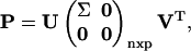(4)

where U ∈ ℛ^nxn is an orthonormal matrix of the left singular vectors (as columns in U), V ∈ ℛ^pxp is an analogous orthonormal matrix of the right singular vectors, and Σ ∈ ℛ^rxr is a diagonal matrix containing the singular values σ_i;

(5)

The diagonal elements of Σ are arranged in descending order such that σ₁ ≥ σ₂ ≥ … ≥ σ_r > 0. The first r columns of U and V, referred to as the left and right singular vectors, or modes, are unique and form the orthonormal basis for the column space and row space of P, respectively. The singular values are the square roots of the eigenvalues of P^TP (Lay, 1997). The magnitude of the singular values in Σ indicate the relative contribution of the singular vectors of U and V in reconstructing the P matrix. The second singular vector thus contributes less to the construction of P than the first singular vector, and its relative contribution can be assessed by the magnitude of its singular value compared to other singular values. All SVD calculations were performed using MATLAB (Mathworks, Natick, MA).

The fractional singular values were calculated by dividing each σ_i by the sum of all singular values. The cumulative fractional contribution is defined as the sum of the first n fractional singular values, where n can vary from 1 to r. Note that “singular vector” and “mode” are used interchangeably in this manuscript. The columns of U can be called “eigenpathways” and the rows of V^T can be called “eigenparticipations” (Fig. 2). The eigenparticipations (Fig. 2), or the modes of V, represent how the extreme pathways can be linearly combined to form the scaled modes of U, as illustrated in Eq. 6.

(6)

FIGURE 2.

The singular value decomposition of the extreme pathway matrix.

V gives the weightings on the pathways needed to reconstruct each of the modes of U as scaled by their respective singular values. P can be thought of as a matrix that operates upon a unit sphere, V, to form an ellipse that is elongated along each singular vector of U in proportion to the corresponding singular value in Σ (Lay, 1997). The modes referred to throughout this manuscript are the columns of U, or eigenpathways.

Extreme pathway decomposition

Each extreme pathway can be described as a weighted (positive or negative) linear combination of the first r modes of U, where r is the rank of P. Because the modes are orthonormal to each other, the weighting for each mode was found by taking the dot product of an extreme pathway with a given mode of U. The modal spectrum (or the set of r weightings) was calculated in this manner and gave insight into which mode is most important for constructing a particular extreme pathway.

CONCEPTUAL FRAMEWORK

Interpretation of the first mode

Computing the SVD of a convex basis for a solution space that lies within the positive orthant of the flux space ensures that the first mode must lie within the solution cone. In terms of the solution space of metabolic networks, this means that the first mode corresponds to a valid biochemical pathway through the network (i.e., mass balance and thermodynamic constraints are obeyed).

In general, the first mode, or first eigenpathway is directed down the middle of the space spanned by the extreme pathways (Fig. 3 A). In a symmetric cone, the first mode would come up through the geometric center of the cone (Fig. 3 B). However, if the cone is asymmetric, the first mode will be pulled more closely toward those portions of the cone with higher extreme pathway density. Portions of the extreme pathway cone that contain a high density of extreme pathways form “soft edges” and represent many systemically independent flux distributions that yield similar metabolic phenotypes. Thus, fluxes that are common in the extreme pathways will be reflected more heavily in the dominant mode of the cone. It should also be noted that the lengths of the extreme pathways can alter the direction of the first mode, where a longer extreme pathway will pull the first mode toward itself. In this study, however, all extreme pathways have unit length since the necessary v_max data is not available.

FIGURE 3.

Conceptual framework for application of singular value decomposition to extreme pathway analysis. In panel A, a convex representation of the cone defined by the extreme pathways is illustrated. The first mode from SVD analysis represents the principal direction of the cone. In panel B, the effect of symmetry of the convex cone is demonstrated. The areas shown represent cross sections of the multidimensional cone. The extreme pathways are represented by gray circles on the edges of the cone. The first mode is represented by a black circle inside the space. With “soft edges” in a cone, the dominant mode is “pulled” toward this region of the space. In panel C, we can see how the second and third principal modes characterize the convex cone. In the plane perpendicular to the first mode, the second and third modes characterize the variance in mutually perpendicular directions. Movement along the second mode allows for the most control of the space characterized by the first mode. In panel D, the effect of “soft edges” on the directions of the second and third mode is demonstrated.

Interpretation of subsequent modes

Each subsequent mode (or eigenpathway) after the first describes the direction of most variance in the subspace that is orthogonal to the previous modes. For example, the second mode describes the next direction in which most of the variance can be explained, and is orthogonal to the first mode. Fig. 3 C schematically demonstrates how the first three modes can characterize the solution space defined by the extreme pathways. Because each of the subsequent modes must be orthogonal to the first mode, they describe the cross section of the cone orthogonal to the dominant mode. Thus, in the three-dimensional case, the first mode defines the plane in which the second and third modes must lie. The second mode characterizes the direction that captures the most variance in this plane, and is the line with the minimum sum of squared differences between the line and all the extreme pathways. Thus, the direction of the mode is influenced by both the width of the cone in a particular direction and by the number of extreme pathways that are closely aligned along that direction. Thus, it can correspond to either the widest region of a cone (Fig. 3 C), or to a region that has a high extreme pathway density (Fig. 3 D). Because each of the modes is a linear combination of the extreme pathways, each mode satisfies the mass balance constraints. However, in contrast to the first mode, the subsequent modes individually will not necessarily satisfy reaction directionality constraints.

These subsequent modes represent important directions in the cone. For example, in Fig. 3 C, if extreme pathway 1 (EP₁) were the desired state, then the second principal mode could represent a critical regulatory modality. Movement of the solution from the flux distribution corresponding to the first mode to the desired state would be accomplished by moving in the direction defined by the second mode. Similarly, if extreme pathway 2 (EP₂) represented the desired state, then movement along the third principal mode would lead from the flux distribution corresponding to the first mode to the desired flux distribution. Moving a solution along a mode thus represents desired systemic regulatory control of the corresponding flux values.

Special case: subsets of orthogonal extreme pathways

Although the extreme pathways are not generally orthogonal to each other, it is possible in certain cases to have an extreme pathway or a subset of extreme pathways that are orthogonal to the rest. SVD of a cone containing extreme pathways that are orthogonal can generate modes that are identical to, or combinations of, these orthogonal pathways. Consequently, these components may not be represented in the first mode, inasmuch as they are decoupled from the rest of the extreme pathways. Although in general the first mode will involve the use of every flux used in any extreme pathway, it may not include fluxes that are only used in extreme pathways that are orthogonal to all other extreme pathways.

Interpretation of singular values

The singular values of the extreme pathway matrix characterize the amount of variance described by the directions of the corresponding modes. Large singular values indicate that a high degree of variance is captured in the direction of the corresponding mode. A large first fractional singular value means that the extreme pathways lie, on average, closer to the first mode in comparison to evenly distributed fractional singular values, which indicate that the extreme pathways are, on average, farther from the first mode.

SVD analysis of simple reaction networks

SVD of extreme pathway matrices of simple reaction networks demonstrated how important characterizations about the function of metabolic networks could be gained from this type of analysis. The system in Fig. 4 A is a simple linear chain of reactions. For this case, only one extreme pathway exists. The solution space is a degenerate cone; it is simply a line in the six-dimensional space characterized by the six fluxes. Thus, only one singular value exists and the first mode captures all of the variance of the one-dimensional solution space. This very simple case shows how a high first fractional singular value (in this case 1 or 100%) is a measure of how well the dominant mode represents the system. At 100%, the dominant mode represents the entire cone, because the cone is in fact this very line. Once one flux is set to a particular value, the values for all the other fluxes are fixed.

FIGURE 4.

Singular value decomposition of sample reaction networks. The SVD of these three reaction networks demonstrates how the SVD characterizes general properties of the solution cone, defining the phenotypic possibilities of the metabolic networks. In panel A, we have the simplest case—the linear chain of reactions has simply one extreme pathway, and consequently the first mode characterizes 100% of the extreme pathway matrix. This cone can be visualized as a simple vector, the “narrowest” possible case. In panel B, the system has four extreme pathways. Its first mode characterizes 47% of the total solution space. In panel C, the system has six extreme pathways. The first mode characterizes only 39% of the system. The first modes represent valid biochemical pathways in the network. The black and gray arrows in subsequent modes represent increased and decreased flux levels, respectively. The widths of all of the arrows in the representations of the modes are proportional to the flux through the corresponding reaction.

A slightly more complex example system demonstrates how the SVD describes flux variability allowed within the cone. The system in Fig. 4 B is defined by eight fluxes and four extreme pathways. However, the solution cone itself is a three-dimensional object, and thus there are three singular values. The first mode captures 47% of the variance. The second and third modes account for 28% and 22% of the variance, respectively. Because there are multiple modes, flexibility exists in the allowable ratios between the flux values.

Fig. 4 C shows a reaction network that is similar to the one in Fig. 4 B, but that contains one additional exchange flux. For the extreme pathway matrix of this system, there are four singular values, indicating a four-dimensional cone residing in the nine-dimensional flux space. The first, second, third, and fourth modes account for 39%, 22%, 20%, and 19% of the variance in the system, respectively. In Fig. 4 B, if the reaction that converts metabolite B to C is active, then the reaction that converts C to D is active, or the reaction that converts C to E is active, or both are active. However, this is not the case for the system in Fig. 4 C; there is the additional exchange flux for metabolite C. Thus, a wider range of steady-state solutions is available to the network.

The importance of the modes subsequent to the first is evident in Fig. 4, B and C. These subsequent modes illustrate important tradeoffs in the network where flux levels can be increased or decreased to change the steady-state flux distribution through the network. These tradeoffs in the metabolic network correspond to movement along the line described by the mode in the flux solution space. In the figure, the changes in the numerical value for fluxes shown in black are opposite to that of the fluxes shown in gray. Thus, if a black flux increases, a gray flux decreases, or vice versa. The second mode in panel B illustrates that for a given state of the network, if the reaction that converts C to D is increased, the reaction that converts C to E is decreased. This shift would move the solution point from a balanced D and E secretion (as seen in the first mode) to one that gives more weight to the secretion of D over E. In Fig. 4 B, the third mode illustrates a split at metabolite B. The exchange flux for metabolite A and the reaction that converts A to B are gray. The exchange flux for metabolite B and the fluxes for all subsequent processing reactions are black. The subsequent modes thus represent key branch points in the network and how they influence the flux distribution.

Similar tradeoffs can be seen in Fig. 4 C. In the second mode, the black fluxes involve the input of metabolite B, the conversion of B to C, and the output of C. All other fluxes are gray. If black is chosen to represent a flux increase with respect to the first mode, then B will be consumed and converted to C at a higher rate, whereas the consumption of A will decrease as well as the production of D and E. In the third mode, there is a split between the conversion of C to D or E (similar to that seen in the second mode of Fig. 4 B). In the fourth mode, one branch point is the production of C over the production of D and E.

Each of these subsequent modes obeys mass balance constraints, i.e., the magnitude of the increases in the fluxes out of a metabolite equals the magnitude of the fluxes that increase going into the metabolite. Consequently, in the second mode of Fig. 4 B and the third mode of Fig. 4 C, the black flux that leaves metabolite C has a value that is equal and opposite the gray flux that leaves metabolite C. This effect can also be seen in the fluxes around metabolite C in the fourth mode of Fig. 4 C. The black exchange flux leaving metabolite C is equal in magnitude to the sum of the black flux entering and the negative of the two gray fluxes leaving.

These sample systems illustrate how the SVD framework presented herein can elucidate systemic tradeoffs at key branch points in metabolic networks. Systemic tradeoffs represent critical decision points that affect what state the system can achieve and thus have relevance to regulation of the network. For instance, in the second mode of Fig. 4 B and the third mode of Fig. 4 C, metabolite C is a critical decision point where the output flux for D and the output flux for E can be changed.

RESULTS

SVD was applied to the extreme pathway matrices previously calculated for amino acid production in H. influenzae and H. pylori (Papin et al., 2002a; Price et al., 2002a). Briefly, the extreme pathway matrices were calculated for the synthesis of each of the nonessential amino acids of the two organisms. There are 17 nonessential amino acids in H. influenzae (alanine, asparagine, aspartic acid, glutamine, glycine, histidine, isoleucine, leucine, lysine, methionine, phenylalanine, proline, serine, threonine, tryptophan, tyrosine, and valine) and 12 in H. pylori (asparagine, aspartic acid, cysteine, glutamine, glutamatic acid, glycine, lysine, proline, serine, threonine, tryptophan, and tyrosine). Thus, a total of 29 extreme pathway matrices were studied. A list of the number of extreme pathways for each condition can be found in Fig. 5.

FIGURE 5.

Cumulative fractional contributions for the singular value decompositions of the extreme pathway matrices in H. influenzae and H. pylori. The cumulative fractional contribution is defined as the sum of the first n fractional singular values (reported as a percent). This value represents the contribution of the first n modes to the overall description of the system. The rank of the respective extreme pathway matrix is shown for nonessential amino acids. The S_crit value is the number of singular values that account for ≥95% of the variance in the matrices. Entries with “- - -” correspond to essential amino acids.

Singular values

The cumulative fractional contributions of the singular values (reported as a percent) are shown in Fig. 5. Each curve represents the cumulative fractional contribution of the modes to the extreme pathway matrix associated with a particular amino acid. For H. influenzae, the 17 curves (one for each nonessential amino acid) are shown in gray; For H. pylori, the 12 curves (one for each nonessential amino acid) are represented in black (see Fig. 5). The cumulative fractional contributions for the amino acids tightly cluster according to the respective organism. The difference between the average first fractional singular value and the average second fractional singular value in H. pylori is 0.20. The same difference in H. influenzae is 0.09. The effect of this difference can be seen in Fig. 5, where the cumulative fractional contribution increases faster for H. pylori than for H. influenzae. These results indicate a more even distribution of singular values in H. influenzae than in H. pylori.

Effective dimensionality

The rank of each of the extreme pathway matrices for amino acid production in H. pylori and H. influenzae was calculated. The number of singular values needed to characterize 95% of the variance (S_crit) was also evaluated (Fig. 5). The average rank for H. pylori extreme pathway matrices was 45, meaning that the convex space can be completely described by an average of 45 modes. However, 95% of the variance can be described by just the first 18 modes. Interestingly, even though H. influenzae had a smaller average rank (38) than H. pylori (45), more modes were needed in H. influenzae (between 22 and 24) than in H. pylori (18) to describe 95% of the variance. The effective dimensionality of the solution spaces (defined by a stringent 95% cutoff) was around one-half of the rank for both organisms.

Comparing dominant modes

Because the first mode best describes the variance of the entire cone, comparing the first modes of different extreme pathway matrices is a way to compare the direction of the two corresponding cones. The dominant modes of the extreme pathway matrices associated with the production of different amino acids were compared by calculating the angles between the modes for both H. pylori and H. influenzae. Dominant modes that lie in a similar direction (i.e., a small angle between modes) indicate that the principal utilization of the metabolic network is similar when achieving the different objectives. The angles between the first modes for the 17 amino acids in H. influenzae can be found in Table 1. The three smallest and the three largest pairs of angles were underlined and bold faced respectively. The three smallest pairs of angles were for tyrosine and phenylalanine (2.9°), asparagine and aspartic acid (3.8°), and serine and glycine (4.6°). The synthesis of tyrosine and phenylalanine differ by only a few final processing steps, explaining the proximity of their dominant modes. The three largest pairs of angles are for leucine and proline (25.1°), alanine and proline (22.4°), and leucine and threonine (22.1°). The angles between the second and third modes were also calculated, and the average angles are shown in Table 1. When analyzing the first, second, and third modes, alanine consistently had a high average angle in comparison to the other amino acids, which indicates that the convex solution cone for alanine production is the most distinct in the multidimensional space.

TABLE 1.

Angles between the first dominant modes of the extreme pathway matrices for amino acid synthesis in H. influenzae

	ALA	ASN	ASP	GLN	GLY	HIS	ILE	LEU	LYS	MET	PHE	PRO	SER	THR	TRP	TYR	VAL
ALA	0.0	–	–	–	–	–	–	–	–	–	–	–	–	–	–	–	–
ASN	14.9	0.0	–	–	–	–	–	–	–	–	–	–	–	–	–	–	–
ASP	14.6	3.8	0.0	–	–	–	–	–	–	–	–	–	–	–	–	–	–
GLN	16.8	7.9	9.0	0.0	–	–	–	–	–	–	–	–	–	–	–	–	–
GLY	16.6	6.0	7.1	8.1	0.0	–	–	–	–	–	–	–	–	–	–	–	–
HIS	17.6	9.0	10.9	11.5	11.2	0.0	–	–	–	–	–	–	–	–	–	–	–
ILE	15.0	11.2	10.4	14.2	13.7	16.0	0.0	–	–	–	–	–	–	–	–	–	–
LEU	18.8	19.2	19.8	20.4	19.5	19.2	19.7	0.0	–	–	–	–	–	–	–	–	–
LYS	13.3	9.6	9.0	12.6	12.4	14.2	7.9	18.6	0.0	–	–	–	–	–	–	–	–
MET	17.7	11.5	10.7	14.4	13.4	16.2	8.6	21.8	10.0	0.0	–	–	–	–	–	–	–
PHE	15.6	7.1	7.2	10.8	10.0	11.0	10.0	18.4	9.4	10.6	0.0	–	–	–	–	–	–
PRO	22.4	16.9	17.1	16.7	18.2	20.0	14.8	25.1	16.1	14.6	15.7	0.0	–	–	–	–	–
SER	15.3	4.7	5.6	7.9	4.6	10.2	12.0	18.8	10.7	11.9	8.2	17.1	0.0	–	–	–	–
THR	15.7	11.1	9.9	14.4	14.3	16.2	6.6	22.1	8.4	8.9	10.7	16.0	12.5	0.0	–	–	–
TRP	16.7	8.1	8.9	11.6	11.5	8.9	12.0	19.1	11.1	12.4	5.5	16.8	9.4	12.3	0.0	–	–
TYR	15.6	6.4	6.6	10.2	9.2	10.5	10.5	18.2	9.6	11.0	2.9	16.1	7.4	11.1	5.6	0.0	–
VAL	13.5	13.0	13.0	15.0	14.4	15.9	12.1	13.3	11.2	14.7	12.2	18.8	13.1	14.2	13.8	12.3	0.0
M1	16.3	10.0	10.2	12.6	11.9	13.7	12.2	19.5	11.5	13.0	10.3	17.6	10.6	12.8	11.5	10.2	13.8
M2	80.5	18.5	19.3	23.1	22.7	38.8	18.9	39.3	18.6	19.6	18.4	30.9	19.5	21.5	24.1	18.5	24.0
M3	76.7	35.5	35.0	40.8	39.2	47.8	52.1	49.2	56.0	48.9	34.9	56.3	35.8	61.8	39.0	35.0	62.6

The amino acids are represented by their three-letter abbreviation. The angles are in degrees. Also note that the matrix is symmetric, and consequently only half of the values are shown. The lowest angles between the first modes of the extreme pathway matrices for the production of the individual amino acids are underlined. The largest angles between the first modes are shown in boldface type. The row M1 corresponds to the average angle between the first mode of the extreme pathway matrix for the indicated amino acid and all of the other data sets. The row M2 corresponds to the average angle between the second modes. The row M3 corresponds to the average angle for the third mode.

Similar calculations were done for the set of extreme pathways for H. pylori amino acid synthesis (Table 2). The three smallest pairs for the first modes in the H. pylori extreme pathway matrices were serine and glycine (3.7°), glutamine and glutamatic acid (3.8°), and tyrosine and cysteine (3.9°). The three largest pairs were aspartic acid and proline (15.7°), asparagine and proline (14.9°), and glycine and proline (14.6°). The average angles between the first, second, and third modes are also indicated in Table 2.

TABLE 2.

Angles between the first dominant modes of the extreme pathway matrices for amino acid synthesis in H. pylori

	ASN	ASP	CYS	GLN	GLU	GLY	LYS	PRO	SER	THR	TRP	TYR
ASN	0.0	–	–	–	–	–	–	–	–	–	–	–
ASP	4.0	0.0	–	–	–	–	–	–	–	–	–	–
CYS	7.8	9.2	0.0	–	–	–	–	–	–	–	–	–
GLN	5.6	6.1	8.8	0.0	–	–	–	–	–	–	–	–
GLU	6.3	6.7	8.1	3.8	0.0	–	–	–	–	–	–	–
GLY	5.3	6.0	8.2	6.0	6.5	0.0	–	–	–	–	–	–
LYS	8.0	9.0	5.9	8.1	7.3	8.8	0.0	–	–	–	–	–
PRO	14.9	15.7	11.3	13.0	11.4	14.6	10.9	0.0	–	–	–	–
SER	4.7	5.7	6.5	5.3	5.6	3.7	7.2	13.3	0.0	–	–	–
THR	5.7	6.6	5.4	6.9	6.5	6.9	5.4	12.2	5.4	0.0	–	–
TRP	9.4	10.7	6.0	10.8	10.3	9.5	9.0	14.0	8.3	8.2	0.0	–
TYR	8.1	9.3	3.9	9.2	8.4	8.2	6.5	11.7	6.6	6.0	4.5	0.0
M1	7.2	8.1	7.4	7.6	7.4	7.6	7.8	13.0	6.6	6.8	9.2	7.5
M2	28.8	26.5	29.4	24.9	25.3	22.3	29.0	52.4	22.2	23.7	53.4	31.0
M3	33.7	35.7	40.8	33.1	31.7	32.1	35.5	64.2	29.8	30.8	48.0	36.8

The amino acids are represented by their three-letter abbreviation. The angles are in degrees. Also note that the matrix is symmetric and consequently only half of the values are shown. The lowest angles between the first modes of the extreme pathway matrices for the production of the individual amino acids are underlined. The largest angles between the first modes are shown in boldface type. The row M1 corresponds to the average angle between the first mode of the extreme pathway matrix for the indicated amino acid and all of the other data sets. The row M2 corresponds to the average angle between the second modes. The row M3 corresponds to the average angle for the third mode.

The relative proximity of the first modes tends to coincide with the biochemical precursors from which the individual amino acids are derived. The three largest angles between the first modes for the analyzed data sets in H. influenzae and H. pylori correspond to pairs of amino acids that are derived from different central metabolic precursors. For example, the largest angle in the H. influenzae data set is between the first modes corresponding to proline and leucine; proline is derived from α-ketoglutarate whereas leucine comes from pyruvate. In contrast, the three closest pairs in each case occur between amino acids that stem from the same precursor; the only exception is for cysteine and tyrosine in H. pylori. Examination of the first modes from these two extreme pathway sets shows that they both have higher fluxes through reactions involved in oxygen consumption, as compared to the first mode for tryptophan (which has a larger angle but is synthesized from the same precursor as tyrosine). This result indicates that the systemic production of cysteine and tyrosine consumes more oxygen then the systemic production of tryptophan in H. pylori. Thus, the angles between the first modes can be influenced by systemic considerations that are not evident based solely upon the identification of the key precursor in central metabolism.

Subsequent modes

The extreme pathways associated with histidine and alanine synthesis in H. influenzae were further analyzed to help identify possible control points in some of the subsequent modes. First, the extreme pathways that correspond to maximum histidine and alanine yield in H. influenzae were decomposed to ascertain the weightings for each of the modes that were necessary to reconstruct each pathway. There were 18 extreme pathways (out of 4934) with the maximum alanine yield and 64 extreme pathways (out of 4702) with the maximum histidine yield.

In Fig. 6, A and C, the extreme pathway decompositions are shown, with the weightings for each mode given on the y axis. Each line represents the modal spectrum for one extreme pathway. The modes with the maximum contribution to alanine or histidine production were determined by multiplying the mode's alanine or histidine exchange flux by the mode's weight.

FIGURE 6.

Key branch points in H. influenzae metabolic network for the synthesis of alanine and histidine. In panel A, there are 18 extreme pathways represented, each with the maximum yield of alanine. A key branch point in mode 2 of the metabolic network for alanine synthesis is shown in panel B. In panel C, there are 64 extreme pathways represented, each with the maximum histidine yield. A key branch point in mode 11 of the metabolic network for histidine synthesis is shown in panel D. Black and gray fluxes change in opposite directions. Dashed lines correspond to reactions not shown. Indicated metabolites are the following: E4P, erythrose 4-phosphate; F6P, fructose 6-phosphate; FDP, fructose-1,6-diphosphate; FRU, fructose; OA, oxaloacetate; PRPP, phosphoribosyl pyrophosphate; PYR, pyruvate; R5P, ribose 5-phosphate; RL5P, D-ribulose 5-phosphate; S7P, sedo-heptulose 7-phosphate; T3P1, glyceraldehyde 3-phosphate; T3P2, dihydroxyacetone phosphate; X5P, D-xylulose-5-phosphate. Reactions are catalyzed by the following enzymes: fba, fructose-1,6-bisphosphatate aldolase; fbp, fructose-1,6-bisphosphatase; pfkA, phosphofructokinase; prsA, phosphoribosyl pyrophosphate synthase; rpiA, ribose-5-phosphate isomerase A; talB, transaldolase B; tktA, transketolase; tpi, triosphophate isomerase.

For the alanine extreme pathway decomposition, mode 2 had the largest contribution to the net alanine production. This mode was inspected, and one branch point in the central metabolic network is indicated in Fig. 6 B. This branch point demonstrated an increase in the glycolytic flux that leads to the synthesis of pyruvate, a key precursor to alanine, and a decrease in the flux leading to the pentose phosphate reactions.

In the modal spectrum of the 64 extreme pathways with maximum histidine yield, mode 11 had the most significant contribution to a change in histidine flux. One branch point in this mode is indicated in Fig. 6 D. This branch point shifts flux from the pentose phosphate reactions (indicated in gray) to the reactions catalyzed by the rpiA and prsA gene products that lead to the synthesis of PRPP (phosphoribosyl pyrophosphate), a key precursor of histidine. Other branch points were present within the mode but are not shown.

DISCUSSION

This study presents the application of SVD to the analysis of large sets of extreme pathways generated from analysis of genome-scale metabolic networks. SVD of extreme pathway matrices has led to the following key results: 1), Convex steady-state solution cones characterizing the potential functions of biochemical networks were described using the modes generated by SVD, as readily illustrated by representative example systems; 2), SVD of extreme pathway matrices characterizing amino acid synthesis demonstrated that H. pylori has a more “rigid” metabolic network (lower effective dimensionality and more dominant first singular value). This interpretation is consistent with previously published results (Price et al., 2002a); and 3), SVD allowed for the comparison of different solution cones corresponding to the production of different amino acids within a genome-scale metabolic network.

Extreme pathways define a convex cone in a high-dimensional flux space that can be difficult to interpret and understand. The value of understanding the solution cone lies in its circumspection of all possible metabolic phenotypes available to a given network. SVD of extreme pathways gives several important measures that characterize these cones. First, the singular values can give a measure of the distribution of variance within the solution cone. A more even distribution of the contribution of the singular values is indicative of a cone that has wide variability with respect to its modes. Another important feature can be seen in the interpretation of the first mode; the first mode is a valid pathway through the network. With the exception of orthogonal extreme pathways (as was previously discussed), the first mode can be visualized as a single vector that characterizes the general direction of the cone. These features give very specific quantitative measures of the systemic capabilities of a network. It is important to note that SVD characterizes the linear, rather than the convex, space defined by the extreme pathways. Thus, the modes characterize a space that includes the complete solution space, but also span an additional space that is infeasible due to thermodynamic constraints. Therefore, not all combinations of the modes yield valid solutions. However, each valid flux distribution defined by the extreme pathways can be uniquely decomposed into the modes. It has been shown herein that it is possible to utilize SVD in such a manner that the decomposition yields insight to biological function.

This framework was subsequently applied to the analysis of the extreme pathway matrices for amino acid production in H. influenzae and H. pylori. The metabolic network for amino acid production in H. pylori was characterized by higher first fractional singular values and a lower effective dimensional space in comparison to the results from H. influenzae. These results are in agreement with previously published analyses that demonstrated a much more restricted metabolic potential for H. pylori than H. influenzae (Papin et al., 2002a; Price et al., 2002a). Understanding and characterizing the metabolic potential of pathogens like H. pylori and H. influenzae can also lead to the targeting of an organism's weaknesses, important for therapeutic purposes and metabolic engineering design.

The comparison of solution cones can be challenging because cones differ in their dimensionality. Direct comparisons can only be made for cones of the same dimension and with the same fluxes. SVD can be used to facilitate rough comparisons between cones. The first mode describes the direction of most variance within the cone. Thus, by comparing the angle between the first mode of different cones, a comparison can be made between the general directions of the two cones. The first modes must contain the same sets of fluxes to be compared directly. For this reason, the comparisons made between the first modes of solution cones were only made within the same organism and for the production of one amino acid with all other allowable fluxes being identical (i.e., the same stoichiometric matrix). Thus, for these calculations we were able to make comparisons between solution cones.

Subsequent modes may serve to further the understanding of regulatory logic in metabolic networks. The subsequent modes of the SVD characterize orthogonal pathways that describe the variance in the flux space. An interpretation of these modes will enable the characterization of the tradeoffs in flux values that best reconstruct the solution space. The subsequent modes identify key branch points in the network, which are potential control points for regulation. Thus, these subsequent modes can be thought of as finding key regulatory modalities. They represent orthogonal directions in the space, and thus they are uncoupled from each other in a mathematical sense. However, biological systems are not constrained by the need for orthogonal regulatory modalities. Once the subsequent modes that best represent the solution space (or a portion of the solution space that is of most interest) are calculated, these modes can be transformed into nonorthogonal, biologically meaningful vectors. A need exists for the elucidation of optimal criteria for decoupling these predicted regulatory modalities based upon biochemical considerations, rather than by the mathematical definition of orthogonality. The elucidation of the way in which the subsequent modes describe cellular regulation warrants further study, as does an investigation of the criteria by which these subsequent modes can be transformed to maximize insight into the regulation of biological systems.

Extreme pathways are becoming an important tool for the analysis of metabolic networks. Flux balance analysis (Edwards et al., 1999), kinetic theory (Reich and Sel'kov, 1981; Heinrich and Schuster, 1996), elementary modes (Schuster et al., 2000), and metabolic control analysis (Fell, 1996) have yielded biologically important results. Extreme pathway analysis generates a unique and minimal set of basis vectors that circumscribe all possible steady-state flux solutions of a metabolic network. As such, the understanding and analysis of extreme pathways result in time-invariant, systemic characterizations of the full capabilities of an organism. SVD of extreme pathway matrices is a novel application for reducing the dimensionality of these data sets and providing succinct characterizations of the metabolic solution space.

Taken together, the SVD of extreme pathway matrices has led to interesting and important characterizations of the properties of metabolic networks, and may potentially provide clues to inherent systemic regulatory structures. The results presented herein point to how emergent properties can be elucidated from systemic in silico analyses. As the amount of genomic data expands, approaches such as extreme pathway analysis and the SVD of its resultant pathways will lead to a systemic understanding of biological systems.

References

- Alter, O., P. O. Brown, and D. Botstein. 2000. Singular value decomposition for genome-wide expression data processing and modeling. Proc. Natl. Acad. Sci. U.S.A. 97:10101–10106. [DOI] [PMC free article] [PubMed] [Google Scholar]
- Beard, D. A., S. Liang, and H. Qian. 2002. Energy balance analysis for complex metabolic networks. Biophys. J. 83:79–86. [DOI] [PMC free article] [PubMed] [Google Scholar]
- Bonarius, H. P. J., G. Schmid, and J. Tramper. 1997. Flux analysis of underdetermined metabolic networks: the quest for the missing constraints. Trends Biotechnol. 15:308–314. [Google Scholar]
- Carlson, R., D. Fell, and F. Srienc. 2002. Metabolic pathway analysis of a recombinant yeast for rational strain development. Biotechnol. Bioeng. 79:121–134. [DOI] [PubMed] [Google Scholar]
- Covert, M. W., C. H. Schilling, I. Famili, J. S. Edwards, I. I. Goryanin, E. Selkov, and B. O. Palsson. 2001. Metabolic modeling of microbial strains in silico. Trends Biochem. Sci. 26:179–186. [DOI] [PubMed] [Google Scholar]
- Drell, D. 2002. The Department of Energy microbial cell project: A 180 degrees paradigm shift for biology. OMICS. 6:3–9. [DOI] [PubMed] [Google Scholar]
- Edwards, J. S., and B. O. Palsson. 1999. Systems properties of the Haemophilus influenzae Rd metabolic genotype. J. Biol. Chem. 274:17410–17416. [DOI] [PubMed] [Google Scholar]
- Edwards, J. S., R. Ramakrishna, C. H. Schilling, and B. O. Palsson. 1999. Metabolic flux balance analysis. In Metabolic Engineering. S. Y. Lee and E. T. Papoutsakis, editors. Marcel Dekker, New York. 13–57.
- Fell, D. A. 1996. Understanding the Control of Metabolism. Portland Press, London
- Heinrich, R., and S. Schuster. 1996. The Regulation of Cellular Systems. Chapman and Hall, New York
- Lay, D. C. 1997. Linear Algebra and Its Applications. Addison Wesley Longman, Boston
- Liao, J. C., S. Y. Hou, and Y. P. Chao. 1996. Pathway analysis, engineering and physiological considerations for redirecting central metabolism. Biotechnol. Bioeng. 52:129–140. [DOI] [PubMed] [Google Scholar]
- Papin, J. A., N. D. Price, J. S. Edwards, and B. O. Palsson. 2002a. The genome-scale metabolic extreme pathway structure in haemophilus influenzae shows significant network redundancy. J. Theor. Biol. 215:67–82. [DOI] [PubMed] [Google Scholar]
- Papin, J. A., N. D. Price, and B. O. Palsson. 2002b. Extreme pathway lengths and reaction participation in genome-scale metabolic networks. Genome Res. 12:1889–1900. [DOI] [PMC free article] [PubMed] [Google Scholar]
- Price, N. D., J. A. Papin, and B. O. Palsson. 2002a. Determination of redundancy and systems properties of helicobacter pylori's metabolic network using genome-scale extreme pathway analysis. Genome Res. 12:760–769. [DOI] [PMC free article] [PubMed] [Google Scholar]
- Price, N. D., I. Famili, D. A. Beard, and B. O. Palsson. 2002b. Extreme pathways and Kirchhoff's second law (letter to the editor). Biophys. J. 83:2879–2882. [DOI] [PMC free article] [PubMed]
- Reich, J. G., and E. E. Sel'kov. 1981. Energy Metabolism of the Cell: A Theoretical Treatise. Academic Press, New York
- Samatova, N. F., A. Geist, G. Ostrouchov, and A. V. Melechko. 2002. Parallel out-of-core algorithm for genome-scale enumeration of metabolic systematic pathways. Proceedings of the First IEEE Workshop on High Performance Computational Biology (HiCOMB 2002). Ft. Lauderdale, Florida. p. 185.
- Schilling, C. H., and B. O. Palsson. 2000. Assessment of the metabolic capabilities of Haemophilus influenzae Rd through a genome-scale pathway analysis. J. Theor. Biol. 203:249–283. [DOI] [PubMed] [Google Scholar]
- Schilling, C. H., D. Letscher, and B. O. Palsson. 2000. Theory for the systemic definition of metabolic pathways and their use in interpreting metabolic function from a pathway-oriented perspective. J. Theor. Biol. 203:229–248. [DOI] [PubMed] [Google Scholar]
- Schilling, C. H., M. W. Covert, I. Famili, G. M. Church, J. S. Edwards, and B. O. Palsson. 2002. Genome-scale metabolic model of Helicobacter pylori 26695. J. Bacteriol. 184:4582–4593. [DOI] [PMC free article] [PubMed] [Google Scholar]
- Schuster, S., D. A. Fell, and T. Dandekar. 2000. A general definition of metabolic pathways useful for systematic organization and analysis of complex metabolic networks. Nat. Biotechnol. 18:326–332. [DOI] [PubMed] [Google Scholar]
- Varma, A., and B. O. Palsson. 2002. Metabolic flux balancing: basic concepts, scientific and practical use. Bio-Technol. 12:994–998. [Google Scholar]
- Wiback, S. J., and B. O. Palsson. 2002. Extreme pathway analysis of human red blood cell metabolism. Biophys. J. 83:808–818. [DOI] [PMC free article] [PubMed] [Google Scholar]
- Yeung, M. K., J. Tegner, and J. J. Collins. 2002. Reverse engineering gene networks using singular value decomposition and robust regression. Proc. Natl. Acad. Sci. USA. 99:6163–6168. [DOI] [PMC free article] [PubMed] [Google Scholar]