Mechanical Coupling via the Membrane Fusion SNARE Protein Syntaxin 1A: A Molecular Dynamics Study

Abstract

SNARE trans complexes between membranes likely promote membrane fusion. For the t-SNARE syntaxin 1A involved in synaptic transmission, the secondary structure and bending stiffness of the five-residue juxtamembrane linker is assumed to determine the required mechanical energy transfer from the cytosolic core complex to the membrane. These properties have here been studied by molecular dynamics and annealing simulations for the wild-type and a C-terminal-prolongated mutant within a neutral and an acidic bilayer, suggesting linker stiffnesses above 1.7 but below 50 × 10⁻³ kcal mol⁻¹ deg⁻². The transmembrane helix was found to be tilted by 15° and tightly anchored within the membrane with a stiffness of 4–5 kcal mol⁻¹ Å⁻². The linker turned out to be marginally helical and strongly influenced by its lipid environment. Charged lipids increased the helicity and H3 helix tilt stiffness. For the wild type, the linker was seen embedded deeply within the polar region of the bilayer, whereas the prolongation shifted the linker outward. This reduced its helicity and increased its average tilt, thereby presumably reducing fusion efficiency. Our results suggest that partially unstructured linkers provide considerable mechanical coupling; the energy transduced cooperatively by the linkers in a native fusion event is thus estimated to be 3–8 kcal/mol, implying a two-to-five orders of magnitude fusion rate increase.

INTRODUCTION

For exocytosis and for the selective transport of macromolecules between the various organelles of eukaryotic cells, the fusion of a transport vesicle membrane with a target membrane is an essential step (Alberts et al., 2002). A complex network of sequentially interacting proteins is involved in the tethering and docking of the vesicles, as well as the promotion and regulation of the fusion process (Misura et al., 2000; Mochida, 2000). For synaptic transmission, the highly conserved SNARE (soluble N-ethylmaleimide sensitive factor attachment protein receptor) proteins (Söllner et al., 1993) have been identified as central players and studied in detail (Hanson et al., 1997; Jahn and Südhof, 1999; Chen and Scheller, 2001), and specific sets of SNARE homologs were also found for a number of other transport pathways (Bennett and Scheller, 1993; Ferro-Novick and Jahn, 1994). Although the precise role of SNARE proteins in membrane fusion is still a subject of ongoing discussions (Ungermann et al., 1998; Tahara et al., 1998; Mayer, 1999; Brünger, 2001; Bruns and Jahn, 2002; Jahn and Grubmüller, 2002), in vitro fusion experiments suggest that SNAREs form a minimal fusion machinery (Weber et al., 1998; Nickel et al., 1999). According to the zipper model of membrane fusion (Hay and Scheller, 1997; Hanson et al., 1997; Bruns and Jahn, 2002), vesicle (v) and target (t) membrane-anchored SNAREs assemble in a zipperlike fashion into extended trans complexes (see Fig. 1). Because both ends are anchored within the membranes via transmembrane (TM) domains (tilted yellow and magenta rectangles), the membranes are pulled into close proximity, thus promoting fusion.

FIGURE 1.

Model for SNARE-promoted membrane fusion. A trans complex is formed by synaptobrevin and SNAP-25 (blue), the H3 helix of syntaxin (cyan), a linker region (red), the transmembrane (TM) domains (tilted rectangles) of syntaxin (yellow), and synaptobrevin (magenta), which exerts mechanical force onto the vesicle (v) and the target (t) membrane and pulls them toward each other. The H3 helix tilt θ (pink) is studied in molecular dynamics simulations; the brown box marks the simulation system. The hydrophobic regions of the two membranes are colored green, their polar regions dark green.

Consistent with this model is the structure of the cytosolic core of the SNARE complex, which has been resolved by x-ray crystallography (Sutton et al., 1998). It forms a four-stranded parallel coiled-coil, to which one helix (H3, cyan) is contributed by the t-SNARE syntaxin 1A, a second by the v-SNARE synaptobrevin-II (magenta), and two more by the t-SNARE SNAP-25 (blue). The hydrophobic TM domains of synaptobrevin and syntaxin have been predicted to consist of 19 (95–113) and 22 (266–287) residues, respectively, which is sufficient to form bilayer-spanning α-helices perpendicular to the membrane plane (Sutton et al., 1998). Further support for the α-helical structure of the TM domains is obtained from several studies (Laage and Langosch, 1997; Laage et al., 2000; Langosch et al., 2001). It has been proposed (McNew et al., 2000) that pulling on the membrane anchor displaces it from the bilayer, dragging out associated lipids toward the contact area between the two bilayers, and thus triggers membrane fusion.

It has been suggested (Weber et al., 1998) that formation of the trans complex induces significant strain within the membrane-proximate regions of synaptobrevin (magenta) and syntaxin (red, linker), respectively. Thus, and assuming that the TM helices remain perpendicular to the local membrane plane, energy provided by complex formation could, via a conformational coupling, be transmitted to the bilayers and thereby induce membrane bending as shown in Fig. 1. Evidently, the coupling efficiency critically depends on the mechanical bending stiffness of the membrane-proximate regions. In particular, the energy available for membrane juxtaposition is limited by the amount required to increase the H3 helix tilt angle θ (pink) from its equilibrium value to the one required for SNARE complex assembly.

For synaptobrevin, the α-helical domain of the synaptic fusion complex x-ray structure (core domain) extends into the TM domain by two residues; this suggests that core and TM domain form a continuous α-helix, which is expected to be stiff upon bending (Shaitan et al., 2002). Membrane bending and final merger allowed the synaptobrevin helix to gradually relax to an unbent state (McNew et al., 1999).

For syntaxin, the H3 helix is separated from the TM helix by a five-residue basic linker (red) of unknown structure. The only information comes from recent electron paramagnetic resonance (EPR) measurements, which provided some evidence for an unstructured linker (Kweon et al., 2002). Hence it is unclear if a similar mechanism holds here. In fact, inserting the five-residue sequence GPPKL containing two helix-breaking proline residues into the linker of syntaxin reduced the in vitro fusion rate by only 50% (McNew et al., 1999). Similarly, for a syntaxin homolog in yeast, a six-residue insertion between the expected core and the TM domain led to a comparable fusion rate decrease in vivo. The effect of the proline insertions on the linker stiffness is, however, unclear. Although disfavoring α-helical conformations, it can also rigidify the protein backbone (Schultz and Schirmer, 1979). Moreover, a similar proline mutation of synaptobrevin had virtually no effect on fusion efficiency (McNew et al., 1999). These results suggest that either a stiff linker is not required for fusion, or sufficient conformational coupling can also be provided by a nonhelical linker.

To discriminate between these two possibilities, we have performed multinanosecond molecular dynamics (MD) simulations of the relevant region (Fig. 1, box; see also Fig. 6) comprising a 39-residue C-terminal part of syntaxin (cyan, red, and yellow) embedded within a lipid bilayer (green) and explicit solvent environment (in Fig. 6 water molecules are shown in blue). In particular, the following questions were addressed: 1), What is the native structure of the five-residue syntaxin linker? Is it α-helical? 2), Can a nonhelical linker also provide substantial conformational coupling? 3), Can the bending stiffness be estimated from the simulations? 4), Which factors (e.g., lipid composition, environment, sequence) determine the mechanical properties of the linker? 5), Is the TM domain sufficiently perpendicular to the membrane plane, as required for conformational coupling? 6), Is the TM domain anchored well enough within the membrane to withstand the high intermembrane repulsion forces due to hydration and electrostatic interactions (Lipowsky, 1995), which tend to pull the TM domain out of the membranes?

FIGURE 6.

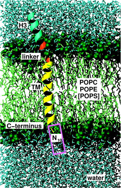
Simulation system setup. Shown is the C-terminal segment of syntaxin, comprising an 11-residue segment of the H3 helix (Asp-250–Lys-260, cyan), the five-residue basic linker (Ala-261–Lys-265, red), and the 23-residue TM helix (Ile-266–Gly-288), embedded in a lipid bilayer (green, the green spheres indicate the phosphor, oxygen, and nitrogen atoms of the polar regions), with an explicit solvent environment (water molecules are shown in blue; ions are not shown). The magenta rectangle indicates the position of the 10-asparagine prolongation present in some of the simulations.

These questions were addressed by analyzing the equilibrium distributions of appropriate reaction coordinates as obtained from room-temperature simulations (first part), and, to improve the sampling, from sets of simulated annealing end structures (second part).

METHODS

Room-temperature and annealing simulations were carried out for various systems. From these simulations, free-energy landscapes for relevant observables, such as helix tilts and vertical peptide position within the membrane, were obtained.

Room temperature simulations

Simulation systems

MD simulations were carried out for three peptides (compare Table 1): the wild-type (WT), a WT peptide with a truncated TM domain (WT^S), and mutant prolonged by 10 asparagine residues (N₁₀) described below.

TABLE 1.

Simulated peptides

Peptide	Nr	Residues	q[e]	Na
WTS	22	253–274	+7	234
WT	39	250–288	+6	373
N10	49	WT + Asn10	+6	483

A wild-type peptide with a full TM domain (WT) and one with a with a truncated TM domain (WT^S), as well as a prolonged mutant (N₁₀), were simulated. Given are the respective number of residues (N_r), the net charge (q), and the number of atoms (N_a).

Each peptide comprised the syntaxin 1A linker, the TM domain, and cytosolic residues of the H3 helix, and was embedded in an explicit lipid and solvent environment. Fig. 6 shows, as an example, the WT with the TM domain (Ile-266–Gly-288, yellow), the five-residue linker (Ala-261–Lys-265, red), and the cytosolic H3 helix (Asp-250–Lys-260, cyan) embedded within a lipid bilayer (green). The magenta rectangle indicates the position of the N₁₀ prolongation. The N-termini of the peptides are artificial termini and were therefore modeled neutral (i.e., as NH₂). The C-termini were modeled charged (i.e., as COO⁻). To include the stabilizing effect of the coiled-coil helices that were present in the crystal structure but not included within the simulation system, the secondary structure of the H3 helix was stabilized by internal restraints as described below.

Table 2 specifies the two lipid compositions that were chosen to study the influence of the lipid environment on the peptide properties. A neutral bilayer (POP⁰) was created with a binary lipid mixture of zwitterionic palmitoyl-oleoyl-phosphatidylcholine (POPC) and palmitoyl-oleoyl-phosphatidylethanolamine (POPE) molecules, and a more physiological acidic bilayer (POP-) with a ternary lipid mixture of POPC, POPE, and palmitoyl-oleoyl-phosphatidylserine (POPS) molecules. Table 3 summarizes all simulated systems that fall into three sets. Set A contains the four possible combinations of the peptides WT and N₁₀ with bilayers POP⁰ and POP⁻ and was used for the main production runs at T = 300 K. Set B was used for additional annealing runs. Set C was used to obtain first insight into membrane effects, e.g., by simulating a simple van der Waals membrane (VdW, see below). The WT systems comprised ∼20, 000 atoms, including 373 peptide atoms, and the N₁₀ systems comprised ∼22, 000 atoms, including 483 peptide atoms. All simulation systems with explicit lipid environment were set up in rectangular boxes with periodic boundary conditions and lateral dimensions a × b of ∼60 Å × 60 Å. The box sizes in the z direction (84–88 Å) were chosen such as to obtain a minimum distance of 7 Å between the peptide-membrane system and the boundary in z direction, yielding a water layer of ∼30 Å between the membranes.

TABLE 2.

Simulated bilayers

Bilayer	POPC	POPE	POPS	q[e]	Na
POP0	70	46	–	0	6032
POP−	70	34	12	−12	6068

A neutral (POP⁰) and an acidic bilayer (POP⁻) were simulated containing the zwitterionic lipids POPC and POPE, and the acidic lipid POPS. The net charge of the bilayer is denoted by q, and the number of lipid atoms by N_a.

TABLE 3.

Simulation systems

Set	Simulation system	Peptide	Bilayer	Nw	Ions	Na	a × b × c [Å3]
A	WT/POP0	WT	POP0	4718	6 Cl−	20565	56.9 × 61.8 × 88.0
	WT/POP−	WT	POP−	4725	6 Na+	20622	56.5 × 61.3 × 84.2
	N10/POP0	N10	POP0	5292	6 Cl−	22397	60.0 × 61.8 × 88.0
	N10/POP−	N10	POP−	5046	6 Na+	21695	57.0 × 61.8 × 88.0
B	WT/POP−/SALT	WT	POP−	4697	17 K+, 11 Cl−	20560	56.5 × 61.3 × 84.2
	WTH/POP0	WT	POP0	4055	6 Cl−	18576	65.8 × 71.4 × 107.1
C	WTS/–	WTS	–	3036	7 Cl−	9353	51.3 × 51.3 × 51.3*
	WTS/VdW	WTS	VdW	4874	7 Cl−	14863	59.9 × 59.9 × 59.9*

Peptides are specified in Table 1, bilayers in Table 2. Given are the respective number of water molecules (N_W), the number of atoms (N_a), and the initial box size (a × b × c).

^*Dodecahedron box with angles 60°, 60°, and 90°.

Restraints

In the simulations, several restraints were imposed on peptide, lipid, and water molecules. For position restraints, the position restraint potential of GROMACS (Van der Spoel et al., 1995) with the initial coordinates as reference positions, and a force coefficient (just small enough for the respective vibration period to exceed the chosen integration stepwidth by at least a factor of eight) 358 kcal mol⁻¹ Å⁻² was used. Selected helical peptide segments were stabilized on the backbone O_i-N_i+3 atom pairs by imposing the distance restraint potential implemented in GROMACS (Van der Spoel et al., 1995), which was chosen constant for distances smaller than 3 Å, harmonic between 2 and 6 Å with force constant 239 kcal mol⁻¹ Å⁻², and linear for larger distances (1–4 distance restraints). For the elevated temperature runs of the annealing simulations, additional restraints (backbone dihedral restraints) were imposed on all backbone dihedral angles φ, ψ, and ω of the H3 and the TM helices (and of the prosequence, if present), and the ω angles of the linker, by defining supplementary dihedrals (Van der Spoel et al., 1995) for the peptide, with φ₀ = α + 180°, α denoting the initial value of the dihedral, and a force constant of k_φ = 191 kcal mol⁻¹deg⁻².

Solvation methods

Systems were solvated by filling the periodic box with water molecules and removing all those water molecules that overlapped with the peptide or lipid atoms. For the explicit lipid bilayer, also all water molecules within the hydrophobic core of the bilayer were removed. Ions were added by replacing water molecules at energetically favorable positions (Coulomb criterion), or in shells of radius 10 Å around oppositely charged groups (Debye criterion). If not denoted otherwise, the type (Cl⁻ or Na⁺) and number of ions were chosen so as to compensate the net charge of the peptide-membrane system (charge compensation). In one case, excess ions were added and K⁺ rather than Na⁺ ions were used to mimic the intracellular conditions of typical mammalian cells (Alberts et al., 2002), and, in particular, to obtain a physiological concentration of [KCl] = 0.154 M, (intracellular salt conditions).

Pilot studies: absent and simplified lipid environment

To check whether the lipid environment is relevant for the linker structure and, therefore, should be included within the production simulations, two simulations of 2 ns length each without explicit lipid environment were carried out (Table 3, Set C). The first simulation involved no lipid bilayer at all, the second a simplified bilayer model. Accordingly, a peptide with a truncated WT^S could be used. The conformations of two linker residues (Ala-261 and Arg-262) obtained from these simulations were used to model a linker start structure that was improved in subsequent simulations with explicit lipid environment.

Fig. 2 helps the reader to keep track of the various simulations and their interdependencies both for the pilot runs as well as, in particular, for the subsequent equilibrium and annealing runs. To obtain a start structure (see Fig. 3, top left), Protein Data Bank (PDB) data (where available), and modeling were combined (see Fig. 2, green boxes). The H3 helix was taken from chain F of the x-ray structure (Sutton et al., 1998), PDB entry 1sfc (green arrows from PDB box). The TM domain was modeled as a right-handed α-helix using Insight II (Molecular Simulations, Cambridge, UK). The linker was modeled with its dihedral angles chosen from the β-region of the Ramachandran plot (Ramachandran et al., 1963) (for the side-chain dihedrals, the default settings of Insight II were used). Because in the pilot study the peptide was truncated at both ends, both termini were modeled neutral (NH₂ and COOH, respectively). Both modeling procedures are summarized by the respective green box and arrows.

FIGURE 2.

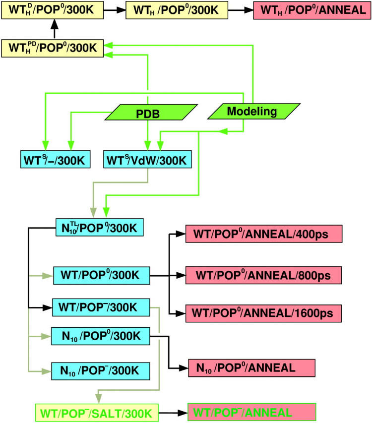
Overview of simulation runs and their mutual interdependencies. Blue (or yellow) and red boxes denote room-temperature runs at T = 300 K (also tagged 300K), and annealing sets (ANNEAL), respectively; green fonts indicate simulations with intracellular salt conditions. Green arrows denote input from the Protein Data Bank or major modeling steps; black and gray arrows indicate that a final configuration has been used as a starting configuration for a subsequent simulation, either without (black) or with (gray) modification. For nomenclature and specification of the various simulation systems, see Table 3.

FIGURE 3.

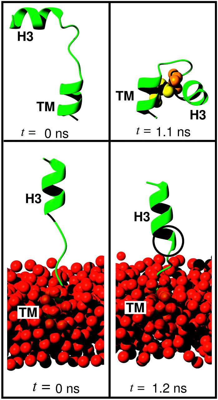
Starting peptide structures (left) and intermediate structures (right) of the two pilot simulations described in the text, without lipid environment (top), and with simplified lipid environment (bottom). In the top right figure, the spheres show the residue pair forming a hydrophobic contact, which stabilized the final structure of the peptide, i.e., the linker residue Ala-261 (orange) and the TM residue Ile-270 (yellow). In the bottom panel, the position-restrained water oxygen atoms that mimic the sterical effect of a bilayer are shown as red spheres. In the bottom right figure, the black circle marks the two linker residues that spontaneously folded from loop into α-helical conformation.

For the WT^S/–/300 K simulation without lipid environment (blue box, left column), periodic boundary conditions with a dodecahedron box were used. The box dimensions were chosen so as to obtain a minimum distance of 7 Å between the centered peptide and the boundary. After solvation, 7 Cl⁻ ions were inserted for charge compensation according to the Coulomb criterion. To mimic the helix-stabilizing effect of the membrane, the TM helix was subjected to 1–4 distance restraints.

The system WT^S/VdW (Fig. 3, bottom left) was set up in a similar manner. To mimic the reduced conformational space available for the peptide due to the presence of the lipid bilayer, the oxygen atoms of all water molecules in a 5-Å layer perpendicular to the TM helix (red spheres) were subjected to position restraints. Additionally, position restraints were imposed onto the backbone atoms of the TM helix. The linker conformation was changed such that the side chains of the linker and the H3 helix did not penetrate the membrane layer.

Production runs: explicit solvated lipid environment

In the simulation, WT^S/VdW/300 K, after 0.3 ns, two residues of the linker, namely Ala-261 and Arg-262, adopted an α-helical conformation (Fig. 3, bottom right, black circle), which remained stable for 0.9 ns. Therefore the linker structure after 1.2 ns was taken as the start structure of the first simulation with explicit lipid environment, (Fig. 2, gray arrow).

The start structures of the H3 and the TM helix were obtained similarly as for WT^S, except that three more H3 residues and the full TM domain (including Gly-288) were included. The TM helix was modeled using MOLMOL (Koradi et al., 1996); the side-chain dihedrals were set to the default values provided by MOLMOL.

For the lipid environment, an equilibrated bilayer of 128 POPC molecules kindly provided by P. Tieleman (Tieleman, 1998, 2000) was used. For the peptide insertion, a cylindrical hole of radius 7 Å was created by removing those four lipid molecules from each layer, whose headgroups were located within the hole region. Subsequently, a weak repulsive and radially acting force centered at the vacated region was applied to the lipid molecules during a short MD run to remove lipid tail atoms from the hole region (Tieleman, 1998).

As can be seen in Fig. 6, severe steric conflicts between the linker of the peptide (red) and several lipid headgroups (green), which could not be resolved by minor changes of the backbone configuration of the three remaining nonhelical residues, prohibited complete peptide insertion. As a result, the TM helix protruded at its N-terminal side into the polar region of the bilayer by ∼5 Å, whereas, at the C-terminus, a hole within the hydrophobic core of the bilayer of about the same length remained. To avoid closure of that hole, a prosequence of 10 α-helical asparagine residues, modeled in α-helical conformation, was appended at the C-terminus (N₁₀ mutant) with the expectation that the peptide would relax and shift downward during the equilibration phase to fully bury the apolar TM residues in the hydrophobic core of the bilayer, such that the prosequence could then be removed. For the prosequence, the choice of asparagines was motivated by the expectation that their high polarity (Stryer, 1988) should drive them quickly out of the hydrophobic region of the bilayer. Furthermore, the neutral asparagines should disturb the system only slightly.

Two POPC molecules of each layer still overlapped with the peptide and were removed. To obtain the desired lipid composition of the neutral bilayer, 46 uniformly distributed lipid molecules were mutated into POPE molecules. The system was then solvated and subsequently equilibrated for 5 ns the superscripts denote 1–4 distance restraints for the TM helix (T) and two linker residues Ala-261 and Arg-262 (L).

From the final structure of this trajectory, the set of the four possible combinations of lipid environment and peptide type (Table 3, Set A) was obtained as shown in Fig. 2 as follows: The system N₁₀/POP⁰ was transformed into WT/POP⁰ by removing the prosequence, modeling a new C-terminus, and filling the resulting cavity with water molecules. The two POP⁰ systems (WT/POP⁰ and N₁₀/POP⁰) were transformed into respective POP⁻ systems by removing the solvent environment, mutating selected POPE into POPS molecules, resolvating the system, and adding ions for charge compensation according to the Debye criterion. For each of the four obtained systems, free dynamics production runs of 5 ns length each were carried out (four blue boxes) for further analysis and computation of free-energy landscapes. Two final structures (taken from WT/POP⁰/300 K and N₁₀/POP⁰/300K) served as starting structures for subsequent high temperature runs (red boxes).

Further room-temperature simulations were performed as shown in Fig. 2 (Table 3, Set B). From the equilibrated system WT/POP⁻, a system with intracellular salt conditions was created by changing the Na⁺ into K⁺ ions and inserting excess K⁺ and Cl⁻ ions according to the Coulomb criterion. To check for a possible bias of the chosen linker start structure, an independent line of simulations was performed. These started with simulation (second box, left column) with the linker now modeled in fully α-helical conformation (subscript H). Here, no steric hindrance occurred in the polar region, and the peptide could be readily inserted, so no membrane-stabilizing prosequence had to be appended. Otherwise, the simulation system was set up similar to To equilibrate the lipid environment, the peptide was first immobilized by position restraints on the backbone atoms of the TM domain (superscript P) and, in addition to helix H3 and the TM domain, also the linker was subjected to 1–4 distance restraints (D). In subsequent simulations, position and distance restraints (WT_H/POP⁰/300 K) were successively removed.

Simulation parameters

All simulations were performed with the GROMACS simulation package (Van der Spoel et al., 1995), version 2.1, using the GROMOS-87 force field (van Gunsteren and Berendsen, 1987) with modifications (van Buuren et al., 1993). Polar hydrogen atoms were simulated explicitly; nonpolar hydrogen atoms were described via compound atoms. The SPC water model (Hermans et al., 1984) was used. The POPC force field originated from Berger et al. (1997), parameters for the unsaturated carbons and POPE parameters from the GROMOS-87 force field; the POPS force field (Knecht, Ph.D., thesis, University Göttingen (unpublished)) was derived from the POPE parameters using serine as a template. Using LINCS (Hess et al., 1997) to constrain the bond lengths, and heavy hydrogen atoms (Feenstra et al., 1999), a time step of 4 fs could be chosen. For the trajectories of the pilot study, light hydrogen atoms and a time step of 2 fs were used.

To calculate the nonbonded forces, a twin-range cutoff was used on a charge group basis: In each step, short-range electrostatic and van der Waals forces were calculated for all pairs of a neighbor list with nearest-image distances r ≤ r_list = 10 Å; the neighbor list, as well as the long-range electrostatic force on each particle due to all particles in a shell r_list < r ≤ 18 Å, were updated every 10 steps (in the pilot studies, this was done for a shell r_list < r ≤ 15 Å). For the intracellular salt condition simulations, the particle mesh Ewald method (Darden et al., 1993; Kholmurodov et al., 2000) was used. For the neighbor list and for the calculation of the van der Waals and Coulomb forces, a cutoff radius of 9 Å was used. For the calculation of the reciprocal sum, the charges were assigned to a grid in real space with a lattice constant of 1.2 Å using cubic interpolation.

All systems were minimized by a steepest descent, with an initial step size of 0.1 Å until the step size (in nm) converged to the machine precision. Peptide, each lipid type, water molecules, and salt ions were coupled separately to a heat bath of 300 K using a Berendsen thermostat (Berendsen et al., 1984) with a coupling time constant of 0.1 ps. To retain the initial square shape of the bilayer patch, pressure coupling was applied to the xy plane and the z direction separately, with a reference pressure of 1 bar and a coupling constant of 1 ps. Snapshots of the system were recorded every 0.4 ps for further analysis.

Simulated annealing

In Fig. 2, red boxes indicate groups of simulated annealing runs (Kirkpatrick et al., 1983) (subsequently referred to as annealing sets, see Fig. 4), which were performed for different solvated peptide-membrane systems. Each annealing set consists of a high temperature (1500 K) sampling run (see Fig. 4, brown curve) and multiple annealing runs (blue) and was generated as follows. An equilibrated start system was stabilized by a) position restraints on the TM helix backbone and lipid tail atoms using a force constant of 359 kcal mol⁻¹ Å⁻², b) 1–4 distance restraints on the H3 and the TM helices (plus the prosequence if present), analog to the distance restraints described above, with a force constant of 837 kcal mol⁻¹ Å⁻² and c) backbone dihedral restraints. Subsequently, for the high temperature sampling run, the peptide, each lipid type, the water molecules, and the salt ions were separately coupled to a heat bath of 1500 K using a coupling time constant of 10 ps and simulated for 1 ns. To avoid expansion of the box due to vaporization of the water, pressure coupling was switched off. Because of the faster atomic motions at high temperature, a smaller integration time step of 2 fs had to be used. As indicated by the green circles, 27 structures were chosen from the sampling trajectory, each of which was cooled down to 300 K linearly in time within 400 ps (sloped blue lines), using a coupling constant of 0.1 ps. Subsequently, water molecules that had moved into the hydrophobic core of the bilayer were removed. The resulting 27 structures were equilibrated for 200 ps each (horizontal blue lines). In these simulations, all restraints except the 1–4 distance restraints on the H3 helix were removed, an integration time step of 4 fs was used, and pressure coupling was switched on. The 27 final structures thus obtained (red crosses) were used for further analysis.

FIGURE 4.

Procedure employed for each annealing set. From a 1-ns high-temperature sampling run (brown curve), 27 snapshots (green circles) were selected, annealed for 400 ps, and subsequently equilibrated for 200 ps (blue curves). The final structures (red crosses) were kept for further analysis.

As indicated in Fig. 2, simulated annealing runs were carried out for the systems WT/POP⁰, WT_H/POP⁰, WT/POP⁻/SALT (here a time step of 1 fs was chosen for the high temperature simulations), and N₁₀/POP⁰. For WT/POP⁰, three different annealing periods (400, 800, and 1600 ps) were chosen using the same set of high temperature start structures.

Analysis methods

Free-energy calculations

Free-energy landscapes were estimated for the four different observables defined in Fig. 5. These are the H3 helix tilt θ and the TM helix tilt θ_TM with respect to the bilayer normal (z axis), the position z_TM of the center of mass of the TM helix C_α-atoms relative to the average z-position of the phosphor atoms of the bilayer, and the position z_link of the center of mass of the linker C_α-atoms relative to the average z-position of the phosphor atoms of the proximate monolayer. The helix orientations were determined from the principal axis of the respective C_α-atoms, i.e., from Asp-250–Lys-260 for the H3 helix, and from residues Ile-266–Gly-288 for the TM helix.

FIGURE 5.

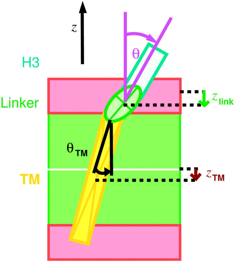
Reaction coordinates used for free-energy calculations, H3 helix tilt angle θ, TM helix tilt θ_TM, TM helix position z_TM, and linker position z_link. The red rectangles indicate the polar regions, the green rectangle the hydrophobic core of the bilayer.

For each observable x, the free-energy landscape G(x) was estimated from its distributions obtained from the room-temperature runs (Fig. 2, lower four blue boxes), excluding the first 3 ns as equilibration phase, as well as from ensembles of annealing final structures (red crosses in Fig. 4). To that end, an appropriate range [x_min, x_max] was divided into bins, where n is the number of available structures of the given ensemble. For the annealing ensembles, the range for θ was chosen as [0°, 120°], otherwise as the range of observed values. From the relative frequencies p_i of structures for which x falls into the i-th bin, an estimate for the (discretized) free-energy landscape,

(1)

was obtained, where x_i is the center of bin i, k_B the Boltzmann constant, and T the temperature. For the room-temperature ensembles, G(x_i) was smoothed by a Gaussian filter of the width of five bins standard deviation. Additionally, to estimate the associated stiffnesses from both the room temperature and the annealing ensembles, harmonic fits,

(2)

to the free-energy landscapes were obtained by computing average (equilibrium) values

(3)

and variances

(4)

of the observable x. Effective stiffnesses k were obtained from these harmonic fits via

(5)

Free energy of helix formation

For each linker residue i (i = 261,…,265), the probability p_i and free energy ΔG_i of helix formation was estimated as follows: Using the criteria of Kabsch and Sander for secondary structure elements (Kabsch and Sander, 1983), the number n_i of structures was determined for which one of the neighbors of the residue i was α-helical, and the number f_i of structures in which the residue i was α-helical itself. The free energy ΔG_i of helix formation was estimated via

(6)

with

(7)

Confidence intervals for annealing results

For the annealing results, due to their relatively small sample size, confidence intervals with confidence level 1 − α = 95% for the p_i were estimated from the Wilson score method (Wilson, 1927),

(8)

with α = Φ⁻¹(1 − α/2), and Φ denoting the error function. The upper and lower bounds of G_i, were obtained from Eq. 1 by replacing p_i by its bounds . The confidence intervals of ΔG_i were estimated similarly, here replacing n by n_i in Eq. 8. The confidence intervals [μ₋,μ₊] of μ were estimated from (E. Brunner, lecture note, Göttingen; C. Cenker, lecture note, Vienna)

(9)

where t_{n − 1,1 − α/2} is the (1 − α/2) quantile of Student's t-distribution with n − 1 degrees of freedom (Rohatgi and Saleh, 2001) (defined via (Rohatgi and Saleh, 2001)). The confidence intervals of σ were estimated as (E. Brunner, lecture notes; C. Cenker, lecture notes)

(10)

where χ_n−1,α/2² is the α/2 quantile of the χ_n−1² distribution (Rohatgi and Saleh, 2001).

Tilt energies

The energy necessary to tilt the H3 helix into its presumed orientation within the trans complex was estimated from

(11)

with θ = 80°. This angle was chosen somewhat smaller than 90° to account for the twist of the individual strands of the four-helix bundle with respect to the bundle axis. The parameters k and μ were obtained by harmonic fits to ensembles of simulated annealing final structures according to Eqs. 3 and 5. Confidence intervals [ΔE₋,ΔE₊] for a confidence level of 1 − α = 95% were estimated from the 1 − α percentile intervals obtained from a bootstrap (Efron and Tibshirani, 1993) run. Here, 5000 replica {θ^*}, each equal in size to the original sample {θ}, were generated by sampling with replacement from {θ} to obtain an empirical distribution of ΔE^* estimates. To verify that convergence was reached, varying numbers of replica were considered.

Significance of observed differences

To determine whether observed differences in estimated equilibrium tilt angles or stiffnesses are statistically significant, a bootstrap hypothesis test on the equality of means (Efron and Tibshirani, 1993) was applied. For samples {x}, 30,000 replica {x^*}, were generated by sampling without replacement from where μ denotes the mean value of the merged sample; hence an empirical distribution of the test quantity

(12)

was obtained. The fraction of t that exceeds the observed value yields the desired significance. For the equilibrium tilt angles, the test was applied to respective sample pairs {θ}, (bootstrap mean test); for stiffnesses, it was applied to the absolute deviations from the mean, {|θ − 〈θ〉|}, (bootstrap variance test).

For differences in the helicity of the individual linker residues, a modified bootstrap test for the equality of probabilities (bootstrap probability test) was devised: For two structure samples of sizes n₁ and n₂, let the studied residue be in helical conformation in k₁ and k₂ cases, respectively, yielding probability estimates p_i = k_i/n_i, i = 1,2. With the null hypothesis that the underlying probabilities are equal, p = (k₁ + k₂)/(n₁ + n₂) provides the best probability estimate. That estimate was subsequently used to generate bootstrap samples, thus yielding empirical distributions for k₁ and k₂ and, therefore, also for the test quantity t = |p₁ − p₂|. Hence the significance was estimated similarly as above.

Statistical independence of successive tilt angles

To check to what extent the H3 helix tilt angles θ_i and θ_i+1 of successive annealing start structures (Fig. 4, green circles) can be considered statistically independent, the (auto-) correlation coefficient r,

(13)

with and was calculated. The significance of the calculated correlation coefficients was assessed by a bootstrap correlation test for the null hypothesis of uncorrelated data. Bootstrap samples were generated by randomly permuting the θ_i, and the significance was estimated similarly as above from the obtained distribution of the test quantity t = |r|. A similar procedure was applied to the tilt angles of successive annealing final structures (Fig. 4, red crosses).

Hydrogen bonds

For the room temperature runs and for the final structures of each annealing set, the average number N_HB = 〈n_HB〉 of hydrogen bonds between the peptide (H3 and linker residues) and lipid headgroups was determined, as well as its fluctuation,

(14)

Here, n_HB denotes the the number of hydrogen bonds for each snapshot. Hydrogen bonds were counted if the distance between the hydrogen atom and the acceptor was below 2.5 Å and the angle between hydrogen atom, donor and acceptor was below 60°.

Additionally, for each set of n annealing final structures, the hydrogen bond probability p_i = k_i/n of each donor and acceptor i within the H3 helix and the linker was estimated by counting the number of structures k_i for which the respective hydrogen bond is detected. The significance α of differing p_i between two annealing sets was estimated using the bootstrap probability test.

Figs. 3, 6, 14, and 15 were prepared using MOLMOL (Koradi et al., 1996).

FIGURE 14.

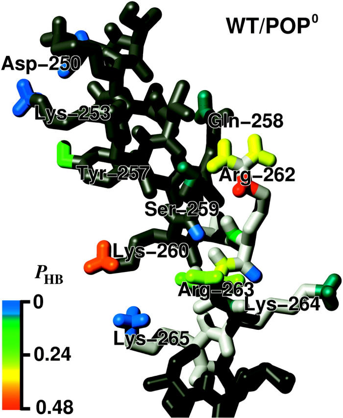
Color-coded probabilities p_HB of hydrogen bonds between the H3 helix (gray, top) or the linker region (light gray, mid), respectively, and adjacent lipid molecules (not shown). The structure is taken from the WT/POP⁰ annealing set (final structure) and is close to the average orientation. Part of the TM helix is shown in dark gray (bottom).

FIGURE 15.

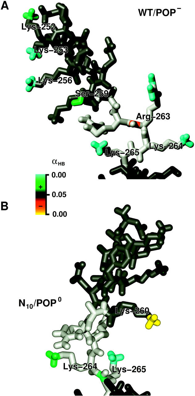
Color-coded significances (p-values) of hydrogen bond probability differences of WT/POP⁻ (top) and N₁₀/POP⁰ (bottom), compared to WT/POP⁰, denoting significant (p < 0.5) increase (green), confident (p ≈ 0) increase (cyan), significant decrease (red), and confident decrease (yellow), respectively, as determined by the bootstrap probability test. The structures are taken from the WT/POP⁻ and the N₁₀/POP⁰ annealing set, respectively, and are close to the respective average orientations. Atoms not involved in hydrogen bonding are shown in gray (H3 helix), light gray (linker), and dark gray (TM region).

RESULTS AND DISCUSSION

As can be seen in Fig. 3 (top), in the absence of a membrane, the solvated linker peptide used in the pilot study (Table 3, Set C) (initially modeled as a random coil) folded within 1.1 ns (trajectory WT^S/–/300 K), such that the H3 helix fragment contacted the TM helix fragment. Closer inspection revealed that the folding was driven by the hydrophobic contact between the H3-adjacent linker residue Ala-261 (orange) and the TM residue Ile-270 (yellow). The linker residues did not adopt any secondary structure. In contrast, when a simple membrane model was included (Fig. 3, bottom, red spheres), which mimicked the steric inaccessibility of the hydrophobic membrane core for the hydrophilic H3 helix (see Methods, trajectory WT^S/VdW/300K), the H3-adjacent linker residue Ala-261 spontaneously folded into α-helical conformation after ∼350 ps, as did Arg-262 after 400 ps (Fig. 3, black circle, bottom right). Also, the orientation of the H3 helix remained stable and parallel to the TM helix. The helical conformation of Arg-262 appeared to be only marginally stable and it unfolded again after 1.2 ns. The main conclusion from this pilot study is that the structure of the linker and the orientation and fluctuation of the H3 helix is presumably strongly affected by the presence of and interaction with the membrane. Therefore, a (computationally more expensive) explicit and accurate membrane model was used in all subsequent simulations.

Room temperature simulations

The linker structure obtained in the pilot study was used as the start structure for the preparation of the explicit bilayer system ( in Fig. 2). Fig. 6 shows the obtained system consisting of three turns of the H3 helix (cyan), the linker (red), and the full TM domain (yellow), embedded in a neutral lipid bilayer (POP⁰, green) composed of POPC and POPE molecules with an explicit solvent environment (water molecules are shown in blue).

Peptide insertion proceeded via an intermediate prosequence of 10 asparagine residues (N₁₀) that was appended at the C-terminus of the TM helix (magenta rectangle). As described in the Methods section, that prosequence was initially appended for the purely technical reason to avoid closure of the hole within the hydrophobic core of the bilayer, which was required to enable peptide insertion. During the subsequent free dynamics, the z-position of the peptide was expected to relax from its biased initial value toward a stable equilibrium. Indeed, a fast relaxation motion was seen during the first 40 ps, where the peptide penetrated the bilayer by further 2 Å (data not shown), and a slower relaxation by 2.5 Å in the same direction during the subsequent 450 ps. Remarkably, and in contrast to the simple membrane model used in the pilot study, during that time, the TM-adjacent linker residue Lys-265 folded into a stable α-helical conformation, presumably due to the increased hydrophobicity of the lipid headgroup region (Zhou and Schulten, 1995), which is described more realistically than in the pilot study. As will be analyzed in more detail below, this interaction is indeed quite complex. During the subsequent 1.4 ns, after a temporal backward movement, the peptide finally moved further toward the membrane center by 0.5 Å and reached a stable position, apparently independent of the chosen start position; for the next 3.2 ns, only a small drift is detectable, hence we assume the z-position of the TM helix to be close to equilibrium. The motion of the peptide brought the linker into the polar region of the bilayer. The TM helix, initially perpendicular to the bilayer, stabilized at tilts around 10°.

From the obtained simulation system, the start structures of the four main room temperature production runs were prepared (cf. Fig. 2; Table 3, Set A). For two of these (WT), the prosequence was removed, and 5 ns simulations for the neutral bilayer (POP⁰), composed of POPC and POPE, and a more physiological (Gennis, 1989) acidic bilayer (POP⁻), composed of POPC, POPE, and POPS, were carried out (trajectories WT/POP⁰/300K and WT/POP⁻/300K, respectively). For the other two simulations, the N₁₀ prosequence was kept.

Linker structure and stiffness

During the two WT simulations, two of the five linker residues remained in random coil configurations providing a hinge region between the H3 and the TM helix. Unexpectedly, already visual inspection of the trajectories suggested that the linker was quite stiff as opposed to, e.g., the highly flexible lipid tails. To quantify the stiffness, Fig. 7A shows the H3 helix tilt θ during the four simulations. For the neutral bilayer (POP⁰, blue curve), after ∼600 ps, the tilt angle stabilizes quickly at small values. For the acidic bilayer (POP⁻, green curve), the tilt angle starts at higher values and shows a slow drift, until, after 3 ns, it appears to be nearly equilibrated. We have therefore chosen the interval between 3 ns and 5 ns (gray) for the free-energy estimates according to Eq. 1.

FIGURE 7.

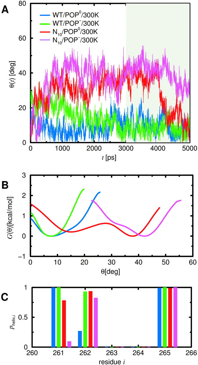
(A) Tilt angle θ of the H3 helix with respect to the bilayer normal during room-temperature free-dynamics runs of the wild-type (WT) and the prosequence mutant (N₁₀), both embedded within uncharged (POP⁰) and charged (POP⁻) bilayer. The period that was used for the free-energy landscape estimate, G(θ), is shaded gray. (B) Smoothed free-energy landscape for the H3 helix tilt angle, derived from the four free-dynamics runs of 2-ns length each, according to Eq. 1. (C) Linker helicities determined from the four 2-ns free-dynamics runs. Shown are the relative frequencies p_helix,i that each of the five linker residues is in helical configuration, given that one of its neighbors is helical.

The obtained free-energy landscapes are shown in Fig. 7 B. Both WT simulations show a narrow energy minimum located at small angles (blue and green curves); angles larger than 25° are rarely encountered. Accordingly, the H3 helix remains nearly parallel to the bilayer normal with a small average tilt angle and considerable tilt stiffness. To quantify these two properties, a harmonic potential (Eq. 2) was fitted to the observed ensemble of tilt angles θ using Eqs. 3 and 5 yielding an equilibrium angle θ₀ and an effective stiffness k_θ (see Table 4). Whereas the equilibrium angles are similar for the two WT simulations, the additional charges of the acidic bilayer (POP⁻) seem to increase the stiffness of the linker by a factor of two.

TABLE 4.

Parameters of harmonic fits

System	θ0	kθ	θTM,0	kθ,TM	zlink,0	kz,link	zTM,0	kz,TM
WT/POP0	9.9	25	16.7	71	−5.4	4.9	−3.8	4.7
WT/POP−	8.1	50	12.9	74	−4.4	2.9	−3.0	4.0
N10/POP0	27.2	4.2	16.7	59	−0.03	2.6	0.75	3.1
N10/POP−	40	17	19.3	95	−1.7	3.7	−0.61	6.4

Parameters for H3 helix tilt (θ₀, k_θ), TM helix tilt (θ_TM,0, k_θ,TM), linker position (z_link,0, k_z,link), and TM helix position (z_TM,0, k_z,TM), as estimated by Eqs. 3 and 5. For θ and θ_TM, the equilibrium values are given in degrees and the force constants in 10⁻³ kcal mol⁻¹ deg⁻². For z_link and z_TM, the equilibrium values are given in Å and the force constants in kcal mol⁻¹ Å⁻². The definition of the observables is sketched in Fig. 5; the systems are listed in Table 3.

Effects of acidic lipids

To check if the increased stiffness for POP⁻ coincides with an increased linker helicity, the conditional probability p_i of helix formation in the presence of a helical neighbor residue was estimated for each linker residue i using Eq. 7 (Fig. 7 C). As can be seen, residues Ala-261 and Lys-265 are in a stable helical conformation for both bilayer types, whereas Arg-263 and Lys-264 remain in a random coil conformation. The only—albeit very pronounced—difference is seen for Arg-262, which is helical for POP⁻, but only marginally so for POP⁰. This suggests that the larger stiffness is caused by the increased helicity, which, in turn, is induced by the lipid charges. In particular, changing a single residue into helical configuration can increase the tilt stiffness of the H3 helix considerably.

Effects of prolongation

Unexpectedly, the tilt angle behaved quite differently already in the run, which led us to suspect that the prosequence has a pronounced impact on the mechanical properties of the linker—despite the considerable distance between prosequence and linker region. Therefore we also carried out 5-ns simulations of the mutant both for neutral and for the acidic bilayer (Fig. 7 A, red, magenta). Indeed, even though they start at small tilt angles, both systems show much larger angles and larger fluctuations already after 800 ps compared to the WT. Straightforward calculation of the respective free-energy landscapes is complicated, due to the notorious sampling problem. In particular, the system (red) jumps back to smaller angles after 4.2 ns and remains in that (metastable) state for the remaining simulation, such that, due to insufficient statistics, the computed free-energy landscapes (Fig. 7 B) have to be judged with care. In particular, the relative height of the two apparent minima cannot be estimated unless multiple transitions are observed. In the second part of the Results section, this problem will be approached more systematically by multiple simulated annealing runs.

Table 4 summarizes the results of the—in this case necessarily rough—harmonic fits to the ensembles of N₁₀ tilt angles. As can be seen, for the neutral bilayer, the average tilt angle of the linker of the mutant is about three times larger than that of the WT, whereas the stiffness decreased by a factor of five—mainly due to the fact that two metastable states are encountered. For the acidic bilayer, an even larger (by a factor of four with respect to the WT) average tilt is seen and the stiffness is about three times smaller. Although the individual fit parameters are likely not very accurate at the present stage of analysis, the qualitative difference between the mutant and the WT is evident and thus deserves closer inspection.

Also for the mutant, the level of helicity was studied as possible cause for the changed stiffness (Fig. 7 C, red, magenta). As can be seen, for both bilayer types the conformations of Arg-263, Lys-264, and Lys-265 are similar to the WT systems. In contrast, the quite stable helical conformation of Ala-261 for the WT systems is destabilized for both bilayer types, particularly for N₁₀/POP⁻ (magenta), which also showed the largest average tilt. Apparently, the helicity of Ala-261 and hence the stability of the backbone hydrogen bond between Ala-261 and Tyr-257 is a critical determinant for the spontaneous H3 helix tilt. The observed correlation is also seen in the time domain, e.g., for N₁₀/POP⁰. Here, the pronounced and abrupt decrease of the tilt angle from ∼40° to 15° at 4200 ps (Fig. 7 A, red curve) followed a transition of Ala-261 from an equilibrium between helical and nonhelical conformation to a stable helical one at 3070 ps where it remained for the rest of the trajectory. Also, at 3200 ps, Arg-262 folded into a stable helical conformation, which, for the WT, was shown to be crucial for the H3 helix tilt stiffness. Moreover, the observed sequence of events in this case rules out the possibility that helix formation is the consequence of tilt angle changes rather than their cause. Although an (unknown) common cause can not be strictly ruled out, we attribute for both mutant systems the increased average tilt and decreased tilt stiffness to the reduced linker helicity.

Linker embedding

The previous result that inclusion of a realistic membrane environment can change the helical content of the linker suggested a mechanism for the initially unexpected long-distance impact of the prolongation: By changing the z-position of the TM helix, the prolongation could expose the linker region to a more hydrophilic environment and thereby destabilize the backbone hydrogen bond between Ala-261 and Tyr-257, which, in turn, affects the mechanical properties of the linker. To check this hypothesis, for all four systems the vertical linker position z_link with respect to the average positions of the phosphor atoms of the proximate polar region (see Fig. 5) was monitored and the respective free-energy landscapes were determined using Eq. 1. As can be seen in Fig. 8 A, and also from the harmonic fits listed in Table 4 (z_link,0, k_z,link), all four systems exhibit narrow energy minima; accordingly, the linker position is well-defined. As expected, the position of the WT (blue, green) is generally shifted with respect to that of the mutant (red, magenta) in such a way that the linker becomes buried deeper within the membrane, which supports our hypothesis. The effect is particularly strong for the neutral bilayer with a shift of 5.4 Å and less pronounced for the charged bilayer with a shift of 2.7 Å. Interestingly, compared to the neutral bilayer, the lipid charges shift the linker positions of WT and mutant in opposite directions by ∼1 Å. As shown in Table 4, for N₁₀ the linker is located roughly at the z-position of the phosphate groups. For WT, the linker resides unexpectedly deep in the membrane, suggesting that the membrane environment strongly influences the linker properties in this case.

FIGURE 8.

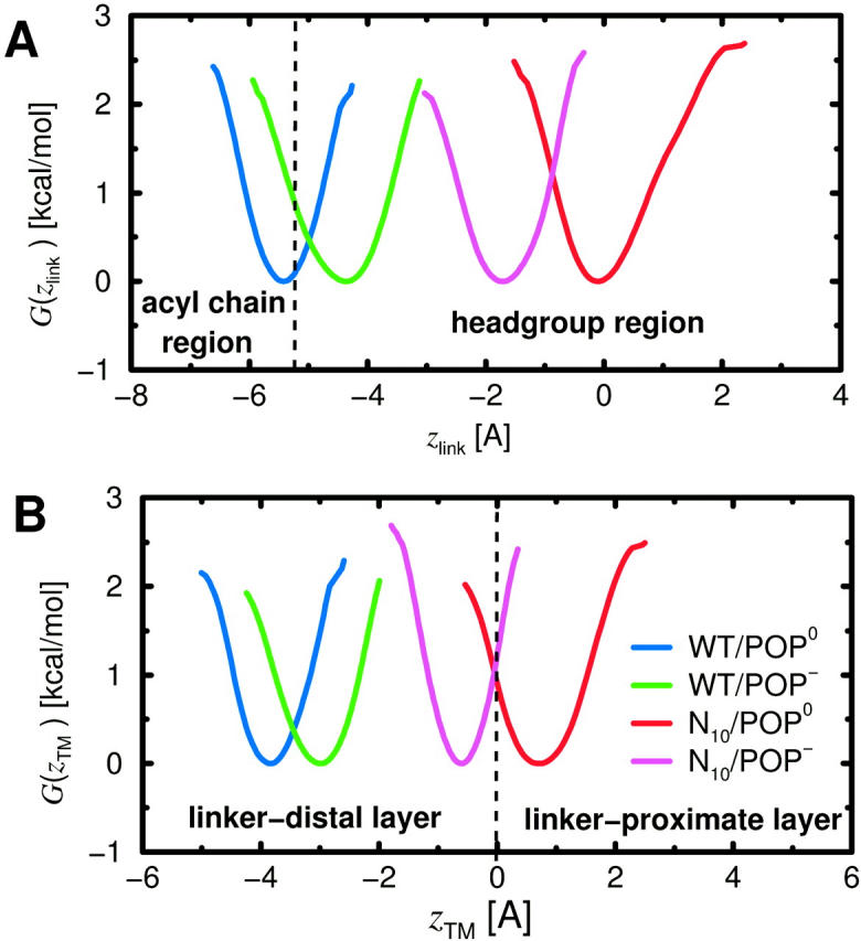
Smoothed free-energy landscapes (A) for the linker position z_link with respect to phosphate groups and (B) for the position z_TM of the TM helix center with respect to membrane center (dashed line), both derived from the four free-dynamics runs of 2 ns length according to Eq. 1. In A, the polar region is indicated, here defined via the distribution of phosphate group positions, using a cutoff (dashed line) at two standard deviations around the average position (Zhou and Schulten, 1995).

For POP⁻, the difference of z_link,0 between WT and N₁₀ is decreased as compared to the respective POP⁰ systems by a shift of 1 Å for WT and a shift of 1.7 Å for N₁₀ (see Table 4) toward intermediate values. This may reflect strong electrostatic interactions between the basic linker residues and acidic lipids that should be strongest near a particular linker position z_link,el. This position apparently resides between the equilibrium positions of WT/POP⁻ and N₁₀/POP⁻, presumably closer to the value for WT/POP⁻, as judged from the lower shift induced by the lipid charges for WT; i.e., z_link,el, ≤ −3 Å.

Hydrogen bonds

Generally, the lipid charges are expected to strengthen the interactions between the lipids and the peptide. On the other hand, the prolongation, reducing the peptide penetration, may weaken the peptide-lipid interactions (and thereby increase tilt flexibility). To check these hypotheses, the average number of hydrogen bonds between linker and H3 domain to surrounding lipid molecules, as well as its fluctuations (Eq. 14), were determined for each system. As shown in Fig. 9, as anticipated, the POP⁻ systems show more frequent hydrogen bonding than the respective POP⁰ systems. This may contribute to the increased tilt stiffness observed for the POP⁻ systems. For POP⁻, a small decrease in the number of hydrogen bonds for N₁₀, as compared to WT, can be observed. For POP⁰, unexpectedly, the average number of hydrogen bonds between peptide and lipids does not strongly differ between WT and N₁₀.

FIGURE 9.

Average number N_HB of hydrogen bonds between the peptide (H3 and linker residues) and lipid headgroups determined from production phases of free-dynamics runs and from ensembles of annealing final structures. The bars denote fluctuations (Eq. 14). Note that the error bars are much smaller than the fluctuations.

Hydrophobic anchoring of the TM helix

That the observed shifts of the linker z-position are actually due to a shifted TM helix is evident from Fig. 8 B, which shows the free-energy landscape for position of the TM helix center measured with respect to the membrane center (cf. also Fig. 5). Indeed, the close similarity of Fig. 8, B and A, confirms that the TM domain is nearly rigid such that, as expected, the position of the TM helix within the bilayer determines that of the linker. Remarkably, the hydrophobic TM helix is optimally centered within the hydrophobic region of the bilayer (z_TM ≈ 0) only for the mutant, whereas it is shifted out of this symmetrical position by 4 Å for the WT. Apparently, the system trades off partial hydrophobic mismatch of the TM helix and the linker with the need to fill the hole in the distal lipid headgroup region, which would be present for the symmetrical TM position. Therefore we assume that also many other hydrophilic prosequences with different structures would have similar effects as the one chosen here initially for purely technical reasons.

Table 4 lists the average positions z_TM,0 and stiffnesses k_z,TM obtained from harmonic fits for the TM positions. As can be seen from the table, as well as from Fig. 8 B, also the mutant, anchored in the neutral bilayer, is slightly shifted out of the symmetric position in the inverse direction by ∼1 Å. One likely reason is the sequence asymmetry between linker and prosequence and, in particular, the presence of the four positive charges of the linker. That the asymmetry is inverted for the acidic bilayer, which changes the electrostatic environment of the linker, further supports the relevance of the interaction between linker and lipid headgroup region discussed above. The stiffnesses are, overall, very large, corresponding to a force of ∼300 pN for a 1-Å deflection. Such stiffness is actually indispensable for the proposed membrane fusion mechanism, because it is required to keep the peptide tightly anchored within the bilayer, so that it can withstand the strong repulsion forces that occur when two membranes are pulled toward each other.

TM helix tilt and structure

The second important requirement, as mentioned in the introduction, is that the TM helix must be able to withstand tilting with respect to the membrane normal. To study if this actually is the case, free-energy landscapes also have been computed from the simulations for the TM tilt angle θ_TM (see Fig. 5). Within the equilibration phase of the simulation that angle departed from its initially chosen value of 0° toward values around 10° (data not shown). The minima of the free-energy landscapes (see Fig. 10) are significantly narrower than those of G(θ), indicating that θ_TM is more strongly restrained than θ. Table 4 lists the corresponding average tilts θ_TM,0 and the tilt stiffnesses k_θ,TM obtained from harmonic fits. Overall, the stiffnesses of the TM helix angle are larger than the ones of the linker angle, such that the mechanics should be mainly determined by the stiffness of the linker.

FIGURE 10.

Free-energy landscapes of TM helix tilt θ_TM with respect to the membrane normal from room temperature production runs.

Both the TM domain and the prosequence were initially modeled in α-helical configuration. To check if this configuration is maintained during the free-dynamics runs, the secondary structures of the TM domain (residues 266–288) and of the prosequence (residues 289–298) were monitored (data not shown). For WT/POP⁰, the TM residues 266–286 remained helical, and only the C-terminal residues Phe-287 and Gly-288 adopted a random coil configuration. Also WT/POP⁻ remained helical; here only residue Gly-288 adopted a random coil configuration. Apparently, as for the linker residues, the lipid charges also increased the helicity of the TM C-terminus. For the N₁₀ systems, due to the juxtaposed prosequence, the entire TM domain remained α-helical for both lipid types. Also residues 289–294 of the prosequence showed a stable helix conformation; residues 295–296 were only marginally helical, and residues 297–298 adopted a random coil conformation. For N₁₀/POP⁻, the helicity of residue Asn-296 was increased with respect to N₁₀/POP⁰, thus providing a further example that the charged bilayer tends to stabilize helical conformations. Although the remaining helical structure of the prosequence was stable during the two 5-ns production runs, no solid evidence can be provided that this would also be true for longer timescales. The main effect of the (hydrophilic) prosequence to drag the (hydrophobic) TM domain into a centered position should, however, not critically depend on the helical structure of the prosequence and therefore the predicted effect on the mechanical properties of the linker should be observable in experiments.

Simulated annealing runs

Concerning the linker structure and tilt angle, the room-temperature simulations suffer from an apparent sampling problem, as can be seen, e.g., from the fact that only one transition is seen for N₁₀/POP⁰ (Fig. 7 A, red). Also, the physiological membrane fusion timescales are likely three orders of magnitude longer than the nanosecond simulation times (Cevc and Richardsen, 1999). Thus it is unclear as to what extent the linker structures seen in the simulations could be biased by the chosen start structure. Moreover, also the calculated average tilt angles and, in particular, the stiffnesses may be inaccurate due to insufficient sampling.

To reduce this problem and to improve the sampling, we have carried out high-temperature runs followed by multiple simulated annealing runs (Fig. 2, red boxes). For both the WT and the mutant, 1-ns high-temperature runs were carried out at 1500 K as described in the Methods section starting from the respective production run trajectories (black arrows). For the WT in the neutral bilayer, three different cooling rates were used to assess convergence. As also described in the Methods section, the TM helix and the lipid tails had to be restrained for the high-temperature and annealing runs to avoid degradation of the system. For the successive free-dynamics room-temperature runs, the restraints were removed. Inasmuch as z_TM and θ_TM are much better sampled and show only small fluctuations as compared to the H3 helix tilt angle (cf. Figs. 8 A and 10), we do not expect these restraints to severely limit the sampling of the linker structure and the linker tilt angle. In particular, results from recent measurements on the membrane immersion of the syntaxin linker are consistent with our results of the average linker position and in this regard support our assumptions (Kweon et al., 2002).

Fig. 11 A shows the results of a set of WT/POP⁰ annealing runs (cf. Fig. 4) compared with the respective room-temperature production trajectory (blue). Rather than the tilt angle θ, here the projection of the (normalized) H3 helix axis onto the xy bilayer plane has been plotted; the center corresponds to θ = 0°. As can be seen, the 1-ns 1500-K sampling run (brown dots) provided a much broader distribution of H3 helix orientations than the 2-ns room-temperature production phase. Furthermore, the region covered by the room-temperature run is only rarely visited within the sampling run, suggesting that the free energy of other regions is lower, at least at this high temperature. This finding can be explained by the fact that the distributions of H3 helix orientations are governed by respective free energy landscapes, G = H − TS, which, in addition to the enthalpic contribution H, also include temperature-dependent entropic contributions, −TS, which generally tend to widen the distribution for increased temperatures.

FIGURE 11.

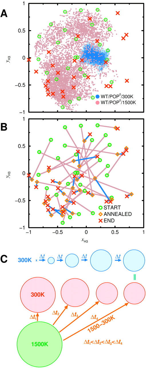
Projection of WT/POP⁰ H3 helix orientations (unit vectors) onto the xy bilayer plane; the azimuth is plotted relative to the TM helix. (A) 2-ns room temperature trajectory (blue), high-temperature trajectory (brown), selected annealing start structures (green), and obtained annealing and free-dynamics final structures (red). (B) Distances traversed during individual annealing (brown) and equilibration (blue) phases. (C) Sketch of expected convergence behavior of room-temperature dynamics and simulated annealing distributions. The circles symbolize distributions of H3 helix orientations, in a similar representation as A. See text for explanations.

Convergence

To approximate the room-temperature distribution of interest, 27 uniformly distributed structures (green circles) were selected from the high-temperature trajectory. Each of these was annealed to room temperature during 400 ps and subsequently subjected to free dynamics for 200 ps. In Fig. 11 A, the obtained final structures are shown in red. The distances traversed during these two steps are shown in Fig. 11 B (brown, blue). If both the room-temperature sampling and the relaxation during the annealing and subsequent room-temperature runs were complete, the distribution of final structures (red) and of the room-temperature trajectory (blue) should agree. In contrast, the annealing final structures show a relatively broad distribution with clusters similar to the high-temperature distribution (e.g., within the lower left corner). Also several outliers are seen in regions that were not covered from the high-temperature sampling run. Two or three structures reside within the region sampled by the room-temperature run.

Fig. 11 C provides a possible explanation for these findings. With increasing simulation time (multiples of Δt), the room-temperature distribution tends to broaden (and may also shift position), as indicated by the blue areas, as increasing volumes in the configuration space are sampled. Eventually, if the simulation time were long enough for sufficient sampling, the distribution would converge toward the equilibrium distribution (right). Thus, insufficient sampling typically underestimates the width of the equilibrium distribution and therefore yields an upper limit for the stiffness of the underlying effective potential. In contrast, and assuming that the sampling during the high-temperature run is nearly complete, the obtained distribution (green area) will typically be broader than the equilibrium distribution due to the dominance of the entropic contribution to the underlying free-energy landscape. This will also be true for the final structures of very short (Δt₁) annealing runs (red area, left) that started from structures taken from the high-temperature ensemble. The structures cannot relax toward their room-temperature equilibrium and rather get trapped in local energy minima. With increasing annealing period Δt₁, Δt₂, Δt₃, Δt₄, increasingly complete relaxation takes place, and the width of the distribution narrows. For very long annealing periods, it would converge toward its equilibrium value (right). Thus, for annealing, the equilibrium width will typically be approached from above, which should yield a lower limit for the stiffness of the underlying effective potential.

To check if this setting applies for the case at hand, annealing sets with varying annealing periods (t = 400, 800, 1600 ps; cf. Fig. 2) were created. From the resulting sets of final structures, free-energy landscapes were determined as described in the Methods section. In contrast to the 5000 structures obtained from the room-temperature ensembles, the annealing final sets provided only 27 structures each, thus limiting the accuracy and resolution of the obtained energy landscapes. But whereas subsequent annealing final structures should, by construction, be hardly correlated (unlike subsequent structures from normal MD trajectories, which are highly correlated), accurate confidence intervals for the free energies can be calculated, using Eqs. 8 and 1.

Linker stiffness

Fig. 12 A shows the resulting free-energy landscapes (red, blue, and green) for the three different annealing periods, together with 95% confidence intervals. Additionally, to detect a possible bias by the chosen linker start structure, a fourth energy curve (orange) has been calculated from a separate series of simulations (Fig. 2, top row), which started with the linker in fully helical configuration. Overall, the energy minima show similar widths and tilt angles that are both considerably larger than those derived from the room-temperature free-dynamics run (brown). Fig. 12 B depicts these values as calculated, like the ones for the room temperature runs, from harmonic fits. Assuming uncorrelated data, 95% confidence intervals were estimated for θ₀ from Eq. 9 and for k_θ from Eqs. 10 and 5 and are also shown in Fig. 12 B.

FIGURE 12.

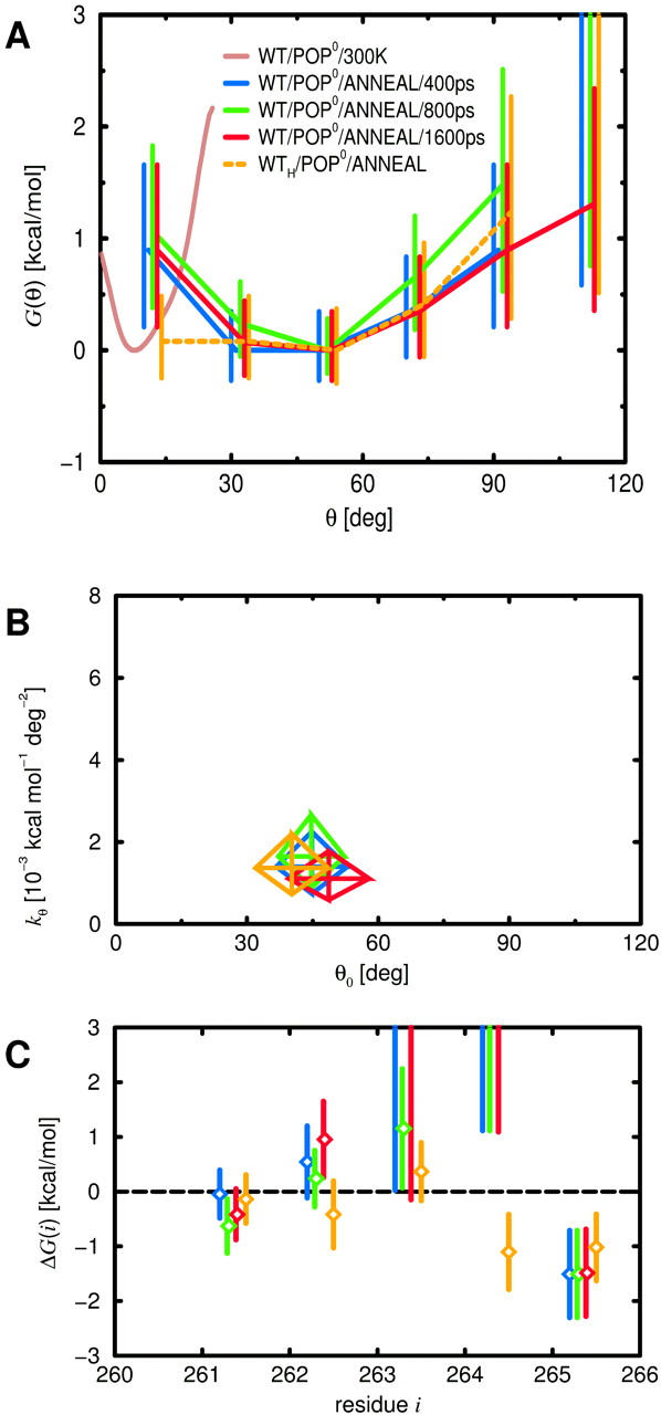
Influence of annealing lengths (blue, green, red), as well as partly and fully helical linker start structure (blue, orange) on structure and mechanical properties of the linker for WT/POP⁰, obtained from the final structures of respective simulated annealing sets. (A) Free-energy landscapes for H3 helix tilt estimated using Eq. 1, with 95% confidence intervals from Eq. 8; for comparison, the free-energy landscape obtained from the room-temperature simulations is also shown (brown). (B) Parameters θ₀ and k_θ of harmonic fits to H3 helix tilt θ; the centers of the rhombi indicate estimates according to Eqs. 3 and 5, the diagonals 95% confidence intervals for θ₀ (Eq. 9) and k_θ (Eq. 10). (C) Free energy of helix formation as estimated from Eq. 6, with 95% confidence intervals as estimated from Eqs. 8 and 6.

As expected, increasing the annealing period from 400 ps (blue curve) to 800 ps (green curve) narrowed the derived-energy landscape. However, a further increase to 1600 ps (red curve) broadens the width of the distribution to even above the 400-ps value. One possible explanation is that the sampling during the high-temperature run was insufficient and, therefore, is further improved during the annealing runs; the resulting broadening of the distribution could partially compensate the originally expected narrowing. The annealing final structure outliers (Fig. 11 A, red) could in fact indicate regions that were accessible but not reached during the high-temperature sampling run. However, the large overlap of the error bars in Fig. 12, A and B, suggests, at this point of analysis, statistical fluctuations as the more likely explanation. Indeed, when estimated using the bootstrap mean and variance test, respectively, the significances of the pairwise differences for θ₀ and k_θ (Table 5, left two columns) turn out to be rather low (i.e., large p-values) for the three different annealing lengths (upper three rows). In this case, the mechanical linker properties obtained from the annealing sets may either be already close to their equilibrium values, or alternatively, their convergence might be so slow that even for an increase of the sampling time by a factor of four, no improvement can be detected.

TABLE 5.

Significances of H3 helix tilt and linker helicity differences

tcool,1	↔	tcool,2	θ0	kθ	p261	p262	p263	p264	p265
400	↔	800	0.98	0.61	0.13	0.51	0.63	1.00	1.00
800	↔	1600	0.49	0.33	0.66	0.12	0.63	1.00	0.91
400	↔	1600	0.52	0.62	0.26	0.46	1.00	1.00	0.91
WT/POP0	↔	WTH/POP0	0.42	0.67	0.74	0.04	0.19	0.00	0.35
WT/POP0	↔	WT/POP−	0.02	0.03	0.13	0.00	0.61	1.00	0.03
WT/POP0	↔	N10/POP0	0.20	0.55	0.32	0.59	0.30	0.01	0.00

Respective p-values for various pairs of annealing sets, as estimated by applying the appropriate bootstrap hypothesis tests described in the Methods section. The mean test was used for the spontaneous tilt θ₀, the variance test for the tilt stiffness k_θ, the probability test for helicity p_i of residue i (i = 261,…,265). The upper three lines list pairs obtained for system WT/POP⁰ with various annealing lengths; the lower three lines list comparisons of the 400 ps WT/POP⁰ annealing set with the specified sets.

In summary, the stiffness values shown in Fig. 12 B provide a lower limit for the tilt stiffness, which is smaller than the upper limit obtained from the room-temperature run by a factor of 15. We note that also the values for the other stiffnesses listed in Table 4 represent, in principle, upper limits. For k_θ,TM, k_z,link, and k_z,TM, however, we have already seen above that the sampling is expected to be nearly complete, so that the obtained values should already be close to their equilibrium values. Therefore, no additional simulated annealing runs have been carried out for these observables.

The average tilt angle θ₀ (∼40°) obtained from the annealing runs is four times larger than the one obtained from the room-temperature run. We attribute this difference to an entropic effect: For given tilt interval centers at θ, the accessible solid angle increases with θ as sin θ, implying larger entropy. Thus, for higher temperatures, the minimum of the free-energy landscape tends to move to larger tilt angles, which may not fully relax to the room-temperature values during annealing. Therefore, we consider it likely that the average tilt angle for the WT is smaller than 40°.

Note finally that H3 helix tilt angles above 90° are rarely obtained for annealing runs, which give rise to the finite free-energy values at 105° in Fig. 12 A. Under physiological conditions, the presence of the cytosolic core complex, which is not included in our simulations, prohibits such large tilts.

Linker structure

To characterize the linker structure, for each linker residue i, the probability p_i and the free energy ΔG_i of helix formation were estimated from the ensembles of final structures of different annealing sets using Eq. 6. Assuming uncorrelated data, confidence intervals were determined from Eqs. 8 and 6. As shown in Fig. 12 C, the annealing yielded a quite similar helicity pattern as the one obtained from the respective room-temperature run (Fig. 7 C, blue bars). An exception is Ala-261, which was helical in the room-temperature run but only marginally so for the annealing sets. Given the large difference in G(θ) between the room-temperature and annealing sets, the fact that only a single amino acid is affected is remarkable. The results obtained for WT/POP⁰ and N₁₀/POP⁰, however, reveal a similar trend, namely that reduced helicity of Ala-261 implies increased average angle θ₀ and reduced tilt stiffness k_θ. Moreover, the change in helicity between WT/POP⁰ and N₁₀/POP⁰ is smaller for the room-temperature simulations than for the annealing runs and so is the change in the mechanical properties of the linker (see below).

The linker properties obtained from annealing sets of varying length were found to change only slightly. However, also here, comparison of Ala-261 helicity (Fig. 12 C, left) with the tilt parameters (Fig. 12 B) reveals the same trend as seen above. Some of the individual p-values for the difference in helicity of Ala-261 and Arg-262 (Table 5) show even larger significances (albeit still above the 5% level) than those for the tilt parameters. Moreover, the helicities of Arg-262 and Arg-263 also follow this trend, so that the joint significance should be well below 5%. Overall, the helicities of the individual linker residues are a more sensitive indicator for changes in the simulation setup than the mechanical properties of the linker.

As seen for the linker parameters (Fig. 12 B), the helicities also show no monotonous variation with the length of the annealing periods, presumably for similar reasons, namely a near compensation of the effects of enhanced high-temperature sampling (which decreases the helicity) and of improved low-temperature relaxation (which increases the helicity). Because the helicities of all three linker residues (Ala-261, Arg-262, and Arg-263) increase from WT/POP⁰/ANNEAL/400ps to WT/POP⁰/ANNEAL/800ps, whereas they collectively decrease from WT/POP⁰/ANNEAL/800ps to WT/POP⁰/ANNEAL/1600ps, the former change is likely dominated by improved relaxation and the latter by enhanced sampling. We note that the same was seen for the mechanical properties of the linker, which renders it unlikely that these results are purely due to statistical fluctuations and thus substantiates the compensation argument tentatively given above.

That the helicities obtained from the room-temperature simulations and the ones from the annealing sets are strikingly similar can have two reasons. First, both approaches could yield structures close to equilibrium; second, there may be a bias due to the chosen (nonhelical) start structure. The simulations starting with fully helical linker conformation served to detect such possible bias (Table 3, Set B, second system). The initial room-temperature equilibration run (WT_H/POP⁰/300K, see Fig. 2) showed transitions to random coil and back to helical configurations (data not shown). Fig. 12 C shows the helicities obtained from the subsequent annealing set (orange). Comparison to WT/POP⁰/ANNEAL (blue) shows a significantly increased helicity particularly for Lys-264 (see Table 5 for the respective p-value), which renders a certain bias due to the chosen start structure indeed very likely for this residue. A small influence is also seen for Arg-262 and Arg-263. Nearly unaffected by that possible bias are the other helicities and, most importantly, the energy landscape for the tilt angle, G(θ), (Fig. 12 A, orange) and hence also the linker tilt stiffness k_θ (cf. Fig. 12 B). This finding confirms the previous observation that the mechanical properties of the linker are mainly determined by the conformation of Ala-261 and underscores the reliability of the stiffness estimates.

We note that the confidence intervals and significance estimates discussed above rely on the assumption of uncorrelated samples. To check this assumption, for each annealing set (see Fig. 4), the correlation of subsequent start structures (green) and final structures (red) was estimated using Eq. 13, as well as the significance of this correlation using the bootstrap correlation test (Table 6). Indeed, WT/POP⁰ turns out to be nearly uncorrelated whereas WT_H/POP⁰ does show significant correlations for both start and final structures. We attribute these correlations to the increased linker helicity, which can slow down the dynamics of the H3 helix tilt angles. Because the observed correlations of ∼0.5 reduce the respective effective sample size by roughly a factor of two, the confidence intervals and p-values calculated above are actually larger by a factor of ∼ That effect reduces the bias discussed above somewhat.

TABLE 6.

Correlations of H3 tilt angles

System	rs	ps	re	pe
WT/POP0	0.13	0.52	0.12	0.65
WTH/POP0	0.77	0.00	0.28	0.19
WT/POP−	0.39	0.07	−0.34	0.08
N10/POP0	0.44	0.02	0.47	0.01

Correlations of tilt angles from subsequent start (r_s) and end structures (r_e) from four different annealing sets (Eq. 13) and respective p-values estimated from the bootstrap correlation test.

To summarize the main results obtained so far from the annealing runs, for the WT embedded within neutral bilayer, the linker is helical at its termini with decreasing helicity toward the linker center. As evident from Fig. 12 A and using Eq. 11, an energy of ∼0.9 kcal/mol (with 95% confidence interval [0.5, 1.8] kcal/mol) is required to tilt the linker to 80°, which is the angle expected for fully assembled trans complex geometry.

Effects of acidic lipids

To study the effect of lipid composition on the mechanical properties of the linker, a set of high-temperature and annealing runs was carried out also for system WT/POP⁻/SALT (WT/POP⁻/ANNEAL, see respective red box in Fig. 2). The obtained energy landscape for the H3 helix tilt angle (Fig. 13 A, green curve) shows, compared to WT/POP⁰ (blue curve), a very steep minimum, which is located at a large tilt angle. The parameters of the harmonic fit (see Fig. 13 B, green rhombus) quantify this effect. The tilt stiffness k_θ is larger by a factor of ∼2.5, which confirms the increase by a factor of two that was already obtained from the room-temperature simulations (see Table 4). As compared to WT/POP⁰ (blue rhombus), the average tilt angle θ₀ is larger by 15°. Table 5 shows that this effect of the lipid charges on the linker properties is significant.

FIGURE 13.

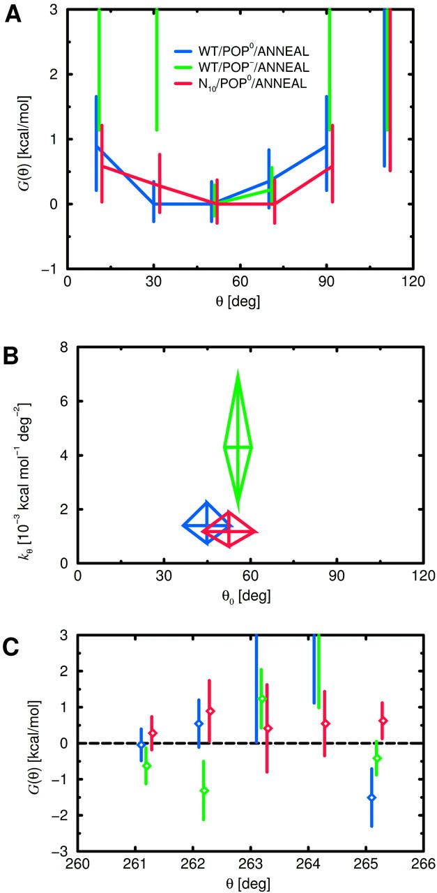
Structure and mechanical properties of the linker for WT embedded in POP⁰ (blue) and POP⁻ (green), as well as for N₁₀/POP⁰ (red). (A) Free energy of H3 helix tilt angles. (B) Spontaneous H3 helix tilt θ₀ and tilt stiffness k_θ. (C) Free energy of helix formation.

These tilt property changes are related to changes in linker structure as shown in Fig. 13 C (green symbols). Similar to the room temperature runs (Fig. 7 C, green bars), as compared to WT/POP⁰ (blue symbols), the helicity of Arg-262 is significantly increased. The helicity of Ala-261 is also larger whereas that of Lys-265 is smaller, in agreement with the room-temperature simulations. The latter may be explained by the reduced peptide penetration (by ∼1 Å) seen for the charged bilayer system with respect to the neutral bilayer (data not shown). Table 4 shows that this effect is insensitive to salt concentration. This could mean that the larger average tilt angle is due to the changed conformation of Lys-265 and that the larger helicity of Ala-261 and Arg-262 dominates the stiffness increase of the linker. To substantiate this assumption, the interactions between the peptide and the adjacent lipids were analyzed in detail (see below).

In light of the conformational coupling assumption, the increase of θ₀ is expected to reduce fusion efficiency whereas the increase of k_θ should have the opposite effect. To judge which of the two effects dominates, the energy necessary to tilt the H3 helix to the 80° expected for the fully assembled trans complex was estimated. Compared to POP⁰, a slightly increased tilt energy of 1.2 kcal/mol was obtained with a confidence interval of [0.8, 2.4] kcal/mol, which suggests an increased fusion efficiency. Unfortunately, due to the overlapping error bars, the significance of this is low, and a null effect, therefore, cannot be ruled out with certainty.

Effects of prolongation

A set of high-temperature and annealing runs was carried out also for system N₁₀/POP⁰ to study the effect of the prosequence on the linker stiffness (see Fig. 2). Here, the main effect is a shift of the obtained energy landscape for the tilt angle to larger values (Fig. 13 A, red curve) as compared to WT/POP⁰ (blue curve). This is reflected in the increased average tilt angle obtained from the harmonic fit (Fig. 13 B, red), which was also seen for the room-temperature simulations. The tilt stiffness is unchanged.

The relation between decreased helicity of Lys-265 (Fig. 13 C, red) and increased average tilt follows the same pattern as seen for the charged bilayer and therefore provides a plausible cause of the increased tilt. Furthermore, the helicity of Ala-261 is also reduced with respect to the WT (neutral bilayer), albeit with only little significance (see Table 5). On the contrary, the helicity of Lys-264 and, to a smaller extent, that of Arg-263 became larger.

Overall, the helix is significantly weakened at the linker ends and stabilized for the central residues. Here, the change of the linker environment is solely due to the reduced peptide penetration (Fig. 8 A, red curve) rather than the charged bilayer but has an even larger effect on the structure of the linker. Table 6 lists the correlations of subsequent annealing structures that fall into the range discussed for the other annealing sets with similar implications for the confidence intervals and p-values.

Qualitatively, the changes of the linker structure seen in the annealing runs confirm and extend those of the room-temperature simulations. In the context of the conformational coupling assumption, the energy required to tilt the H3 helix into trans complex configuration of 0.4 kcal/mol ([0.2, 0.8] kcal/mol) is considerably reduced with respect to the WT by more than a factor of two, which suggests a correspondingly reduced fusion rate.

Hydrogen bonds

To further characterize the interaction between the peptide and its environment, the average numbers N_HB of hydrogen bonds between H3 helix/linker residues and adjacent lipid molecules, as well as the respective fluctuations, were determined for the final structures of the three annealing sets discussed above. As can be seen in Fig. 9 (black symbols), N_HB increased by a factor of two for each system with respect to the room-temperature runs. In particular, many of these additional hydrogen bonds are formed by the H3 helix due to the occurrence of large helix tilt angles and the resulting penetration of the helix into the bilayer. Particularly, many hydrogen bonds are seen for the charged bilayer and no significant difference between WT and N₁₀ is observed, as was also the case for the room-temperature simulations.

To obtain a more detailed picture, the hydrogen bond probability of each donor and acceptor, respectively, of the linker and of the H3 helix was determined (here, equivalent hydrogen atoms such as the three hydrogens of an amino group are not distinguished). This probability is color-coded in Fig. 14, which shows a representative structure from the annealing final ensemble of WT/POP⁰. The colors denote frequent (red), intermediate (yellow, green), and rare (blue) bonding, respectively. As can be seen, virtually all polar residues of the H3 helix and of the linker form hydrogen bonds to the lipid molecules. These are particularly frequent for side-chain amino groups of residues Lys-260 and Arg-262, which are centered within the polar region of the bilayer, and gradually decrease in frequency with increasing distance from these residues. Linker residues also form backbone hydrogen bonds to the lipid molecules, which compete with the helix-stabilizing intramolecular hydrogen bonds like in bulk water and, therefore, destabilize the helix, albeit to a lesser extent.

To identify significant differences of observed hydrogen bonding probabilities seen for WT/POP⁻ (see Fig. 15 A) and N₁₀/POP⁰ (see Fig. 15 B) with respect to WT/POP⁰, for each acceptor and donor, respectively, the significances of the observed probability differences were calculated using the bootstrap probability test; the colors denote decreased bonding probability (red, yellow) or increased probability (green, cyan), respectively. In Fig. 15, representative structures are shown. Overall, WT/POP⁻ shows increased hydrogen bonding probabilities, particularly so for the side-chain amino groups of Arg-263, Lys-264, and Lys-265.

For N₁₀/POP⁰, the region of strongest hydrogen bonding is shifted from Lys-260 and Arg-262 toward Lys-264 and Lys-265, which closely matches the 5-Å vertical peptide shift induced by the prosequence and can explain the reduced helicity seen for Lys-265 (cf. Fig. 13 C). Due to the large peptide shift, the hydrogen bonds to the H3-proximal part of the linker are replaced by stronger ones to water molecules, which can explain the reduced helicity in that region.

SUMMARY AND CONCLUSIONS

For the conformational coupling of SNARE-protein promoted membrane fusion, the mechanical properties of the juxtamembrane linker region of syntaxin 1A are essential but unknown. To characterize these properties of the linker in different lipid environments, a number of MD simulations have been performed with explicit solvent and lipid environments. Particular focus was put on the stiffness, which governs the bending of the linker as well as its average bending angle. To overcome the sampling problem, simulated annealing was applied. Apart from the WT peptide, a mutant was also studied for which 10 polar residues were appended to the C-terminus.

The bending properties of the linker were studied by calculating free energy landscapes for the tilt angle between the H3 helix of the core complex and the membrane normal from their equilibrium fluctuations. Particularly relevant for the conformational coupling scenario are the lower limits for the free energy required to tilt the H3 helix by 80°, which were estimated from simulated annealing (see Fig. 16). For the WT embedded within a neutral POPC/POPE bilayer, a value between 0.5 and 1.8 kcal/mol is obtained. Assuming that three SNARE complexes are involved in each fusion event (Hua and Scheller, 2001) with two linkers each, and that an induced membrane bending reduces the energy that is actually transmitted somewhat, we estimate that the linker stiffness reduces the fusion-energy barrier from hydration forces (Lipowsky, 1995) and membrane rigidity (Chernomordik and Zimmerberg, 1995; Kuzmin et al., 2001) by 3–8 kcal/mol implying a fusion rate increase by two to five orders of magnitude.

FIGURE 16.

Tilt energies from various annealing sets (Eq. 11). The bars indicate 95% confidence intervals.

We note that, strictly speaking, the notion of a stiffness implies a harmonic-energy landscape for the H3 helix tilt. However, for the linker system at hand, and from the results of our simulations, this energy landscape is most likely more complicated and, e.g., composed of multiple, not necessarily harmonic, minima. Therefore, the given stiffness values provide an effective description, obtained from sampling many different linker conformations.

To check if the transmembrane helical domain of syntaxin 1A is anchored sufficiently tight within the bilayer, as required for the proposed fusion mechanism, position and tilt of the transmembrane helix were also studied. For the WT, the equilibrium position of the helix is shifted from a symmetrical position by 3–4 Å toward the C-terminal direction. As a result, as revealed by an analysis of hydrogen bond formation, and consistent with recent EPR measurements (Kweon et al., 2002), the linker region is deeply embedded within the polar headgroup region of the bilayer, partly even reaching into the hydrophobic core. This suggests, as reasoned (Kweon et al., 2002), that core complex formation leads to close proximity of the membranes with an intermembrane distance well below the SNARE complex thickness.

The fluctuations of the transmembrane helix position parallel to the membrane normal were found to be very small, implying a stiffness of 4–5 kcal mol⁻¹ Å⁻² for the WT. A force of 300 pN would thus move the helix by only 1 Å. This result suggests that the peptide is anchored tightly enough within the membrane to withstand the high intermembrane repulsion forces and to avoid that the peptide is pulled out of the membrane. Inversely, displacing the membrane anchor could transduce additional energy to the membrane by dragging out adjacent lipids toward the fusion contact area of the two bilayers. The amount of energy that is actually transmitted depends on the pulling force acting on the syntaxin anchor during the initial stage of SNARE association, which should therefore be studied in more detail.

For the conformational coupling model, the transmembrane helix must also resist larger tilting with respect to the bilayer normal. The stiffness coefficient of 70 × 10⁻³ kcal mol⁻¹ deg⁻² obtained from our room-temperature simulations is sufficiently large for that purpose. An average tilt of ∼15° is seen for the transmembrane helix, which apparently compensates a mismatch of the hydrophobic sequence and the thickness of hydrophobic core of the bilayer (Shen et al., 1997; Killian, 1998; Morein et al., 2002), which could be fully spanned by a 17-residue TM helix (Sharpe et al., 2002).

The overall linker structure is found to be marginally helical. Relatively stable α-helical conformations are seen for the residues that are close to the H3 helix (Ala-261 and, partly, Arg-262) or to the transmembrane helix (Lys-265). The helicity decays toward the linker center. The bending stiffness of the linker correlates with its helicity, albeit weaker than expected. A particularly strong correlation is seen for the helicity of Ala-261 and Lys-265. We therefore suggest the Ala-261-Gly mutant to verify the proposed significance of that residue. The configuration of the other linker residues Arg-262–Lys-264 seems less important. In particular, to achieve considerable bending stiffness, a fully intact α-helix appears not to be required.

The simulations also show that the structure of the linker is strongly affected by its lipid environment. Charged lipids (POPS), for example, not only slightly increased the helicity of the linker and its stiffness, but also its average tilt angle. For the assumed 80° tilt, a corresponding increase in bending energy by ∼0.4 kcal/mol is seen (Fig. 16, mid), which would enhance the fusion rate by a further order of magnitude as compared to the neutral bilayer. Note, however, that the changed electrostatic interaction between the approaching bilayers typically has a much stronger effect in this case (Andelman, 1995). Inversely, this interaction should simultaneously increase the deflection of the TM anchors and accordingly accelerate fusion.

The deep embedding of the linker within the polar region leads to a large number of hydrogen bonds between the peptide (mainly basic linker and H3 helix residues) and lipid molecules. On average, the WT formed 3–6 of these bonds in the neutral bilayer. Acidic lipids duplicate the number of hydrogen bonds; this may explain the measured decrease in lateral mobility of reconstituted syntaxin 1A/SNAP-25 complexes in the presence of acidic lipids (Wagner and Tamm, 2001).

Quite unexpected was the strong effect caused by the addition of 10 asparagine residues to the (distal) C-terminal end of the peptide. This shifted the transmembrane helix by 5 Å into a symmetrical position, which, in contrast to the WT, nicely matches the hydrophobicity profile of the membrane. As a result, the linker was exposed to a more hydrophilic environment, which should be checked by EPR experiments (Kweon et al., 2002). Accordingly, the helicity of the linker is found to be reduced and so is its bending stiffness. For the 80° tilt, a significantly decreased bending energy of 0.3–0.8 kcal/mol is found; the fusion efficiency is therefore expected to be reduced accordingly by one order of magnitude. A further reduction of the fusion efficiency is expected due to shifted transmembrane helix, which should increase the intermembrane distance by 5 Å. Because the interbilayer repulsion forces strongly decrease with increasing distance (Lipowsky, 1995), also a smaller deflection of the TM anchor is expected, which would further reduce fusion efficiency. Thus, the Ala-261-Gly and N₁₀ mutants could serve to test the proposed SNARE fusion mechanism.

An opposite effect is expected for truncations of the TM domain. Here, the transmembrane domain should pull the linker region further toward the membrane interior, thereby reducing its accessibility to putative binding partners. In addition, its helicity could be further increased. We propose this as an explanation for the observed impaired binding of synaptobrevin, synaptotagmin (Chapman et al., 1995), and α/β-SNAP (Kee et al., 1995), to the cytosolic domain of syntaxin mutants with truncated TM domains (Lewis et al., 2001).

The observed 15° tilt of the TM helix due to hydrophobic mismatch provides also a possible explanation why SNARE proteins accumulate in cholesterol-rich regions (Chamberlain et al., 2001; Lang et al., 2001), because cholesterol increases the thickness of the membrane (Rukmini et al., 2001). Hence, in its native environment, the hydrophobic mismatch between transmembrane helix and membrane is likely reduced and therefore is also its tilt with respect to the membrane normal (Ren et al., 1997). The linker is expected to reside more deeply in the polar region; this effect could enhance the efficiency of the conformational coupling mechanism.

Our results suggest that, via conformational coupling, each linker can transfer mechanical energy of ∼1 kcal/mol or larger to the membrane. Note that we have not shown that this amount is actually used to bend opposing membranes in such a way as to reduce their mutual distance. Note also that possible effects on the mechanical properties of the linker due to the second, opposing membrane and due to membrane repulsion are not described by our single membrane simulation. These will become increasingly important as fusion proceeds and might, e.g., include further stiffening of the linker due to dehydration of its environment, but also a possible stiffness decrease caused by the (unknown) forces that act on the TM helix during fusion and thereby pull the linker into a more hydrophilic lipid/solvent interface environment. Further work is therefore required to elucidate the subsequent fusion steps at atomic detail.

References

- Alberts, B., A. Johnson, J. Lewis, M. Raff, K. Roberts, and P. Walter. 2002. Molecular Biology of the Cell, 4th edition. Garland Science Publishing, New York.
- Andelman, D. 1995. Electrostatic properties of membranes: the Poisson-Boltzmann theory. In Structure and Dynamics of Membranes. R. Lipowsky and E. Sackmann, editors. Elsevier, Amsterdam. 603–642.
- Bennett, M. K., and R. H. Scheller. 1993. The molecular machinery for secretion is conserved from yeast to neurons. Proc. Natl. Acad. Sci. USA. 90:2559–2563. [DOI] [PMC free article] [PubMed] [Google Scholar]
- Berendsen, H. J. C., J. P. M. Postma, W. F. van Gunsteren, A. DiNola, and J. R. Haak. 1984. Molecular dynamics with coupling to an external bath. J. Chem. Phys. 81:3684–3690. [Google Scholar]
- Berger, O., O. Edholm, and F. Jähnig. 1997. Molecular dynamics simulations of a fluid bilayer of dipalmitoylphosphatidylcholine at full hydration, constant pressure, and constant temperature. Biophys. J. 72:2002–2013. [DOI] [PMC free article] [PubMed] [Google Scholar]
- Brünger, A. T. 2001. Structural insights into the molecular mechanism of calcium-dependent vesicle-membrane fusion. Curr. Opin. Struct. Biol. 11:163–173. [DOI] [PubMed] [Google Scholar]
- Bruns, D., and R. Jahn. 2002. Molecular determinants of exocytosis. Pflug. Arch. Eur. J. Phy. 443:333–338. [DOI] [PubMed] [Google Scholar]
- Cevc, G., and H. Richardsen. 1999. Lipid vesicles and membrane fusion. Adv. Drug Deliv. Rev. 38:207–232. [DOI] [PubMed] [Google Scholar]
- Chamberlain, L. H., R. D. Burgoyne, and G. W. Gould. 2001. SNARE proteins are highly enriched in lipid rafts in PC12 cells: implications for the spatial control of exocytosis. Proc. Natl. Acad. Sci. USA. 98:5619–5624. [DOI] [PMC free article] [PubMed] [Google Scholar]
- Chapman, E. R., P. I. Hanson, S. An, and R. Jahn. 1995. Ca2+ regulates the interaction between synaptotagmin and syntaxin 1. J. Biol. Chem. 270:23667–23671. [DOI] [PubMed] [Google Scholar]
- Chen, Y. A., and R. H. Scheller. 2001. SNARE-mediated membrane fusion. Nat. Rev. Mol. Cell Biol. 2:98–106. [DOI] [PubMed] [Google Scholar]
- Chernomordik, L. V., and J. Zimmerberg. 1995. Bending membranes to the task: structural intermediates in bilayer fusion. Curr. Opin. Struct. Biol. 5:541–547. [DOI] [PubMed] [Google Scholar]
- Darden, T., D. York, and L. Pedersen. 1993. Particle mesh Ewald: an N·log(N) method for Ewald sums in large systems. J. Chem. Phys. 98:10089–10092. [Google Scholar]
- Efron, B., and R. J. Tibshirani. 1993. An Introduction to the Bootstrap. Chapman & Hall, New York.
- Feenstra, K. A., B. Hess, and H. J. C. Berendsen. 1999. Improving efficiency of large timescale molecular dynamics simulations of hydrogen-rich systems. J. Comput. Chem. 20:786–798. [DOI] [PubMed] [Google Scholar]
- Ferro-Novick, S., and R. Jahn. 1994. Vesicle fusion from yeast to man. Nature. 370:191–193. [DOI] [PubMed] [Google Scholar]
- Gennis, R. B. 1989. Biomembranes: Molecular Structure and Function. Springer, New York.
- Hanson, P. I., J. E. Heuser, and R. Jahn. 1997. Neurotransmitter release—four years of SNARE complexes. Curr. Opin. Neurobiol. 7:310–315. [DOI] [PubMed] [Google Scholar]
- Hay, J. C., and R. H. Scheller. 1997. SNAREs and NSF in targeted membrane fusion. Curr. Opin. Cell Biol. 9:505–512. [DOI] [PubMed] [Google Scholar]
- Hermans, J., H. J. C. Berendsen, W. F. van Gunsteren, and J. P. M. Postma. 1984. A consistent empirical potential for water-protein interactions. Biopolymers. 23:1513–1518. [Google Scholar]
- Hess, B., H. Bekker, H. J. C. Berendsen, and J. G. E. M. Fraaije. 1997. LINCS: A linear constraint solver for molecular simulations. J. Comput. Chem. 18:1463–1472. [Google Scholar]
- Hua, Y. Y., and R. H. Scheller. 2001. Three SNARE complexes cooperate to mediate membrane fusion. Proc. Natl. Acad. Sci. USA. 98:8065–8070. [DOI] [PMC free article] [PubMed] [Google Scholar]
- Jahn, R., and H. Grubmüller. 2002. Membrane fusion. Curr. Opin. Cell Biol. 14:488–495. [DOI] [PubMed] [Google Scholar]
- Jahn, R., and T. C. Südhof. 1999. Membrane fusion and exocytosis. Annu. Rev. Biochem. 68:863–911. [DOI] [PubMed] [Google Scholar]
- Kabsch, W., and C. Sander. 1983. Dictionary of protein secondary structure: pattern recognition of hydrogen-bonded and geometrical features. Biopolymers. 22:2577–2637. [DOI] [PubMed] [Google Scholar]
- Kee, Y., R. C. Lin, S. C. Hsu, and R. H. Scheller. 1995. Distinct domains of syntaxin are required for synaptic vesicle fusion complex-formation and dissociation. Neuron. 14:991–998. [DOI] [PubMed] [Google Scholar]
- Kholmurodov, K., W. Smith, K. Yasuoka, T. Darden, and T. Ebisuzaki. 2000. A smooth-particle mesh Ewald method for DL_POLY molecular dynamics simulation package on the Fujitsu VPP700. J. Comput. Chem. 21:1187–1191. [Google Scholar]
- Killian, J. A. 1998. Hydrophobic mismatch between proteins and lipids in membranes. Biochim. Biophys. Acta. 1376:401–416. [DOI] [PubMed] [Google Scholar]
- Kirkpatrick, S., C. D. Gelatt, and M. P. Vecchi. 1983. Optimization by simulated annealing. Science. 220:671–680. [DOI] [PubMed] [Google Scholar]
- Koradi, R., M. Billeter, and K. Wüthrich. 1996. MOLMOL: a program for display and analysis of macromolecular structures. J. Mol. Graph. 14:51–55. [DOI] [PubMed] [Google Scholar]
- Kuzmin, P. I., J. Zimmerberg, Y. A. Chizmadzhev, and F. S. Cohen. 2001. A quantitative model for membrane fusion based on low-energy intermediates. Proc. Natl. Acad. Sci. USA. 98:7235–7240. [DOI] [PMC free article] [PubMed] [Google Scholar]
- Kweon, D. H., C. S. Kim, and Y. K. Shin. 2002. The membrane-dipped neuronal SNARE complex: a site-directed spin labeling electron paramagnetic resonance study. Biochemistry. 41:9264–9268. [DOI] [PubMed] [Google Scholar]
- Laage, R., and D. Langosch. 1997. Dimerization of the synaptic vesicle protein synaptobrevin (vesicle-associated membrane protein) II depends on specific residues within the transmembrane segment. Eur. J. Biochem. 249:540–546. [DOI] [PubMed] [Google Scholar]
- Laage, R., J. Rohde, B. Brosig, and D. Langosch. 2000. A conserved membrane-spanning amino acid motif drives homomeric and supports heteromeric assembly of presynaptic SNARE proteins. J. Biol. Chem. 275:17481–17487. [DOI] [PubMed] [Google Scholar]
- Lang, T., D. Bruns, D. Wenzel, D. Riedel, P. Holroyd, C. Thiele, and R. Jahn. 2001. SNAREs are concentrated in cholesterol-dependent clusters that define docking and fusion sites for exocytosis. EMBO J. 20:2202–2213. [DOI] [PMC free article] [PubMed] [Google Scholar]
- Langosch, D., J. M. Crane, B. Brosig, A. Hellwig, L. K. Tamm, and J. Reed. 2001. Peptide mimics of SNARE transmembrane segments drive membrane fusion depending on their conformational plasticity. J. Mol. Biol. 311:709–721. [DOI] [PubMed] [Google Scholar]
- Lewis, J. L., M. Dong, C. A. Earles, and E. R. Chapman. 2001. The transmembrane domain of syntaxin 1A is critical for cytoplasmic domain protein-protein interactions. J. Biol. Chem. 276:15458–15465. [DOI] [PubMed] [Google Scholar]
- Lipowsky, R. 1995. Generic interactions of flexible membranes. In Structure and Dynamics of Membranes, R. Lipowsky, and E. Sackmann, editors. Elsevier, Amsterdam. 521–602.
- Mayer, A. 1999. Intracellular membrane fusion: SNAREs only? Curr. Opin. Cell Biol. 11:447–452. [DOI] [PubMed] [Google Scholar]
- McNew, J. A., T. Weber, D. M. Engelman, T. H. Söllner, and J. E. Rothman. 1999. The length of the flexible SNAREpin juxtamembrane region is a critical determinant of SNARE-dependent fusion. Mol. Cell. 4:415–421. [DOI] [PubMed] [Google Scholar]
- McNew, J. A., T. Weber, F. Parlati, R. J. Johnston, T. J. Melia, T. H. Söllner, and J. E. Rothman. 2000. Close is not enough: SNARE-dependent membrane fusion requires an active mechanism that transduces force to membrane anchors. J. Cell Biol. 150:105–117. [DOI] [PMC free article] [PubMed] [Google Scholar]
- Misura, K. M. S., A. P. May, and W. I. Weis. 2000. Protein-protein interactions in intracellular membrane fusion. Curr. Opin. Struct. Biol. 10:662–671. [DOI] [PubMed] [Google Scholar]
- Mochida, S. 2000. Protein-protein interactions in neurotransmitter release. Neurosci. Res. 36:175–182. [DOI] [PubMed] [Google Scholar]
- Morein, S., J. A. Killian, and M. M. Sperotto. 2002. Characterization of the thermotropic behavior and lateral organization of lipid-peptide mixtures by a combined experimental and theoretical approach: effects of hydrophobic mismatch and role of flanking residues. Biophys. J. 82:1405–1417. [DOI] [PMC free article] [PubMed] [Google Scholar]
- Nickel, W., T. Weber, J. A. McNew, F. Parlati, T. H. Söllner, and J. E. Rothman. 1999. Content mixing and membrane integrity during membrane fusion driven by pairing of isolated v-SNAREs and t-SNAREs. Proc. Natl. Acad. Sci. USA. 96:12571–12576. [DOI] [PMC free article] [PubMed] [Google Scholar]
- Ramachandran, G. N., C. Ramakrishnan, and V. Sasisekharan. 1963. Stereochemistry of polypeptide chain configurations. J. Mol. Biol. 7:95–99. [DOI] [PubMed] [Google Scholar]
- Ren, J. H., S. Lew, Z. W. Wang, and E. London. 1997. Transmembrane orientation of hydrophobic alpha-helices is regulated both by the relationship of helix length to bilayer thickness and by the cholesterol concentration. Biochemistry. 36:10213–10220. [DOI] [PubMed] [Google Scholar]
- Rohatgi, V. K., and A. K. M. E. Saleh. 2001. Introduction to Probability Theory and Mathematical Statistics, 2nd edition. Wiley, New York.
- Rukmini, R., S. S. Rawat, S. C. Biswas, and A. Chattopadhyay. 2001. Cholesterol organization in membranes at low concentrations: effects of curvature stress and membrane thickness. Biophys. J. 81:2122–2134. [DOI] [PMC free article] [PubMed] [Google Scholar]
- Schultz, G. E., and R. H. Schirmer. 1979. Principles of Protein Structure. Springer, New York.
- Shaitan, K. V., M. G. Mikhailyuk, K. M. Leont'ev, S. S. Saraikin, and A. A. Belyakov. 2002. Molecular dynamics of bending fluctuations of the elements of protein secondary structure. Biofizika. 47:411–419. [PubMed] [Google Scholar]
- Sharpe, S., K. R. Barber, C. W. M. Grant, D. Goodyear, and M. R. Morrow. 2002. Organization of model helical peptides in lipid bilayers: insight into the behavior of single-span protein transmembrane domains. Biophys. J. 83:345–358. [DOI] [PMC free article] [PubMed] [Google Scholar]
- Shen, L. Y., D. Bassolino, and T. Stouch. 1997. Transmembrane helix structure, dynamics, and interactions: multi-nanosecond molecular dynamics simulations. Biophys. J. 73:3–20. [DOI] [PMC free article] [PubMed] [Google Scholar]
- Söllner, T., S. W. Whitehart, M. Brunner, H. Erdjumentbromage, S. Geromanos, P. Tempst, and J. E. Rothman. 1993. SNAP receptors implicated in vesicle targeting and fusion. Nature. 362:318–324. [DOI] [PubMed] [Google Scholar]
- Stryer, L. 1988. Biochemistry, 3rd edition. W. H. Freeman, New York.
- Sutton, R. B., D. Fasshauer, R. Jahn, and A. T. Brünger. 1998. Crystal structure of a SNARE complex involved in synaptic exocytosis at 2.4 Å resolution. Nature. 395:347–353. [DOI] [PubMed] [Google Scholar]
- Tahara, M., J. R. Coorssen, K. Timmers, P. S. Blank, T. Whalley, R. Scheller, and J. Zimmerberg. 1998. Calcium can disrupt the SNARE protein complex on sea urchin egg secretory vesicles without irreversibly blocking fusion. J. Biol. Chem. 273:33667–33673. [DOI] [PubMed] [Google Scholar]
- Tieleman, D. P. 1998. Theoretical studies of membrane models: molecular dynamics of water, lipids and membrane proteins. Ph.D. thesis, p. 99. University of Groningen, The Netherlands.
- Tieleman, D. P. 2000. Electronic publication: http://moose.bio.ucalgary/download.html, popc128a.pdb.
- Ungermann, C., K. Sato, and W. Wickner. 1998. Defining the functions of trans-SNARE pairs. Nature. 396:543–548. [DOI] [PubMed] [Google Scholar]
- van Buuren, A. R., S. J. Marrink, and H. J. C. Berendsen. 1993. A molecular-dynamics study of the decane water interface. J. Phys. Chem. 97:9206–9212. [Google Scholar]
- van der Spoel, D., H. J. C. Berendsen, A. R. van Buuren, E. Apol, P. J. Meulenhoff, A. L. T. M. Sijbers, and R. van Drunen. 1995. GROMACS User Manual. University of Groningen, The Netherlands. Internet: http://md.chem.rug.nl/∼gmx.
- van Gunsteren, W. F., and H. J. C. Berendsen. 1987. GROMOS-87 manual. BIOMOS bv, Nijenborgh 4, 9747 AG Groningen, The Netherlands.
- Wagner, M. L., and L. K. Tamm. 2001. Reconstituted syntaxin1A/SNAP25 interacts with negatively charged lipids as measured by lateral diffusion in planar supported bilayers. Biophys. J. 81:266–275. [DOI] [PMC free article] [PubMed] [Google Scholar]
- Weber, T., B. V. Zemelman, J. A. McNew, B. Westermann, M. Gmachl, F. Parlati, T. H. Söllner, and J. E. Rothman. 1998. SNAREpins: minimal machinery for membrane fusion. Cell. 92:759–772. [DOI] [PubMed] [Google Scholar]
- Wilson, E. B. 1927. Probable inference, the law of succession, and statistical inference. J. Am. Stat. Assoc. 22:209–212. [Google Scholar]
- Zhou, F., and K. Schulten. 1995. Molecular-dynamics study of a membrane water interface. J. Phys. Chem. 99:2194–2207. [Google Scholar]