Atom Depth as a Descriptor of the Protein Interior

Abstract

Atom depth, defined as the distance (dpx, Å) of a nonhydrogen atom from its closest solvent-accessible protein neighbor, provides a simple but precise description of the protein interior. Mean residue depths can be easily computed and are very sensitive to structural features. From the analysis of the average and maximum atom depths of a set of 136 protein structures, we derive a limit of ∼200 residues for protein and protein domain size. The average and maximum atom depths in a protein are related to its size but not to the fold type. From the same set of structures, we calculated the mean residue depths for the 20 amino acid types, and show that they correlate well with hydrophobicity scales. We show that dpx values can be used to partition atoms in discrete layers according to their depth and to identify atoms that, although buried, are potential targets for posttranslational modifications like phosphorylation. Finally, we find a correlation between highly conserved residues in structural neighbors of the same fold type, and their mean residue depth in the reference structure.

INTRODUCTION

The solvent-accessible area (Lee and Richards, 1971) has been widely and effectively used in the analysis of atoms and residues at the protein surface. However, solvent accessibility does not provide useful structural information on atoms and residues that are buried in the protein interior.

In a similar way, methods aimed at the calculation of the occluded surface cannot distinguish residues that are buried, but close to the protein surface from those that are deeply buried in the protein core. To get insight into the protein interior, a geometrical parameter, “depth”, has been defined as the distance between a protein atom and the nearest water molecule surrounding the protein (Pedersen et al., 1991). Although different methods have been proposed to place the water molecules around the protein and to calculate this parameter (Chakravarty and Varadarajan, 1999; Pedersen et al., 1991), depth has been proved to be useful in the analysis of protein structure and stability. It has been shown that the depth of amide N atoms in lysozyme is correlated with the amide hydrogen/deuterium (H/D) exchange rates, as experimentally determined by NMR (Pedersen et al., 1991). More recently, residue depth was shown to correlate better than solvent accessibility not only with amide H/D exchange rates for several proteins, but also with the difference in the thermodynamic stability of proteins containing cavity-creating mutations and with the change in the free energy of formation of protein-protein complexes (Chakravarty and Varadarajan, 1999).

In our search for fast algorithms that can describe accurately the structural properties of a protein, and at the same time can be applied efficiently to entire structure databases (Carugo and Pongor, 2002; Pintar et al., 2002), we recently defined “atom depth” (dpx) as the distance (Å) of a nonhydrogen buried atom from its closest solvent-accessible protein neighbor, and developed a simple and fast program to calculate it (Pintar et al., 2003). Using this definition, the depth of an atom is therefore zero for all solvent-accessible atoms, and >0 for atoms buried in the protein interior, more deeply buried atoms having higher dpx values.

We show here that dpx can be used in a straightforward and effective manner to obtain a sensitive and precise description of the protein interior, and therefore complement the information obtained from the calculation of the solvent-accessible surface and the buried surface. We use dpx to derive general properties like size limits in protein and protein domains as well as a structure-based hydrophobicity scale for amino acids. Dpx values within a protein structure suggest a multilayered view wherein buried atoms that are in close proximity to the surface can be well distinguished. We find that these atoms are potential targets for phosphorylation. Finally, we show that a correlation exists between the degree of residue conservation in structural neighbors of the same fold type and their mean residue depth.

METHODS

The DPX algorithm has been described elsewhere (Pintar et al., 2003). Briefly, nonhydrogen atom dpx is defined as the distance (Å) from its closest solvent-accessible atom (atomic solvent-accessible surface, asa >0 Ų). The depth is thus zero for solvent-accessible atoms, and >0 for atoms buried in the protein interior. The atomic and residue solvent-accessible area were calculated using Naccess (Hubbard and Thornton, 1993) with a 1.4 Å probe radius. The occluded surface packing values (OSP) were calculated using OS (Pattabiraman et al., 1995). The data set of 136 nonhomologous (sequence identity lower than 25%), single-chain protein crystal structures determined at resolution ≤2.0 Å was prepared using PDBSELECT (Hobohm and Sander, 1994). Secondary structure was calculated using DSSP (Kabsch and Sander, 1983) and classified as helix (H + G + I), strand (E + B), turn (T + S) and coil (not classified). Representative domain structures were extracted from the CATH database (Orengo et al., 2002).

To analyze residue conservation in structural neighbors, we used a simplified version of the approach used by Mirny and Shakhnovich (1999). We considered the chemotactic protein CheY (PDB: 3CHY, 128 residues) as representative of the Rossman fold, and calculated mean residue depth and solvent accessibility as described above. From the FSSP database (Holm and Sander, 1996), we selected 98 structural neighbors of 3CHY, aligned by Dali (Holm and Sander, 1993), with structure similarity 6 < Z < 17 (1.9 Å < RMSD < 3.7 Å), sequence identity (%) 5 < id < 27, and number of aligned residues 85 < LALI < 125. We calculated the sequence entropy S at position i using the expression where p(i) is the frequency at position i, and l is each of the six groups in which amino acids are clustered: acidic (D, E), basic (K, R), polar (S, T, N, Q), hydrophobic (A, C, I, L, V, M), aromatic (F, W, Y, H), and others (G, P) (Mirny and Shakhnovich, 1999). A similar procedure was used for the third fibronectin type III domain of human tenascin (PDB: 1TEN, 89 residues) chosen as representative of the immunoglobulin fold, and for endo-β-N-acetylglucosaminidase (PDB: 2EBN, 285 residues) chosen as representative of the TIM barrel fold.

RESULTS

We applied dpx to the analysis of the double bromodomain module of human TAFII250 (Jacobson et al., 2000) (PDB: 1EQF), the largest subunit of TFIID, a large multiprotein complex that is involved in transcription initiation. The structure presents two distinct α-helical domains. A plot of the mean residue dpx value (dpxr) versus the residue number (Fig. 1 a) allows for the prompt identification of the residues that are most deeply buried in the protein interior, and that form the hydrophobic core of each domain: Q1504, F1507, L1511, V1515, M1519, L1550, I1553, F1568, A1593, I1596, C1600, L1611, and I1618 in the C-terminal domain (residues 1500–1625) and M1396, L1430, F1445, C1477, and L1488 in the N-terminal domain (not shown). This plot shows that dpx is very sensitive to the environment of each residue, and also to the helical structure of the domain, as shown by the periodicity (i, i + 3, or i, i + 4) in the dpx peaks, especially in the region corresponding to helices spanning residues 1501–1518, 1587–1607, and 1607–1625. For comparison, we also plotted the occluded surface packing values (OSP) (Fig. 1 b) calculated using the occluded surface algorithm (Pattabiraman et al., 1995) and the relative residue solvent accessibility calculated using Naccess (Hubbard and Thornton, 1993) (Fig. 1 c). The correlation coefficient between dpxr and OSP is 0.76, and that between dpxr and residue solvent accessibility (rsa) (%) 0.69. The better sensitivity of dpx compared to OSP can be evaluated from the ratio (dpxr_max − dpxr_ave)/standard deviation, which is significantly higher for dpxr (3.2) than for OSP (1.9).

FIGURE 1.

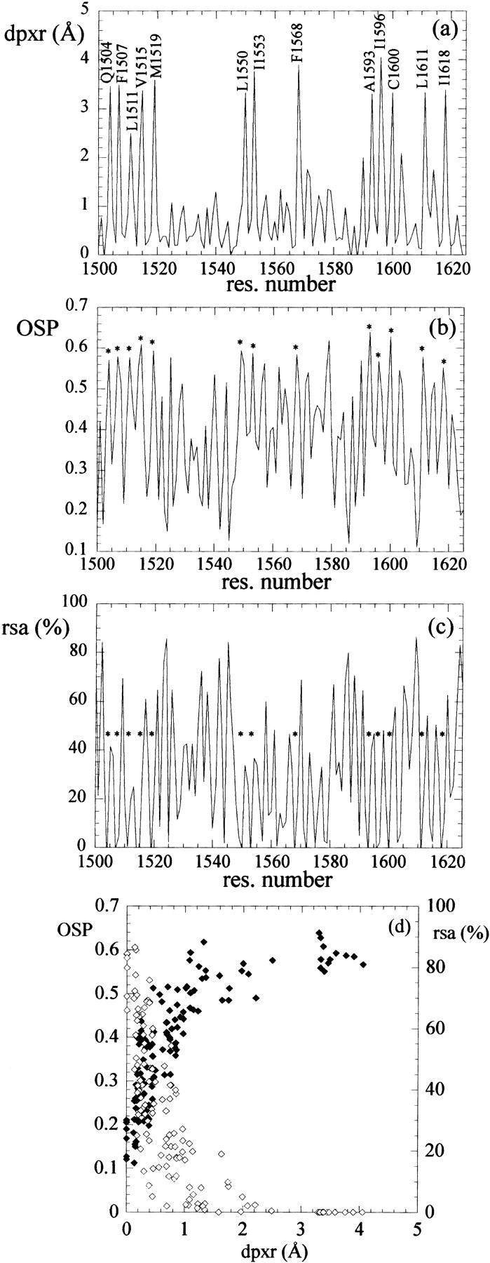
(a) Plot of mean residue dpx (dpxr, Å), (b) occluded surface packing value (OSP), and (c) residue solvent accessibility (rsa, %) versus residue number for the C-terminal bromodomain of human TAFII250 (PDB: 1EQF; residues 1500–1625). In the dpxr plot, important residues are labeled with their amino acid one-letter code and residue number; the same residues are labeled with an asterisk in the OSP and rsa plots. (d) Plot of mean residue dpx (dpxr, Å) versus OSP and rsa (%).

An alternative representation of Fig. 1 a can be obtained plotting the number of observations (%) for each dpx interval. The graphs obtained using intervals of Δ = 1.00, 0.50, 0.25, and 0.10 Å are shown in Fig. 2. Whereas for Δ = 1.00 Å the number of observations is decreasing in a monotone way, at smaller Δ values (Δ = 0.50, 0.25 Å) several maxima appear, the first one corresponding to the surface atoms, the second at dpx ≅ 1.50 Å, the third at dpx ≅ 2.50 Å, and other less pronounced maxima at higher dpx values. For Δ = 0.10 Å, a fine structure for these peaks is appearing.

FIGURE 2.

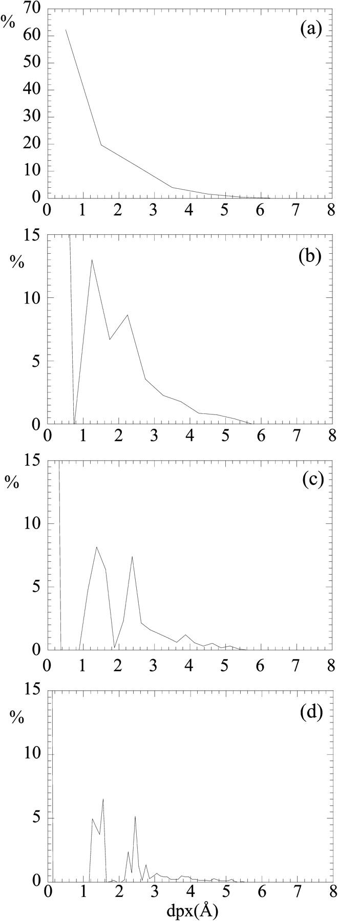
Plot of the number of observations (number of atoms, %) in each dpx interval (a, Δ = 1.00 Å; b, Δ = 0.50 Å; c, Δ = 0.25 Å; d, Δ = 0.10 Å) for the double bromodomain module of human TAFII250 (PDB: 1EQF). In b, c, and d, the peak corresponding to solvent-accessible atoms (dpx = 0) is out of scale for clarity.

For a set of 136 nonhomologous (sequence identity lower than 25%), single-chain protein crystal structures determined at resolution ≤2.0 Å extracted with PDBSELECT (Hobohm and Sander, 1994), we calculated the maximum (dpx_max) and average (dpx_ave) value of dpx for buried atoms in each protein and plotted it as a function of the chain length (Fig. 3). Despite the fact that the data set is highly scattered, especially for chain length > 200, a general trend is observable: the dpx_max increases steeply and linearly in the range 0–100 residues, to flatten beyond 200 residues. A similar behavior is observed for dpx_ave. The highest value observed for dpx_max is ∼8 Å, whereas for dpx_ave it is ∼2.5 Å.

FIGURE 3.

Plot of the maximum (dpx_max, circles) and average (dpx_ave, diamonds) value of dpx versus chain length for a set of 136 single-chain proteins for which the crystal structure has been determined at a resolution ≤2.0 Å.

For the same set of proteins, we calculated the mean residue depth (dpxr) for each of the 20 amino acid types. Taken as a whole, 92% of the residues have at least one solvent exposed atom (dpx = 0), although only 12% have all atoms exposed. The mean value for the 20 amino acid types are in the range 0.45–1.72 Å, with the charged and polar amino acids showing the lowest values, and the aliphatic and aromatic ones showing the highest (Fig. 4, top), in the following order: K < E < D < Q < R < N < P < S < G < T < H < A < Y < C < M < W < L < F < V < I.

FIGURE 4.

Plot of the mean residue depth (dpxr, Å) for each amino acid type (one-letter code), calculated from a set of 136 protein structures (see text for details). Top, overall; bottom, by secondary structure assignment (square, strand; circle; helix; triangle: turn, diamond, coil). Standard deviation values are also shown.

A clear correlation occurs, between mean residue depth and hydrophobicity. The correlation coefficients between dpxr and different hydrophobicity scales are shown in Table 1.

TABLE 1.

Correlation coefficients between different amino acid hydrophobicity scales and mean residue depth

	Depth	K & D*	Chothia†	E & W‡	Janin§	OMH¶	SDH‖
Depth	1
K & D	0.87	1
Chothia	0.86	0.96	1
E & W	0.84	0.88	0.87	1
Janin	0.80	0.86	0.91	0.90	1
OMH	0.90	0.75	0.66	0.72	0.58	1
SDH	0.87	0.73	0.75	0.72	0.81	0.73	1

^*Kyte and Doolittle (1982).

^†Chothia (1976).

^‡Eisenberg et al. (1984).

^§Janin (1979).

^¶Optimized matching hydrophobicity (Sweet and Eisenberg, 1983).

^‖Structure derived hydrophobicity (Casari and Sippl, 1992).

We also calculated the dependence of mean residue depth on secondary structure for the 20 amino acid types in the same set of 136 protein structures. Overall, we found that dpxr values follow the order: dpxr(strand) > dpxr(helix) > dpxr(turn) (Fig. 4, bottom). In most cases the difference in these values is significant, the only exception being T, for which dpxr (strand) ∼ dpxr(helix). Dpxr values for residues classified as coil are somewhat more variable.

The possible correlation between dpx values and fold type was evaluated calculating dpx_max and dpx_ave for the 38 representative domains of the four classes (class 1: mainly α; class 2: mainly β; class 3: mixed α + β; class 4: little secondary structure content) as defined in the CATH database (Orengo et al., 2002), and for representatives of different architectures (A), topologies (T) and homologous superfamilies (H). Large variations in both dpx_max and dpx_ave are observed, also within members with identical topology. For example, for the 17 representative structures of the corresponding homologous superfamilies in the four-helix bundle topology (mainly α, CATH code: 1.20.120) 〈dpx_max〉 = 4.83 Å (standard deviation = 0.92 Å), 〈dpx_ave〉 = 2.02 Å (standard deviation = 0.18 Å). For the 17 representative structures of the corresponding homologous superfamilies in the jelly roll topology (mainly β, CATH code: 2.60.120), which have chain lengths comparable to those of the four-helix bundle group, 〈dpx_max〉 = 5.56 Å (standard deviation = 0.43 Å), 〈dpx_ave〉 = 2.22 Å (standard deviation = 0.14 Å). Results obtained for four-helix bundles and jelly rolls are plotted in Fig. 5.

FIGURE 5.

Plot of the maximum (dpx_max, circles) and average (dpx_ave, squares) values for representative structures of the four-helix bundle topology (a, mainly α-proteins, CATH code: 1.20.120; 17 homologous superfamilies) and the jelly rolls topology (b, mainly β-proteins, CATH code: 2.60.120; 17 homologous superfamilies) plotted versus chain length (number of residues).

As an application of dpx to the identification of possible targets for posttranslational modifications, we selected a set of proteins of known three-dimensional structure, and for which phosphorylation at serine/threonine residues has been reported. In this set, we identified three unrelated proteins for which the target oxydryl is completely buried in the native structure, as calculated by Naccess. These are the elongation factor Tu from Thermus thermophilus (Swiss-Prot: EFTU_THETH, PDB: 1EXM) (Lippmann et al., 1993), hexokinase B from yeast (Swiss-Prot: HXKB_YEAST; PDB: 1IG8) (Heidrich et al., 1997), and bovin rhodopsin (Swiss-Prot: OPSD_BOVIN; PDB: 1HZX) (Brown et al., 1992; Lee et al., 2002). We calculated and extracted dpx values for the OG atom of all Ser/Thr residues in the structures, and sorted them according to their dpx value (Table 2). In all three cases, the OG atom of the phosphorylated residue belongs to the layer of buried atoms that is closest to the surface. The mean residue dpx value can correctly identify the phosphorylated residue as the top ranking in two of the three cases.

TABLE 2.

Dpx values (Å) for the buried (atomic solvent accessibility surface = 0.0 Ų) Ser/Thr oxydryl atoms, layer (L) (L = 0 corresponds to solvent-accessible atoms), residue solvent accessibility (rsa, %), and mean residue dpx (dpxr)

EFTU_THETH, 1EXM
Res.	L	dpx	rsa	dpxr
S309	1	1.42	37.0	0.46
T35	1	1.43	0.4	0.81
T72	1	1.44	6.6	0.41
*T394	1	1.44	2.3	0.81
T188	2	2.43	1.3	1.27
S107	2	2.66	0.0	3.21
S78	2	2.82	0.0	4.44
T116	2	3.08	0.0	3.48
T16	3	4.04	0.0	4.17
T28	3	4.17	0.0	4.56
T32	3	4.56	0.0	4.31
HXKB_YEAST, 1IG8
S396	1	1.41	2.4	0.68
T121	1	1.42	11.2	0.90
S219	1	1.42	4.4	1.86
S293	1	1.42	14.4	0.46
T283	1	1.43	15.5	0.59
T45	1	1.44	1.8	1.28
*S158	1	1.45	35.9	0.24
S306	2	2.38	1.9	1.08
T156	2	2.40	0.4	2.44
T361	2	2.40	0.4	1.12
S385	2	2.52	0.1	1.57
OPSD_BOVIN, 1HZX
S127	1	1.42	1.5	1.78
*S343	1	1.42	13.3	0.48
T193	1	1.43	1.8	0.59
T320	1	1.43	19.5	0.59
T62	2	2.43	2.1	2.34
T251	2	2.43	4.0	1.77
S98	3	3.76	0.8	2.25
T160	3	3.77	0.0	3.52
T94	3	3.82	0.0	3.37
S176	3	4.11	1.5	2.27

The phosphorylated residue in each protein is in bold and labeled by an asterisk. Top ranking numbers are in bold.

To evaluate a possible correlation between residue depth and residue conservation, we selected one of the most common fold type, the Rossman fold, chose one representative structure (PDB: 3CHY), and calculated the sequence entropy S for a structural alignment of 98 structural neighbors on one hand (Mirny and Shakhnovich, 1999), and residue depth (dpxr) and rsa in the reference structure (3CHY) on the other. A plot of dpxr (Å) and rsa (Ų) versus entropy shows that the two distributions are very different (Fig. 6 a). Whereas poorly conserved residues (high entropy) display a wide range of accessible-surface values, highly conserved residues (low entropy) are essentially buried. However, beyond this general observation, rsa provides little or no information on buried residues, as shown by the fact that rsa ∼0 for a whole set of residues displaying a wide range of S (0.1 < S < 0.5). A quantitative correlation between rsa and S for these residues is not applicable. On the contrary, the correlation between dpxr and S can be assumed to be linear (R = 0.80) and maintains its linearity over the entire range of S values, despite the scattering of the data, the deepest residues corresponding to the most conserved ones. This view is confirmed by a plot of dpxr and S versus residue number (Fig. 6 b) where peaks corresponding to deeply buried residues match peaks corresponding to low entropy in a nearly specular fashion. Similar results were obtained for other common fold types, such as the immunoglobulin fold (reference structure: 1TEN) and the TIM barrel fold (reference structure: 2EBN) (data not shown).

FIGURE 6.

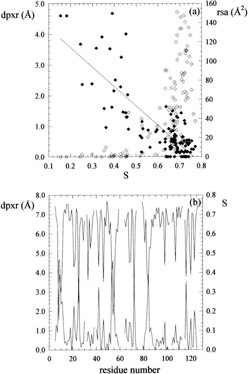
(a) Mean residue depth (dpxr, Å, filled diamonds) and residue-solvent accessibility (rsa, Ų, empty diamonds) calculated for 3CHY and plotted versus sequence entropy (S) calculated for 98 structural neighbors of 3CHY. (b) Mean residue depth (dpxr, Å, lower line) and sequence entropy (S, upper line) plotted versus residue number. In a, also a linear fit of dpxr is shown. In b, line breaks represent positions at which less than two-thirds of residues could be aligned.

DISCUSSION

The dpx value is an atomic property with a simple physical meaning (it is a distance in Å) and it can be thus handled easily: for example, main-chain, side-chain, and residue mean values can be calculated. Fig. 1 shows that mean residue dpx values (dpxr) are very sensitive to structural features. The C-terminal bromodomain of TAFII250 (residues 1500–1625) is made of a four-helix bundle (h1: 1501–1518; h4: 1549–1559; h5: 1564–1584; and h6: 1587–1607) with two additional short helices (h2: 1525–1529; and h3: 1539–1544) and a long C-terminal helix (h7: 1607–1625) (Jacobson et al., 2000). All the residues forming the protein interior can be identified from the plot of the mean residue dpx versus the residue number. For comparison, the OSP value (Pattabiraman et al., 1995) and the residue solvent accessibility are also reported in Fig. 1. Whereas residues contributing to the hydrophobic core, as measured from dpx values, also show high OSP and low accessibility, the dpx parameter is much more sensitive to structural features. It should be remarked, however, that OSP is a measure of packing quality rather than depth, and it applies also to solvent exposed residues. On the contrary, dpx values are related only to the distance of an atom from the surface: they do not take into account contacts with other atoms and cannot be considered a quality index for protein packing. Moreover, DPX provides no information on solvent-exposed atoms, for which dpx = 0. Dpx, OSP, and rsa values can be thus used together to provide complementary information. It is evident from a plot of dpxr values versus either rsa or OSP (Fig. 1, d) or simply the OS (not shown) that residues having zero solvent accessibility can indeed have different depths. In a similar way, residues showing the same OSP (or OS) value can experience very different depths. In other words, atom depth is sensitive where neither solvent accessibility nor the occluded surface can supply an adequate description of the protein interior.

Somewhat different approaches aimed at the calculation of atom depth have been reported. In the “nearest hypothetical water molecule”, the protein is placed in a 3D lattice containing water molecules and the distance between amide N atoms and the nearest hypothetical water molecule is measured. This method was used to correlate this distance to the amide H/D exchange rates, as experimentally determined by NMR (Pedersen et al., 1991). Using a similar approach, Chakravarty and Varadarajan (1999) placed the protein molecule in a water box obtained from a Monte Carlo simulation and calculated the distance of every atom from the nearest water molecule, approximating the dynamics of the protein through sequential rotations and translations, explicitly removing both the water molecules that are found in cavities and those that are found in clefts or surface grooves. In our approach, we took advantage of the rolling sphere algorithm, and reduced the calculation of atom depth to measuring the distance from any protein atom to its nearest solvent-accessible protein neighbor. At the expense of some loss of information for surface atoms (all solvent exposed atoms have dpx = 0 by default), we gained in simplicity, rapidity of execution and flexibility, as the probe radius used by Naccess can be easily varied.

Atom depth is an easily computable quantity, yet it allows one to detect some general features of proteins and protein domains. The first one is a multiple layer organization of protein atoms, as derived from a plot of the number of observations (%) for each dpx interval (Fig. 2). Whereas the majority of the atoms is in the outer, solvent-exposed layer (dpx = 0), the buried atoms are distributed in discrete layers, with a first inner layer with maximum at dpx ≅ 1.50 Å, a second inner layer with maximum at dpx ≅ 2.50 Å, and a set of most deeply buried atoms represented by less well-defined maxima at higher dpx values. The first two inner layers actually correspond to buried atoms that are one or two covalent bonds away from the closest solvent-accessible atom. This multiple layer distribution is not apparent using a Δ value of 1.00 Å (Fig. 2 a) but becomes evident at higher resolution (Δ = 0.50, 0.25, 0.10 Å). Whereas smaller Δ values give a higher resolution, we suggest Δ = 0.50 Å to be a good compromise, as it is closer to the value of a covalent radius, and it can be then connected to a physical meaning. It is remarkable that this type of distribution is peculiar to atom depth, as equivalent plots of atomic-solvent accessibility do not display any layer organization (data not shown).

The second property that is emerging from the analysis of a set of 136 nonhomologous (sequence identity lower than 25%), single-chain protein crystal structures determined at resolution ≤2.0 Å (Fig. 3) is a general limit in the size of proteins and protein domains. The maximum depth of an atom, which can be considered as a measure of the dimension of the protein interior, is increasing steeply in the range 0–100 residues, and flattens for proteins containing more than 200 residues. In other words, the dimension of the buried portion of a protein does not grow indefinitely with chain length, but reaches a maximum depth of ∼8 Å for a chain length of ∼200 residues. A further increase in the dimension may not be beneficial as it would slow down the folding process without any significant increase in the solvent-exposed protein surface, which is most often the functionally “active” part of a biomolecule. At the low end of chain length, the fast increase in the dpx values suggests that a minimal dimension of the hydrophobic core must be reached rapidly to ensure a sufficient stability. Using the average depth of the five deepest atoms in each structure from a set of 65 monomeric proteins, Chakravarty and Varadarajan (1999) obtained results that are similar to ours in the size of the protein at which depth is reaching a plateau (200–250 residues) but different in the depth value obtained (12 Å). This difference can be explained by the fact that the “nearest water molecule” method used by Chakravarty and Varadarajan excludes water molecules placed in clefts and grooves. This is equivalent to having a smoother protein surface, or to using a larger radius for the probe sphere. If we assume that in the first approximation a globular protein can be represented as a sphere, for a 200-residue protein containing ∼1600 nonhydrogen atoms, the expected volume would be ∼32,000 ų, which corresponds to a radius of ∼20 Å. The value found from dpx calculations is much smaller (dpx_max ≈ 6 Å) because the default probe radius of 1.4 Å used in solvent accessibility calculations makes DPX very sensitive to local structural features such as clefts and protruding regions, and this is reflected in the large scatter and small values of dpx (Fig. 3). Indeed, increasing the probe radius to 5.0 Å, local structural features are partially lost, dpx_max values are less scattered, and they reach values of ≈12 Å for ∼200 residue proteins (data not shown), which is in much better agreement with the value expected for a perfect sphere and with that obtained by Chakravarty and Varadarajan (1999). In addition, we should point out that globular proteins are represented better by ellipsoids than by spheres (Taylor et al., 1983). Comparing a sphere with an ellipsoid of identical volume and axis x = y = 0.7 z, the expected dpx_max would further decrease from 12 Å to ∼10 Å.

Similar results in limits in protein and protein domain size were obtained using other independent methods. Xu and Nussinov (1998) constructed an empirical function for the free energy of unfolding versus the chain length and found that the predicted optimal number of residues, which corresponds to the maximum free energy of unfolding, is 100. Fleming and Richards (2000) calculated the OSP using the OS algorithm (Pattabiraman et al., 1995) for a set of 152 single-chain proteins, plotted it versus chain length, and found that it increases markedly up to ∼200 residues, to flatten at larger chain lengths. A recent statistical analysis of domain size in a nonredundant subset of the PDB (Wheelan et al., 2000) showed that the most frequent domain length is ∼100 (Xu and Nussinov, 1998). However, it should be remarked that although results obtained from a statistical analysis of domain size distribution in the PDB structures are in principle dependent on how a domain is defined, results obtained from dpx and OS are not, because no assumption is made a priori. Data obtained from dpx calculations are apparently more scattered than those obtained, for example, using the OSP value (Fleming and Richards, 2000). A possible interpretation is that dpx values are more sensitive to factors different from chain length, like fold type (class, architecture, and topology) (Orengo et al., 2002), secondary structure content, or others.

From the same set of protein structures, we also calculated the mean residue depth for each amino acid type (Fig. 4, top). The charged (K, E, D, R) and carboxylic acid amide (Q, N) amino acids show the lowest dpxr values, whereas the aliphatic (M, L, V, I) and aromatic (W, F) amino acids show the highest. The remaining amino acids (P, S, G, T, H, A, Y, C) show an intermediate character. Interestingly, P, which has an aliphatic and apolar side chain, has a relatively low mean dpxr, whereas H, which is expected to be at least partially charged, has a relatively high mean dpxr value. Overall, these values suggest that mean residue depth can be used as a structure-based hydrophobicity index. Indeed, a good correlation exists between mean residue depth and commonly used hydrophobicity scales (Table 1). It should be pointed out that no assumption is made about the physicochemical properties of each amino acid type in the dpx calculations. In principle, the same approach could be used to derive a mean dpx value for every atom type in a protein.

In addition, we also calculated the dependence of mean residue depth on secondary structure for all amino acid types. A general trend is observable (Fig. 4, bottom): dpxr values for residues in strands are higher than those for residues in helices, with residues in turns showing the lowest dpxr values. This is true also for the statistics run over all residues, and probably reflects the fact that helices are rarely completely embedded in the protein structure, whereas β-strands are often completely buried.

If certain types of protein folds are more compact than others, we might expect different folds to show different dpx_max and dpx_ave values. To verify this hypothesis, we calculated dpx_max and dpx_ave for representative structures of a number of different topologies. As dpx_max and dpx_ave values are strongly dependent on chain length, at least in the range 0–100 residues, we considered proteins within the same size range, and plotted dpx values versus the chain length. As an example, plots for four-helix bundles (CATH code: 1.20.120) and jelly rolls (CATH code: 2.60.120) are shown in Fig. 5. Although a slight increase in dpx_max and dpx_ave is observed, on the average, going from class 1 (mainly α) to class 2 (mainly β) and to class 3 (mixed α + β) (not shown), this variation is smaller than the variations observed within the members of each topology. Calculations carried out on several different protein families (data not shown) confirm this view. We conclude that dpx_max and dpx_ave values for a protein are typical for each single structure, and do not depend strongly on fold type. Indeed, small variations in the shape of the protein interior and conformational modifications at the surface can strongly affect dpx values, especially dpx_max.

Of the several potential applications of dpx, we report here about the identification of “hidden” candidates for posttranslational modifications. As the number of 3D structures is rapidly increasing and the computational tools for the structure-based prediction of posttranslational modifications are becoming more and more sophisticated (Blom et al., 1999), it is relevant to know which atoms should be considered as potential targets and which could be omitted. Intriguingly, we identified three unrelated proteins that are phosphorylated at Ser/Thr residues (Brown et al., 1992; Heidrich et al., 1997; Lee et al., 2002; Lippmann et al., 1993), but for which the solvent-accessible surface of the target oxygen atoms is null. This apparent contradiction is solved by an analysis of dpx values for these atoms. The phosphorylated oxygens, although buried, all show small dpx values and belong to the first inner layer (Table 2). These atoms could then become solvent accessible through internal dynamics movements or small conformational changes, and we thus suggest that they should be taken into account in structure-based predictions of posttranslational modification sites. At the residue level, one might expect low mean residue dpx (dpxr) values for the phosphorylated amino acid. From dpxr values, the target Ser/Thr can actually be identified in two of the three cases, and more reliably than from residue solvent accessibility only (Table 2).

Finally, we analyzed the correlation between residue conservation and residue depth in families of structure-, but not sequence-related, proteins (Mirny and Shakhnovich, 1999). Residue conservation at specified positions within a protein family can arise from different driving factors: thermodynamic stability, folding efficiency, function and binding. Although it can be difficult to isolate the contribution from each of these factors, it has been shown that, to a first approximation, a correlation exists between residue conservation and residue solvent accessibility; in other words, buried residues, which are expected to contribute more to the thermodynamic stability of the protein, are usually more conserved than surface residues (Mirny and Shakhnovich, 1999). This view is reinforced by the correlation found here between residue depth and conservation, measured as sequence entropy. Despite the scattering of the data, the correlation between dpxr and S can be assumed to be linear over the entire range of S values (Fig. 6). More significantly, it maintains its linearity also for residues that are completely or nearly completely buried, in a range where rsa provides little or no information. A simple scenario is hence emerging, where the deeper a residue is buried into the protein structure, the higher its degree of conservation in structurally related proteins.

References

- Blom, N., S. Gammeltoft, and S. Brunak. 1999. Sequence and structure-based prediction of eukaryotic protein phosphorylation sites. J. Mol. Biol. 294:1351–1362. [DOI] [PubMed] [Google Scholar]
- Brown, N. G., C. Fowles, R. Sharma, and M. Akhtar. 1992. Mechanistic studies on rhodopsin kinase. Light-dependent phosphorylation of C-terminal peptides of rhodopsin. Eur. J. Biochem. 208:659–667. [DOI] [PubMed] [Google Scholar]
- Carugo, O., and S. Pongor. 2002. Protein fold similarity estimated by a probabilistic approach based on C(alpha)-C(alpha) distance comparison. J. Mol. Biol. 315:887–898. [DOI] [PubMed] [Google Scholar]
- Casari, G., and M. J. Sippl. 1992. Structure-derived hydrophobic potential. Hydrophobic potential derived from X-ray structures of globular proteins is able to identify native folds. J. Mol. Biol. 224:725–732. [DOI] [PubMed] [Google Scholar]
- Chakravarty, S., and R. Varadarajan. 1999. Residue depth: a novel parameter for the analysis of protein structure and stability. Struct. Fold. Des. 7:723–732. [DOI] [PubMed] [Google Scholar]
- Chothia, C. 1976. The nature of the accessible and buried surfaces in proteins. J. Mol. Biol. 105:1–12. [DOI] [PubMed] [Google Scholar]
- Eisenberg, D., E. Schwarz, M. Komaromy, and R. Wall. 1984. Analysis of membrane and surface protein sequences with the hydrophobic moment plot. J. Mol. Biol. 179:125–142. [DOI] [PubMed] [Google Scholar]
- Fleming, P. J., and F. M. Richards. 2000. Protein packing: dependence on protein size, secondary structure and amino acid composition. J. Mol. Biol. 299:487–498. [DOI] [PubMed] [Google Scholar]
- Heidrich, K., A. Otto, J. Behlke, J. Rush, K. W. Wenzel, and T. Kriegel. 1997. Autophosphorylation-inactivation site of hexokinase 2 in Saccharomyces cerevisiae. Biochemistry. 36:1960–1964. [DOI] [PubMed] [Google Scholar]
- Hobohm, U., and C. Sander. 1994. Enlarged representative set of protein structures. Protein Sci. 3:522–524. [DOI] [PMC free article] [PubMed] [Google Scholar]
- Holm, L., and C. Sander. 1993. Protein structure comparison by alignment of distance matrices. J. Mol. Biol. 233:123–138. [DOI] [PubMed] [Google Scholar]
- Holm, L., and C. Sander. 1996. Mapping the protein universe. Science. 273:595–603. [DOI] [PubMed] [Google Scholar]
- Hubbard, S. J., and J. M. Thornton. 1993. Naccess Version 2.1.1. Department of Biochemistry and Molecular Biology, University College, London.
- Jacobson, R. H., A. G. Ladurner, D. S. King, and R. Tjian. 2000. Structure and function of a human TAFII250 double bromodomain module. Science. 288:1422–1425. [DOI] [PubMed] [Google Scholar]
- Janin, J. 1979. Surface and inside volumes in globular proteins. Nature. 277:491–492. [DOI] [PubMed] [Google Scholar]
- Kabsch, W., and C. Sander. 1983. Dictionary of protein secondary structure: pattern recognition of hydrogen-bonded and geometrical features. Biopolymers. 22:2577–2637. [DOI] [PubMed] [Google Scholar]
- Kyte, J., and R. F. Doolittle. 1982. A simple method for displaying the hydropathic character of a protein. J. Mol. Biol. 157:105–132. [DOI] [PubMed] [Google Scholar]
- Lee, B., and F. M. Richards. 1971. The interpretation of protein structures: estimation of static accessibility. J. Mol. Biol. 55:379–400. [DOI] [PubMed] [Google Scholar]
- Lee, K. A., K. B. Craven, G. A. Niemi, and J. B. Hurley. 2002. Mass spectrometric analysis of the kinetics of in vivo rhodopsin phosphorylation. Protein Sci. 11:862–874. [DOI] [PMC free article] [PubMed] [Google Scholar]
- Lippmann, C., C. Lindschau, E. Vijgenboom, W. Schroder, L. Bosch, and V. A. Erdmann. 1993. Prokaryotic elongation factor Tu is phosphorylated in vivo. J. Biol. Chem. 268:601–607. [PubMed] [Google Scholar]
- Mirny, L. A., and E. I. Shakhnovich. 1999. Universally conserved positions in protein folds: reading evolutionary signals about stability, folding kinetics and function. J. Mol. Biol. 291:177–196. [DOI] [PubMed] [Google Scholar]
- Orengo, C. A., J. E. Bray, D. W. Buchan, A. Harrison, D. Lee, F. M. Pearl, I. Sillitoe, A. E. Todd, and J. M. Thornton. 2002. The CATH protein family database: a resource for structural and functional annotation of genomes. Proteomics. 2:11–21. [PubMed] [Google Scholar]
- Pattabiraman, N., K. B. Ward, and P. J. Fleming. 1995. Occluded molecular surface: analysis of protein packing. J. Mol. Recognit. 8:334–344. [DOI] [PubMed] [Google Scholar]
- Pedersen, T. G., B. W. Sigurskjold, K. V. Andersen, M. Kjaer, F. M. Poulsen, C. M. Dobson, and C. Redfield. 1991. A nuclear magnetic resonance study of the hydrogen-exchange behaviour of lysozyme in crystals and solution. J. Mol. Biol. 218:413–426. [DOI] [PubMed] [Google Scholar]
- Pintar, A., O. Carugo, and S. Pongor. 2002. CX, an algorithm that identifies protruding atoms in proteins. Bioinformatics. 18:980–984. [DOI] [PubMed] [Google Scholar]
- Pintar, A., O. Carugo, and S. Pongor. 2003. DPX: for the analysis of the protein core. Bioinformatics. 19:313–314. [DOI] [PubMed] [Google Scholar]
- Sweet, R. M., and D. Eisenberg. 1983. Correlation of sequence hydrophobicities measures similarity in three- dimensional protein structure. J. Mol. Biol. 171:479–488. [DOI] [PubMed] [Google Scholar]
- Taylor, W. R., J. M. Thornton, and W. G. Turnell. 1983. An ellipsoidal approximation of protein shape. J. Mol. Graph. 1:30–38. [Google Scholar]
- Wheelan, S. J., A. Marchler-Bauer, and S. H. Bryant. 2000. Domain size distributions can predict domain boundaries. Bioinformatics. 16:613–618. [DOI] [PubMed] [Google Scholar]
- Xu, D., and R. Nussinov. 1998. Favorable domain size in proteins. Fold. Des. 3:11–17. [DOI] [PubMed] [Google Scholar]