Collective Chain Dynamics in Lipid Bilayers by Inelastic X-Ray Scattering

Abstract

We investigated the application of inelastic x-ray scattering (IXS) to lipid bilayers. This technique directly measures the dynamic structure factor S(q,ω) which is the space-time Fourier transform of the electron density correlation function of the measured system. For a multiatomic system, the analysis of S(q,ω) is usually complicated. But for multiple bilayers of lipid, S(q,ω) is dominated by chain-chain correlations within individual bilayers. Thus IXS provides a unique probe for the collective dynamics of lipid chains in a bilayer that cannot be obtained by any other method. IXS of dimyristoyl phosphatidylcholine and dimyristoyl phosphatidylcholine + cholesterol at two different concentrations were measured. S(q,ω) was analyzed by three-mode hydrodynamic equations, including a thermal diffusive mode and two propagating acoustic modes. We obtained the dispersion curves for the phonons that represent the collective in-plane excitations of lipid chains. The effect of cholesterol on chain dynamics was detected. Our analysis shows the importance of having a high instrument resolution as well as the requirement of sufficient signal-to-noise ratio to obtain meaningful results from such an IXS experiment. The requirement on signal-to-noise also applies to molecular dynamics simulations.

INTRODUCTION

Recent advances on the technique of inelastic x-ray scattering (IXS) measurement (Sette et al., 1995; Masciovecchio et al., 1996) have improved the energy resolution to the range of meV that allows measurement of collective excitations with energy as low as 0.04 k_BT at room temperature. This technique directly measures the dynamic structure factor, S(q,ω), which is the space-time Fourier transform of the electron density-density correlation function of the measured system. The technique is complementary to the long-existing inelastic neutron scattering (INS) that measures the coherent scattering-length density correlations (Bacon, 1975; Bée, 1988). Two chief advantages of IXS are the wide range of momentum transfer (0.1 nm⁻¹ to 5.0 nm⁻¹) that is not accessible by INS using thermal neutrons, and the requirement of relatively small quantities of sample compared with that for INS.

In this article we report and discuss the collective chain dynamics in lipid bilayers measured by IXS. As it will become clear below, the interpretation of data is complicated for multiatomic systems, but lipid bilayers turn out to be an ideal system for IXS for two reasons. The first reason is that phospholipids in water spontaneously form multilamellae, but there are no correlations between lipid molecules residing in different bilayers. This was rigorously demonstrated first by Smith et al. (1990) on dimyristoyl phosphatidylcholine (DMPC). Let the momentum transfer of x-ray scattering be q. q_z is along the bilayer normal and q_r is the in-plane component. Smith's group measured the diffraction intensities of freely suspended DMPC multilayers around the chain-chain (paraffin) peaks near q_r ∼ 14 nm⁻¹. They found that the q_z-dependence of the chain-chain peaks was that of a single bilayer, containing no interference from neighboring bilayers. Even in the gel phase, the individual chains are positionally uncorrelated from one bilayer to the next. The second reason that lipid bilayers are ideal for IXS studies is that in the same study by Smith's group, it was found that headgroup of the lipid did not contribute to the chain-chain peaks. This means that although the chains of neighboring lipid molecules in the same bilayer were correlated, their headgroups were not. The experiment of Smith et al. (1990) was repeated in our laboratory (Yang et al., unpublished results) with substrate-supported multilayers of various lipids, and the same conclusions were reached. A simple demonstration of the fact that the chains are not correlated between bilayers is the observation that the chain-chain diffraction pattern obtained by in-plane scattering from oriented multilayers (He et al., 1993) is the same as obtained from a powder (i.e., multilayered vesicles) sample. This is an important point because it allows us to measure in-plane chain dynamics using powder samples that are much easier to prepare than a large oriented sample.

Since lipid chains are hydrocarbons and hydrogen has negligible contribution to x-ray diffraction, coherent x-ray scattering in the q-region beyond the lamellar peaks is dominated by carbon-carbon correlations from the lipid chains. In this region of q, IXS measures the dynamic carbon-carbon in-plane correlation functions. From the measured S(q,ω), we will deduce the collective dynamics of lipid chains, including a thermal diffusive mode and propagating acoustic modes. In particular, we will analyze the dispersion curves of the phonons that represent the collective in-plane excitations of lipid chains (a brief report was published in Chen et al., 2001, and Liao and Chen, 2001). Thus IXS provides a unique probe for the collective dynamics of lipid chains in bilayers that cannot be obtained by any other method. DMPC and DMPC + cholesterol at two different concentrations were measured for this experiment. The effect of cholesterol on chain dynamics was observed.

As the synchrotron radiation instrument continues to improve, IXS will undoubtedly become a common technique. One of the strongest incentives for such experiments is that the dynamic range of IXS is comparable to the current molecular dynamics (MD) simulations. IXS is one experiment with which MD can make direct comparison. Indeed MD can also generate S(q,ω) at a comparable quality of the current IXS instruments (Tarek et al., 2001). Thus the analysis presented here is applicable to both IXS and the MD results.

Although the theoretical basis of IXS analysis is quite well-known (Boon and Yip, 1980; Alley and Alder, 1983; de Schepper et al., 1988; Balucani and Zoppi, 1994), we believe it is useful to recapitulate it here at the level of this journal so as to make our results transparent. We found the data analysis for the bilayer experiments highly nontrivial, mainly due to the limitations of the signal-to-noise ratio and the instrumental resolution that could be achieved in practice today. Our analysis points to an important requirement on the instrument resolution and the signal-to-noise ratios. The requirement on the signal-to-noise ratio should also apply to MD simulations.

We believe that the chain dynamics revealed by IXS are closely related to molecular transport across lipid bilayers. It has long been established that the permeabilities of lipid bilayers to various molecules and ions are significant (e.g., Paula et al., 1996; Haines, 2001), yet the cell must maintain molecular gradients across the plasma membrane for its vital functions. Interesting ideas, including MD simulations, have been proposed to relate chain dynamics to permeabilities (Nagle and Scott, 1978; McKinnon et al., 1992; Marrink and Berendsen, 1994; Jansen and Blume, 1995; Paula et al., 1996; Haines, 1994, 2001). Some of these ideas should be correlated with IXS analysis.

In the following, this article will be divided into a brief description of the IXS spectrometer, data collection, theory of collective dynamics, method of data analysis, error treatment, and results and discussion.

EXPERIMENT

A detailed description of the principle and the design of the IXS instrument at the Advanced Photon Source (APS) of Argonne National Laboratory (Argonne, IL) can be found in Sinn et al. (1996) and Sinn (2001). Very briefly, the synchrotron radiation from an undulator is premonochromated by a diamond (1 1 1) double crystal monochromator. The beam then enters a high-resolution in-line monochromator consisting of two nested channel-cut silicon crystals. The first is an asymmetrically cut silicon (4 4 0) crystal. At the second channel cut the beam is reflected twice at an angle 83.2° using the (15 11 3) Bragg reflection of silicon. The beam transmitted through this monochromator has an energy width of 1.3 meV, with a tunable range from 21.50 to 21.70 keV. The beam is focused by a total reflection mirror to 200 μm × 200 μm at the sample. The scattered radiation is collected at 6 m from the sample by a spherically bent matrix of silicon analyzers in a backscattering geometry of Bragg angle 89.98° using the Si (18 6 0) reflection. The radiation is then reflected back into a Cd-Sn-Te detector operating at a low noise level.

The spectrometer works in a reverse mode, which means that the energy of the incident beam is changed while the scattered radiation is being detected at constant energy. The photon flux at the sample was ∼5 × 10⁸ photons/s at a current of 100 mA in the storage ring. The q resolution ± 0.3 nm⁻¹ was determined by the acceptance angle of the analyzer. The spectra were typically taken in the range of ω from −25 meV to +25 meV with a step size of 0.25 meV at a scan rate of 20 s per point. Thus a full energy scan lasted ∼70 min. For each q, 6–8 energy scans were collected and subsequently averaged for analysis. The background signal of the empty sample chamber was also measured and subtracted from the sample data.

The energy resolution of the spectrometer was measured using a Plexiglas cylinder as a sample. Plexiglas acts as a purely elastic scatterer with a negligible width in the elastic peak, thus its spectrum represents the energy resolution function of the instrument. In the case of the IXS spectrometer at the APS, this spectrum can be well-approximated with a mixture of a Gaussian and a Lorentzian lineshape, sometimes called the Pseudo-Voigt function:

(1)

with Γ = 1.90 and η = 0.50. In the following we will call this spectrum R(ω), the instrument resolution function.

1,2-dimyristoyl-sn-glycero-3-phosphocholine (DMPC) was purchased from Avanti Polar Lipids (Alabaster, AL). Cholesterol was purchased from Sigma Chemicals (St. Louis, MO). The hydrated multilamellar lipid samples were made following the protocol given in Olah et al. (1991). Each sample contained ∼50 mg pure lipid. Cholesterol was added at the desired molar ratio to the lipid dissolved in chloroform. The chloroform was blown off under a stream of dry nitrogen and the sample was subsequently dried under vacuum at ∼10 μm Hg for 24 h, to remove all residual solvent. Then 2–3 ml of distilled water was added and the suspension was vortexed vigorously for ∼5 min, and then homogenized using a sonicator for ∼15 min to break up larger aggregates. Afterwards the suspension was quick-frozen using dry ice. The frozen suspension was dried again under vacuum for 24 h. This resulted in a fluffy white powder. The powder samples were then kept at 35°C inside a sealed jar, which had water at the bottom to keep the air inside at 100% relative humidity. The hydration process took 1–2 weeks. The fully hydrated samples had the appearance of a soft transparent gel.

For IXS measurement, the sample was held on a small glass slide put inside a sample chamber with beryllium windows. The sealed chamber contained a small water reservoir to keep the sample fully hydrated during the course of measurement. Its temperature was controlled using a temperature controller (LFI-3500, Wavelength Electronics, Bozeman, MT). The chamber was mounted on a positioning stage to accurately center the sample into the beam. The pathlength through the sample was ∼10 mm, which corresponds approximately to the absorption length of the lipids for the x-ray energy (21.657 KeV) used.

THEORY FOR IXS OF LIPID BILAYERS

We start with the general differential cross section for IXS (Heitler, 1954) which is similar to the neutron cross section for INS (Marshall and Lovesey, 1971),

(2)

where r_o is the classical radius of electron, and are, respectively, the momentum, energy, and polarization of the incident and the scattered photon, (q,ω) are defined as , and r_ℓ(t) is the position of the ℓ^th electron at time t. The bracket 〈 〉 implies a thermal ensemble average. The sum over electrons labeled by ℓ can be written as a sum over atoms labeled by α by introducing the atomic form factor f_α(q):

As explained in the Introduction, we anticipate the coherent scattering being dominated by the carbon atoms of the lipid chains. Let f_c(q) be the atomic form factor of carbon and N the total number of carbon atoms in the sample. We define the dynamic structure factor, S(q,ω), by

(3)

(4)

where is the number density of carbon atoms at position r and time t. We propose that the dynamics governing can be described by hydrodynamic equations generalized to large values of q (Boon and Yip, 1980; Alley and Alder, 1983; de Schepper et al., 1988; Balucani and Zoppi, 1994). We understand that it is commonly stated that hydrodynamics is, strictly speaking, valid only in the limit , where σ is the particle size. However, it has been argued (Boon and Yip, 1980; Balucani and Zoppi, 1994) that the actual domain of validity is determined not by the particle size but by the requirement that the explored length scale must comprise a sufficiently large number of collision events. Thus the restrictive condition should be qℓ ≪ 1, where ℓ is the mean free path, rather than qσ ≪ 1. In fluids, ℓ is considerably smaller than σ, so the hydrodynamic description can be extended to q-values much higher than what is expected from intuitive considerations. The validity of generalized hydrodynamics has been demonstrated by the simulation results of hard spheres (Alley and Alder, 1983) and Lennard-Jones fluid (de Schepper et al., 1988).

For the sake of clarity, we briefly recapitulate the basis of the generalized hydrodynamic equations. This is most comprehensible by considering first the case of no energy dissipation. We will consistently keep only the linear terms and start with three equations: Eq. 5.1, the equation of continuity,

(5.1)

Eq. 5.2, the divergence of the Euler equation (or the Navier-Stokes equation without viscosity),

(5.2)

and Eq. 5.3, the thermodynamic relation (per carbon atom),

(5.3)

In these equations, m is the effective mass of each carbon atom, is the momentum density, p the pressure, s the entropy, and T the temperature. In the absence of dissipation, ds is zero. If we expand dp in Eq. 5.2 by , we now have three equations in three variables, i.e., n, , and T.

We define the thermal energy per unit volume as and transform the three equations to the q-space: , , and , where j is the longitudinal component of momentum, flux J. We then introduce the normalized variables: , , and . The normalization factors are given as follows.

(6)

where the static structure factor S(q) satisfies the important relation

(7)

From the definition of J(r,t), one has, by the equipartition principle,

(8)

Similarly, we have (Landau and Lifshitz, 1969)

(9)

with

The three equations (Eqs. 5.1–5.3) become

(10.1)

(10.2)

(10.3)

These equations are no different from the standard hydrodynamic equations without dissipation (Landau and Lifshitz, 1959), except the variables are normalized. The extension to high q-region requires some of the thermodynamic coefficients to have a nonlocal behavior. For example, a local free energy expansion (Landau and Lifshitz, 1969) becomes

(11)

In the q-space, Therefore, the thermodynamic coefficient becomes q-dependent and is related to S(q) by

(12)

With the relation in Eq. 12, Eqs. 10.1–10.3 can be written in a symmetric form

(13)

where

(14)

and similarly we extend to a q-dependent quantity

(15)

The most important point of Eq. 13 is the symmetry of the matrix that leaves only two parameters in the nondissipative hydrodynamic equations. To complete the generalized hydrodynamic equations, we must include a viscosity term in Eq. 5.2 to make it the Navier-Stokes equation (Landau and Lifshitz, 1969), and include a dissipative term in Eq. 5.3 so ds/dt is positive (Landau and Lifshitz, 1959). The dissipative coefficients are also assumed to be q-dependent:

(16)

This set of three-mode hydrodynamic equations will be used to analyze the IXS data from lipid bilayers. The results will be expressed in four function parameters, f_un(q), f_uT(q), z_u(q), and z_T(q).

METHOD OF DATA ANALYSIS

The connection between the hydrodynamic equations and the IXS measurement is given by

(17)

which is evident from Eqs. 4 and 6. The Fourier transform on the right-hand side of Eq. 17 can be solved from Eq. 16, so that S(q,ω)/S(q) is a function of the quantities in the matrix of Eq. 16. If one defines , it is straightforward to show

(18)

The second equation of Eq. 18 is the solution of Eq. 16. This solution can be expressed in the form of hydrodynamic modes:

(19)

expressing the shape of the measured S(q,ω) as a sum of three Lorentzians centered at ω = 0, ± ω_s. This is essentially a Rayleigh-Brillouin triplet as seen in light scattering (Landau and Lifshitz, 1969), which attributes the width of the central peak Γ_h to the heat diffusion damping, and the inelastic side peaks to the sound frequency ω_s and damping γ_s. The Lorentzian parameters, Γ_h, ω_s, and γ_s, in Eq. 19 are functions of the four fitting parameters given in Eqs. 16 and 18. In fact, the number of fitting parameters can be further reduced, if the static structure factor, S(q), is measured independently and is used to predetermine f_un according to Eq. 14. In that case, the three-mode hydrodynamic theory has only three free parameters. Alternatively, Eq. 14 can be used as a check of self-consistency for a four-parameter fit. The latter approach was taken in the present analysis.

A representative data spectrum S(q,ω)/S(q) is shown in Fig. 1, where the measured S(q,ω) was normalized by adjusting the amplitude such that the integration over ω is equal to ‘1’ (see Eq. 7). The spectrum is dominated by the elastic line at ω = 0 where the spectrum is barely wider than the instrument resolution. Important signals are contained in the side wings, which are two orders-of-magnitude smaller than the central peak. A weighted least-square fit to the data was calculated according to Eq. 18, using a downhill gradient search (Press et al., 1992) to minimize the χ² function defined as in the four-dimensional parameter (f_un, f_uT, z_u, and z_T) space, where y_i is the data point, f(x_i) the calculated value for the fit, and w_i the statistical weight of the point i. The number N stands for the degrees of freedom, i.e., the number of the data points minus the number of parameters. For each value of q, the calculated dynamic structure factor, Eq. 18, was multiplied by a Boltzmann term corresponding to the temperature used in the experiment, so as to satisfy the quantum mechanical detailed balancing condition (Bée, 1988). The model equation for the least-square fitting was obtained by the convolution of the resolution function, R(ω), of Eq. 1, and the normalized theoretical structure factor denoted as :

(20)

FIGURE 1.

IXS spectrum of pure DMPC at T = 290 K and q = 7.5 nm⁻¹. The continuous line depicts the instrumental resolution function of the spectrometer, fitted by Eq. 1 with Γ = 1.90, η = 0.50. The spectrum is dominated by the elastic line at ω = 0. The inset shows the same plot with the y-axis enlarged by a factor of 10. The intensity of the side-peaks is roughly two orders-of-magnitude smaller than the central peak.

The dominance of the central peak over the side wings, as shown in Fig. 1, presents a problem for the χ² fitting. In the least-square fit, the data points are usually weighted according to their statistical errors. Using Poisson statistics for the photon counts, this implies that the dominant central peak will have the largest relative weight in the fit and its importance will dominate the wings, that is, the deviations of the model from the data in the central peak region will be more important in the χ² than those in the wings. However, as the central peak of the theoretical model (S_theo in Eq. 20) is extremely narrow, the width of the measured S(q,ω) in the central region (∼ω = 0) is dominated by the instrument resolution. With the large statistical weight for this peak, the fit algorithm tends to adjust the fit parameters for inaccuracies in the resolution function while allowing a decrease in the fit quality for the less weighted side wings. These wings, on the other hand, are less sensitive to the exact shape of the resolution function R(w), since their widths are much larger, and thus the model parameters are more directly expressed there. To better determine the model parameters, we somewhat arbitrarily decreased the statistical weight given to the central peak; for example, reducing the weight of five data points ∼ω = 0, each by a factor of 10. This did not alter the results of the fit to the spectra of the three lowest q-values (see below).

ERROR TREATMENT

To extract an error estimate of the fitted parameters from a weighted least-square fit, one usually uses the curvature matrix of the χ² function at the minimum (Press et al., 1992). An error propagation could then be used to find the error bars for the physical parameters Γ_h, γ_s, and ω_s. This procedure is however cumbersome and not trustworthy in a four-dimensional parameter space where there are numerous local minima. Therefore, we use a different method to estimate the error by direct numerical trials. We first produced three model data sets with assumed parameters that have the same energy resolution and step size as the spectra recorded in the experiment. The data sets are exemplary of three different experimental situations encountered as shown in Fig. 2: Model A has well-separated side peaks; in Model B the side peaks are ∼3 meV from the central peak; and in Model C the side peaks are within the instrumental resolution (∼1.8 meV) of the central peak. Then we used the least-squares fitting algorithm described above to find the best values for the fitting parameters. The results are listed in Table 1 in the column labeled fit 1. For all three models the fitted values coincide with the true values rather well, and we took this as a proof for the correctness of the implemented algorithm. (To exclude the possibility of a circular argument, the model data sets were produced by an independent algorithm. The fitting algorithm was written in the ‘C’ programming language, whereas the model data sets were produced using the Mathematica program.) The observed deviations from the exact values are the results of truncation errors in the calculation of the convolution. Next, to simulate the real experimental data, we added random noise to the model data sets comparable to the statistical errors encountered in the experiment. Two noise levels corresponding to 15,000 counts/s (fit 2) and 5000 counts/s (fit 3) at the elastic peak were added, and subsequently fitted. The results are listed in Table 1.

FIGURE 2.

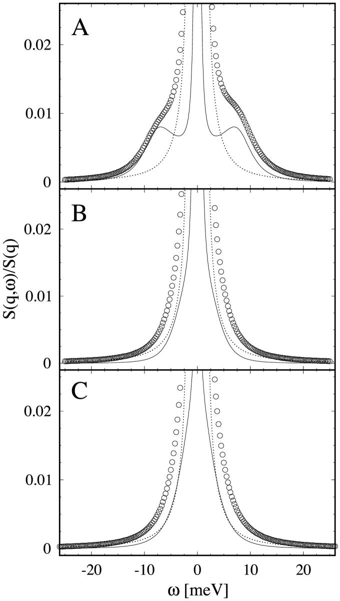
The three model data sets used to test the consistency and accuracy of the data analysis (see text). A theoretical S(q,ω) (thin solid line) was created by assuming values for the fitting parameters, and then was convoluted with the resolution function (dotted line) to produce the model data (circles) for the fitting test. Model A has well-separated side peaks. Model B has side peaks at ∼3 meV from the central peak. Model C has side peaks within ∼2 meV of the central peak. The fits to these model data sets were referred to as fit 1 in text. For fit 2 and fit 3, noises comparable to the real data were added to the model data.

TABLE 1.

	Model A				Model B				Model C
	Exact	Fit 1	Fit 2	Fit 3	Exact	Fit 1	Fit 2	Fit 3	Exact	Fit 1	Fit 2	Fit 3
fun	3.43	3.44	3.40	3.45	1.60	1.61	1.60	1.50	2.15	2.14	2.09	2.13
fuT	8.02	8.02	7.96	8.03	4.04	4.02	4.22	4.21	4.44	4.48	4.47	4.58
zu	7.12	7.20	6.95	6.97	6.44	6.50	6.22	4.90	9.80	9.93	9.41	9.61
zT	0.33	0.32	0.37	0.37	0.71	0.70	0.93	1.08	0.05	0.10	0.12	0.19
	Calculated Lorentzian parameters
Γh	0.05	0.05	0.05	0.06	0.08	0.08	0.09	0.10	0.01	0.02	0.02	0.03
γs	3.70	3.73	3.63	3.64	3.54	3.56	3.53	2.94	4.92	5.00	4.76	4.88
ωs	8.02	8.01	8.01	8.08	3.22	3.17	3.61	4.01	0.72	0.67	1.63	1.78

In Model A, where the side peaks are well-separated from the central line, all four fitting parameters were reproduced correctly, even at high noise levels. The deviations are less than 2.5%. In Model B, where the side peaks are ∼3 meV away from the central line, the errors in all three Lorentzian parameters increased in comparison to Model A. At low noise level the deviation for the width and position of the side peaks is roughly 10%, but it increased to ∼25% for the high noise level. In the case of Model C, where the side peaks are close to ω = 0, the results show that the determination of the parameters is rather unreliable. Primarily, we found that varying the initial parameter values could be very hazardous and often caused the fit to end in a completely different minimum of χ². Even at the low noise level (fit 2), the fitted ω_s is more than twice the true position. This is partly a problem of the instrument resolution. It can be shown by the same method that a higher instrument resolution would solve this problem. Another way to remedy the problem of Model C is to increase the measurement time to reduce the statistical errors. This is impractical, however, as the error would need to be improved by ∼2 orders of magnitude, which would require an enormous measurement time.

RESULTS AND DISCUSSION

For each sample, the static structure factor S(q) was measured first (Fig. 3). Since our samples were not oriented, lamellar peaks appeared in the low q region. However, for q > 4.5 nm⁻¹, the measured S(q) is essentially the same as the in-plane S(q) measured from an oriented multilayer sample with q oriented in-plane (Weiss and Huang, unpublished results; the in-plane S(q) of DLPC was shown in He et al., 1993, which is similar to DMPC). The peak at ∼14.5 nm⁻¹ is the well-known paraffin peak originated from chain-chain correlations (Warren, 1933). As stated in the Introduction, this is an indication that for q > 4.5 nm⁻¹ the coherent scattering is dominated by chain-chain correlations within individual bilayers.

FIGURE 3.

Static structural factor S(q) of pure DMPC in the fluid phase (T = 308 K, solid line) and in the gel phase (T = 294 K, dotted line). The lamellar peaks in the low q-region indicate the powder character of the sample. The peaks ∼14.0 nm⁻¹ are caused by chain-chain correlations in the core of the lipid bilayer. The chains are all trans (ordered) in the gel phase, but gauche rotamers are excited (thus disordered) in the fluid phase. This can be seen in the broadening of the peak and its slight shift to lower q-values as the temperature increased. One of the fitting parameters, f_un(q), was compared with the measured as a check of self-consistency (see Eq. 14).

About 10 IXS spectra were measured for each sample, with q-values ranging from 4.5 to 20 nm⁻¹. The data were analyzed as described above. Least-squares fits were started with several different initial values for the fitting parameters (f_un, f_uT, z_u, and z_T), and the iterations were stopped after a reasonable convergence toward a small χ² was reached. In the event that different minima were reached for the same data set, the fit with the lowest χ² was used. Subsequently the fitting parameters were used to calculate the Lorentzian parameters Γ_h, ω_s, and γ_s. For all the samples, the spectra of the lowest four q-values were fitted well with a final χ² value being less than 2 (Fig. 4). The spectra of q > 10 nm⁻¹ are of the type of Model C discussed in the last section, for which we could not obtain reliable fits. However, we have no doubt that since the IXS instruments continue to improve, we will be able to obtain analyzable lipid data at the high q-region in the near future.

FIGURE 4.

Normalized S(q,ω), or S(q,ω)/S(q), for pure DMPC in the gel phase (T = 290 K, top row) and fluid phase (T = 308 K, bottom row) at the q-values indicated. The graphs show the measured data (circles; for clarity only every other data point is depicted) together with the fitted model function (thick solid line). Also shown are the instrumental resolution (dotted line) and the fitted model function before convolution (thin solid line).

The low q-spectra show how useful information is obtained from IXS. The properties of chain dynamics are expressed in the quantities Γ_h, ω_s, and γ_s. It is well-known that in the hydrodynamic limit of q → 0, the peak widths Γ_h and γ_s are proportional to q², whereas the sound energy, ω_s, is proportional to q (Landau and Lifshitz, 1959). However, these q-dependences change as q increases. We learned this from the MD simulations of hard-sphere fluids (Alley and Alder, 1983; Cohen et al., 1984) and Lennard-Jones fluids (De Schepper et al., 1984a, 1988) as well as from the inelastic neutron scattering of real fluids (De Schepper et al., 1983, 1984b; Van Well and de Graaf, 1985; Bodensteiner et al., 1992). The heat (Rayleigh) mode is the mode of lowest energy. In the q-range of our interest, its width Γ_h is inversely proportional to the static structure factor S(q) (Cohen et al., 1987), thus its value first increases by its q² dependence, but then decreases to a minimum as S(q) reaches its maximum—often called the de Gennes narrowing (De Gennes, 1959). The latter occurs at q = q_G ∼ 14.5 nm⁻¹ corresponding to the size of the chain cross section 2π/14.5 ∼ 0.43 nm. At this and larger values of q, all local conservation laws expressed in terms of molecular densities disappear, except for the conservation of mass. Thus, near q = q_G, the heat mode is expected to coincide with the self-diffusion mode of the chains.

The extended sound (Brillouin) mode gives two parameters, ω_s and γ_s. As we see in Fig. 4, the sound peaks do not always appear as separate maxima. They might overlap with the central Rayleigh peak. For liquid argon and neon (De Schepper et al., 1983; Van Well and de Graaf, 1985), and high-density hard-sphere or Lennard-Jones fluids (Cohen et al., 1984), the dispersion curves show a propagation gap for a certain range of q, where ω_s = 0 and the modes do not propagate. In such a region there are two purely damped modes. The location of this region is q∼q_G. For liquid cesium near its melting point (Bodensteiner et al., 1992) and low-density hard-sphere fluids, the dispersion curves show a minimum, rather than a gap, also at q = q_G. Physically, a gap or a dip in ω_s versus q can be understood as caused by the competition between the elastic (restoring) force and the dissipative process, which for small q, are proportional to q and q², respectively. Thus in the hydrodynamic (small q-) region, the elastic force prevails and the sound propagates. For larger q, however, the dissipative force may become comparable to or dominating over the elastic force, so that sound barely propagates or no propagation is possible. For still larger q-values, the molecules behave like an ideal gas (De Gennes, 1959), thus the propagating mode appears again, according to the study on hard-sphere fluids (Cohen et al., 1984).

The pure DMPC sample was measured at two different temperatures, T = 290 K and T = 308 K, corresponding to the gel (L_β′) phase and the fluid (L_α) phase of the lipid, respectively. The data and the final fit function for S(q,ω)/S(q) are shown in Fig. 4. All spectra in this q-range were fitted quite well. The q-dependence of the fitting parameter f_un(q) agrees with the measured as a check of self-consistency (Eq. 14).

In the gel phase the sound modes are most clearly distinguishable. They appear in the raw data as pronounced shoulders to the dominant central peak. Each final theoretical fit function (before the convolution with the instrument resolution) consists of a central (or Rayleigh) peak and two side peaks shifting in frequency with q that correspond to the Stokes and anti-Stokes components of the Brillouin doublet. The dispersion relation for the sound mode ω_s versus q is shown in Fig. 5, and the width of the Brillouin peak γ_s in Fig. 6. We stress that these were modes of sound propagating in the plane of individual bilayers. At the lowest measurable point in q (∼4.5 nm⁻¹), the sound frequency is ∼7 meV, and width γ_s ∼ 2.5 meV. With increasing q, the sound frequency first increases to ∼8.5 meV at q ∼ 7.5 nm⁻¹, and then decreases. In the meantime, the width steadily increases with q. At q = 10 nm⁻¹, the width becomes comparable to the frequency. The spectra beyond q = 10 nm⁻¹ could not be analyzed reliably as explained in the last section. The same general behavior can be seen in the fluid phase of DMPC, although the Brillouin peaks are less obvious. The reason is that the sound frequencies are lower than the gel phase whereas the peak widths are larger (see Figs. 5 and 6). On the other hand, the measured width of the heat mode Γ_h (Fig. 6) did not show any systematic behavior, indicating large uncertainties. Of the three Lorentzian parameters, this is the least accurate because the central peaks were barely larger than the instrumental resolution (Figs. 1 and 4).

FIGURE 5.

Dispersion curves of the sound mode excitations for the four lipid samples measured. The lines are drawn as a guide for the eye. The initial slope of the dispersion gives the high-frequency sound speed, which is indicated for the pure DMPC in the gel phase (2340 m/s, dotted line) and in the fluid phase (1420 m/s, dash-dotted line).

FIGURE 6.

The widths of the Brillouin peak, Γ_h, and the Rayleigh peak, γ_s, as determined by Eq. 19. The symbols are the same as in Fig. 5. The lines in the figure for γ_s are drawn as a guide for the eye.

Although the small q-region was not accessible by this technique, each dispersion curve is apparently a monotonically increasing function of q in the small q-region until it reaches a maximum at q ∼ 7.5 nm⁻¹, then decreases. As mentioned above, this is the general feature of high-frequency sounds in liquids, as seen by inelastic neutron scattering of liquid argon (De Schepper et al., 1983), neon (Van Well and de Graaf, 1985), and cesium (Bodensteiner et al., 1992). A rough estimate of adiabatic sound velocity was obtained by the initial slope to the dispersion curve: 2340 m/s for pure DMPC in the gel phase and 1420 m/s in the fluid phase. These values are considerably smaller than the high-frequency sound velocities of water measured by the same technique (Sette et al., 1995; Liao et al., 2000).

Two samples of DMPC with cholesterol at 40 mol % and 20 mol % were measured at T = 308 K, the same temperature at which the fluid phase DMPC was measured. As shown in Figs. 5 and 6, their dispersion curves and damping width γ_s fall in between the gel phase and the fluid phase of pure DMPC. The in-plane sound velocities were calculated to be ∼1730 m/s for DMPC with 40 mol % cholesterol and 1540 m/s for DMPC with 20 mol % cholesterol. The effect of cholesterol on the properties of phospholipid bilayers is one of the most studied membrane problems (see review in Gennis, 1989). X-ray and neutron diffraction show that cholesterol inserts normal to the bilayer with the –OH group located near the ester carbonyl of the lipid (Worcester and Franks, 1976). Infrared spectroscopic experiments showed that above the main (gel-fluid) transition, cholesterol decreases the fraction of the gauche rotamers in the lipid chains, whereas below the transition the effect is opposite (Cortijo et al., 1982). The result is that lipid-cholesterol mixtures behave roughly as intermediate between the gel and fluid states of pure phospholipids. Our result here shows that this is also true for the collective chain dynamics. This might be connected to the ability of cholesterol to reduce ion leakage across the membrane (Haines, 2001) as the collective modes have previously suggested to play a role in the transport of small molecules and ions across the membrane (Paula et al., 1996).

The work presented above demonstrates that IXS provides a unique probe for high-frequency (∼10¹² s⁻¹) collective in-plane chain dynamics. It is highly desirable to measure Γ_h, ω_s, and γ_s accurately and up to q ∼ 15 nm⁻¹. As was found in hard-sphere fluids (Cohen et al., 1984), the high q-region is rich in dynamics information. It would be interesting to see whether the collective dynamics of lipid bilayers are similar or significantly different from ordinary fluids. One of the outstanding membrane problems has been: which property of lipid bilayer is directly related to transbilayer molecular permeability? Since the original solubility-diffusion theory (Findelstein, 1976) was found to deviate from experiments (Deamer and Bramhall, 1986), it has been argued that some features of lateral chain motion are responsible for the molecular transport across the bilayer, such as transient defects, transient pores, or gauche-trans-gauche kinks (Nagle and Scott, 1978; Deamer and Bramhall, 1986; Paula et al., 1996; Haines, 1994; 2001). Essentially the lipid chains must separate just enough at some discrete frequency to allow molecules to pass through the membrane (Haines, 1994). But it has been difficult to relate these theoretical ideas to experiment. We suggest a combination of collective chain dynamics by IXS, MD, and permeability measurements to gain insight into the permeability problem that has recently gained importance in applications to drug delivery.

As noted in the Introduction, this frequency domain is ideal for MD simulations. Indeed we would like to stress that the measurement of IXS provides the most direct comparisons with MD, because both techniques probe the same frequency domain. Our IXS experiment performed at the APS revealed an important criterion for data analysis. At the resolution of the current instrument and at the currently achievable photons statistics, only the spectra <q ∼ 10 nm⁻¹ were analyzable. The dispersion curves indicate a low-energy region (soft modes) >q ∼ 10 nm⁻¹ (Chen et al., 2001; Liao and Chen, 2001) that could be important because they would be the prevalent modes of chain excitations. To measure this region, both the instrument resolution and photon statistics need to be improved. Obviously a similar criterion applies to the simulated S(q,ω) produced by MD.

References

- Alley, W. E., and B. J. Alder. 1983. Generalized transport coefficients for hard spheres. Phys. Rev. A27:3158–3173. [Google Scholar]
- Bacon, G. E. 1975. Neutron Diffraction. Clarendon Press, Oxford. pp. 283–322.
- Balucani, U., and M. Zoppi. 1994. Dynamics of the Liquid State. Clarendon Press, Oxford. pp. 216–266.
- Bée, M. 1988. Quasielastic Neutron Scattering. Adam Hilger, Bristol. pp.11–71.
- Boon, J. P., and S. Yip. 1980. Molecular Hydrodynamics. Dover Publications, New York. pp. 237–278.
- Bodensteiner, T., C. Morkel, and W. Glaser. 1992. Collective dynamics in liquid cesium near the melting point. Phys. Rev. A. 45:5709–5720. [DOI] [PubMed] [Google Scholar]
- Chen, S. H., C. Y. Liao, H. W. Huang, T. M. Weiss, M. C. Bellisent-Funel, and F. Sette. 2001. The collective dynamics in fully hydrated phospholipid bilayers studied by inelastic x-ray scattering. Phys. Rev. Lett. 86:740–743. [DOI] [PubMed] [Google Scholar]
- Cohen, E. G. D., I. M. de Schepper, and M. J. Zuilhof. 1984. Kinetic theory of the eigenmodes of classical fluids and neutron scattering. Physica. 127B:282–291. [Google Scholar]
- Cohen, E. G. D., P. Westerhuijs, and I. M. de Schepper. 1987. Half-width of neutron spectra. Phys. Rev. Lett. 59:2872–2874. [DOI] [PubMed] [Google Scholar]
- Cortijo, M., A. J. Alonzo, J. C. Gomez-Fernandez, and D. Chapman. 1982. Intrinsic protein-lipid interactions: infrared spectroscopic studies of gramicidin A, bacteriorhodopsin, and Ca2+-ATPase in biomembranes and reconstituted systems. J. Mol. Biol. 157:597–618. [DOI] [PubMed] [Google Scholar]
- De Gennes, P. G. 1959. Liquid dynamics and inelastic scattering of neutrons. Physica. 25:825–839. [Google Scholar]
- De Schepper, I. M., P. Verkerk, A. A. van Well, and L. A. Graaf. 1983. Short-wavelength sound modes in liquid argon. Phys. Rev. Lett. 50:974–977. [Google Scholar]
- De Schepper, I. M., J. C. van Rijs, A. A. van Well, P. Verkerk, and L. A. de Graaf. 1984a. Microscopic sound waves in dense Lennard-Jones fluids. Phys. Rev. A29:1602–1605. [Google Scholar]
- De Schepper, I. M., P. Verkerk, A. A. van Well, and L. A. de Graaf. 1984b. Non-analytic dispersion relations in liquid argon. Phys. Lett. 104A:29–32. [Google Scholar]
- De Schepper, I. M., E. G. D. Cohen, C. Bruin, J. C. van Rijs, W. Montfrooij, and L. A. de Graaf. 1988. Hydrodynamic time correlation functions for a Lennard-Jones fluid. Phys. Rev. A38:271–287. [DOI] [PubMed] [Google Scholar]
- Deamer, D. W., and J. Bramhall. 1986. Permeability of lipid bilayers to water and ion solutes. Chem. Phys. Lipids. 40:167–188. [DOI] [PubMed] [Google Scholar]
- Findelstein, A. 1976. Water and nonelectrolyte permeability of lipid bilayer membrane. J. Gen. Physiol. 68:127–135. [DOI] [PMC free article] [PubMed] [Google Scholar]
- Gennis, R. B. 1989. Biomembranes. Springer-Verlag, New York. pp. 73–74.
- Haines, T. H. 1994. Water transport across biological membranes. FEBS Lett. 346:115–122. [DOI] [PubMed] [Google Scholar]
- Haines, T. 2001. Do sterols reduce proton and sodium leaks through lipid bilayers? Progr. Lipid Res. 40:229–324. [DOI] [PubMed] [Google Scholar]
- He, K., S. J. Ludtke, Y. Wu, and H. W. Huang. 1993. X-ray scattering with momentum transfer in the plane of membrane: application to gramicidin organization. Biophys. J. 64:157–162. [DOI] [PMC free article] [PubMed] [Google Scholar]
- Heitler, W. 1954. The Quantum Theory of Radiation. Dover, New York. pp. 189–196.
- Jansen, M., and A. Blume. 1995. A comparative study of diffusive and osmotic water permeation across bilayers composed of phospholipids with different head groups and fatty acyl chains. Biophys. J. 68:997–1008. [DOI] [PMC free article] [PubMed] [Google Scholar]
- Landau, L. D., and E. M. Lifshitz. 1969. Statistical Physics. Addison-Wesley, Reading, MA. pp. 348–354, 362–387.
- Landau, L. D., and E. M. Lifshitz. 1959. Fluid Mechanics. Pergamon Press, New York. pp. 1–50.
- Liao, C. Y., S. H. Chen, and F. Sette. 2000. Analysis of inelastic x-ray scattering spectra of low-temperature water. Phys. Rev. E61:1518–1526. [DOI] [PubMed] [Google Scholar]
- Liao, C. Y., and S. H. Chen. 2001. Theory of the generalized dynamic structure factor of polyatomic molecular fluids measured by inelastic x-ray scattering. Phys. Rev. E 64:021205.1–10. [DOI] [PubMed] [Google Scholar]
- Marrink, S.-J., and H. J. C. Berendsen. 1994. Simulations of water through a lipid bilayer. J. Phys. Chem. 98:4155–4168. [Google Scholar]
- Marshall, W., and S. W. Lovesey. 1971. Theory of Thermal Neutron Scattering. Clarendon Press, Oxford. pp. 1–40.
- Masciovecchio, C., U. Bergmann, M. Krisch, G. Ruocco, F. Sette, and R. Verbeni. 1996. A perfect crystal x-ray analyzer with meV energy resolution. Nucl. Instr. Meth. Phys. Res. B. 111:181–188. [Google Scholar]
- McKinnon, S. J., S. L. Whittenburg, and B. Brooks. 1992. Nonequilibrium molecular dynamics simulation of oxygen diffusion through hexadecane monolayers with varying concentrations of cholesterol. J. Phys. Chem. 96:10497–10506. [Google Scholar]
- Nagle, J. F., and H. L. Scott. 1978. Lateral compressibility of lipid mono- and bilayers theory of membrane permeability. Biochim. Biophys. Acta. 513:236–243. [DOI] [PubMed] [Google Scholar]
- Olah, G. A., H. W. Huang, W. Liu, and Y. Wu. 1991. Location of ion binding sites in the gramicidin channel by x-ray diffraction. J. Mol. Biol. 218:847–858. [DOI] [PubMed] [Google Scholar]
- Paula, S., A. Volkov, A. Van Hoek, T. Haines, and D. Deamer. 1996. Permeation of protons, potassium ions and small polar molecules through phospholipid bilayers as a function of membrane thickness. Biophys. J. 70:1061–1070. [DOI] [PMC free article] [PubMed] [Google Scholar]
- Press, W., S. Teukolsky, W. Vetterling, and B. Flannery. 1992. Numerical Recipes in C. Cambridge University Press, Cambridge, UK. pp. 681–190.
- Sette, F., G. Ruocco, M. Krisch, U. Bergmann, C. Masciovecchio, V. Mazzacurati, G. Signorelli, and R. Verbeni. 1995. Collective dynamics in water by high energy resolution inelastic x-ray scattering. Phys. Rev. Lett. 75:850–853. [DOI] [PubMed] [Google Scholar]
- Sinn, H., E. Alp, A. Alatas, J. Barraza, G. Bortel, E. Burkel, E. Burkel, D. Shu, W. Sturhahn, J. Sutter, T. Toellner, and J. Zhao. 1996. An inelastic x-ray spectrometer with 2.2 meV energy resolution. Nucl. Instrum. Meth. A. 105:1545–1548. [Google Scholar]
- Sinn, H. 2001. Spectroscopy with meV energy resolution. J. Phys. Condens. Matter. 13:7525–7537. [Google Scholar]
- Smith, G. S., E. B. Sirota, C. R. Safinya, R. J. Plano, and N. A. Clark. 1990. X-ray structural studies of freely suspended ordered hydrated DMPC multimembrane films. J. Chem. Phys. 92:4519–4529. [Google Scholar]
- Tarek, M., D. J. Tobias, S. H. Chen, and M. L. Klein. 2001. Short wavelength collective dynamics in phospholipid bilayers: a molecular dynamics study. Phys. Rev. Lett. 87:238101–238104. [DOI] [PubMed] [Google Scholar]
- Van Well, A. A., and L. A. de Graaf. 1985. Density fluctuations in liquid neon studied by neutron scattering. Phys. Rev. A32:2396–2412. [DOI] [PubMed] [Google Scholar]
- Warren, B. E. 1933. X-ray diffraction in long chain liquids. Phys. Rev. 44:969–973. [Google Scholar]
- Worcester, D. L., and N. P. Franks. 1976. Structural analysis of hydrated egg lecithin and cholesterol bilayers. II. Neutron diffraction. J. Mol. Biol. 100:359–378. [DOI] [PubMed] [Google Scholar]