Information Content of Molecular Structures

Abstract

For a completely enumerated set of conformers of a macromolecule or for exhaustive lattice walks of model polymers it is straightforward to use Shannon information theory to deduce the information content of the ensemble. It is also practicable to develop numerical measures of the information content of sets of exact distance constraints applied to specific conformational ensembles. We examine the effects of experimental uncertainties by considering “noisy” constraints. The introduction of noise requires additional assumptions about noise distribution and conformational clustering protocols that make the problem of measuring information content more complex. We make use of a standard concept in communication theory, the “noise sphere,” to link uncertainty in measurements to information loss. Most of our numerical results are derived from two-dimensional lattice ensembles. Expressing results in terms of information per degree of freedom removes almost all of the chain length dependence. We also explore off-lattice polyalanine chains that yield surprisingly similar results.

INTRODUCTION

An important challenge for structural biology is to provide structural and functional information on the same grand scale as the genome sequencing projects. Although there are many experimental procedures aimed at the determination of the structures of proteins and nucleic acids, relatively little attention has been paid to measuring the quality of any given method, and a framework for discussing the optimum utility of diverse procedures is lacking. (See, however, Brunger et al. (1993) for error analysis in crystallography). Furthermore, many experimental efforts combine direct structural data with sequence alignments or molecular refinement techniques, adding to the difficulty of analysis. In this paper, we introduce a protocol to quantify the information content of structural data and we explore some of the many issues that arise in reducing such a protocol to practice.

The process of determining the structure of a macromolecule is largely a matter of specifying the conformational states of highest occupancy for a given physical environment. Although we speak of the “structure” of a molecule, we are normally referring to the equilibrium properties of an ensemble of molecules that constitute a thermodynamic state. Individual molecules undergo dynamic transitions among conformations and only time-averaged properties of the ensemble can be measured directly. For biomacromolecules, except at the highest resolution, the lengths of the chemical bonds and the bond angles are taken to be constant. Conformations are essentially established through direct or indirect specification of the dihedral angles as the critical variables. In this paper, we explore how much information must be supplied to fix these angles within a certain tolerance or uncertainty. More precisely, we are interested in the amount of information needed to discriminate among the different conformations accessible to a macromolecular system in a well-characterized thermodynamic state.

We will make use of information theory (Shannon, 1948; Young, 1971) to link the information content of a particular experiment or procedure (Havel et al., 1983; Sibbald, 1995) to the conformational entropy of a molecular ensemble.

There have been attempts to deduce the entropy of a molecular assembly from the variation of the atomic coordinates (Levy et al., 1984; Luo and Sharp, 2002; Potter and Gilson, 2002; Schlitter, 1993). Although this approach works exactly for ideal gases, it is still unclear whether it yields a proper result for systems with conformational degrees of freedom (Schafer et al., 2000, 2001). A large number of studies on chain entropy for polymer systems have been carried out (Dill et al., 1995; Flory, 1953; Pande et al., 1994; Wang et al., 1999) using a variety of models. Clearly, if it were possible to enumerate all (accessible) conformations and associated occupancies for a molecular ensemble, the total conformational entropy would easily be obtained.

However, an enumeration approach has two major difficulties for proteins or nucleic acids. First, the natural orthogonal variables are the dihedral angles. Although such data are available from multidimensional NMR coupling experiments, a full set has not been reported. Instead, experiments typically yield a partial set of labeled (assigned) intramolecular distances and coupling constants from NMR or a set of unlabeled distances/phases from diffraction experiments. These data are strongly self-correlated so that constraints are generally nonorthogonal and the information gained is not a simple linear function of the number of constraints. Such correlations must be accounted for in any assessment of the information content of an experiment. The second problem is that exhaustive enumeration of the conformations of a macromolecule is not currently feasible both because of the large numbers involved and because any working definition of a macromolecular “conformation” is integrally connected to assumptions about energy surfaces that introduce additional complications.

We envision two general approaches for measuring information content using nonlinear conformational constraints. First, correlated constraints can be mapped to an orthogonal space. For example, distances can be mapped to dihedral angles, although the relationship can be significantly error prone. The second approach, explored in this paper, is to use model systems where exhaustive enumeration of conformational ensembles is feasible.

In previous work, Dill and co-workers and Wang et al., among others, used lattice structures to probe the statistical properties of ensembles of protein structures (Crippen, 2000; Dill et al., 1995; Dobson et al., 1998; Wang et al., 1999). Choy and Gregoret (Choy and Forman-Kay, 2001; Gregoret and Cohen, 1991) have also reported off-lattice models of unfolded states. We will use the Dill ensembles to examine the information content of interbead distance constraints and to explore the degradation of information as noise is introduced (Berger et al., 1996). In addition to supplementing the work of Gutin and Shakhnovich (1994) on random constraint sets, we examine the dependence of information content on specific constraints.

THEORY AND METHODOLGY

Ensemble generation

Two-dimensional lattice walks

In this initial study, we primarily use two-dimensional (2D) square lattice structures. Chains of beads, each bead representing one “residue,” are arranged in self-avoiding walks according to the following rules. The elementary step, the distance between consecutive beads, d_i,i+1, is fixed at unit length. The move set is limited to a single step with diagonal moves disallowed. Beads cannot overlap. This set of walks is the same as the exhaustive ensembles of Chan and Dill (1989) that count all conformations not related by translation, rigid rotation, or reflection. These latter restrictions are readily accomplished without loss of generality by limiting the first move to be along the positive y axis and by restricting the first turn to the positive (x, y) quadrant. The N-terminus to C-terminus directionality of proteins is preserved in these ensembles. This directionality permits discrimination between “retro-inverso” conformational pairs (Chorev and Goodman, 1995), two conformations that become identical upon reflection and reversal of the bead numbering.

Ensembles of unconstrained self-avoiding lattice walks and a separate subset of square Hamilton lattice walks were enumerated exhaustively up to N = 28 (N is the number of beads in the chain) (Table 1) and N = 49 (Table 2), respectively. Enumerations of up to N = 25 have been published (Chan and Dill, 1991; Irback and Troein, 2002) for unconstrained walks. Square Hamilton walks of up to N = 36 have been enumerated by Chan and Dill (1989). Our values for W, the number of distinguishable walks, agree with theirs in all cases.

TABLE 1.

Self-avoiding square-lattice walks

N*	W†	IS‡
2	1	0.000
3	2	1.000
4	5	2.322
5	13	3.700
6	36	5.170
7	98	6.615
8	272	8.087
9	740	9.531
10	2034	10.990
11	5513	12.429
12	15,037	13.876
13	40,617	15.310
14	110,188	16.750
15	296,806	18.179
16	802,075	19.613
17	2,155,667	21.040
18	5,808,335	22.470
19	15,582,342	23.893
20	41,889,578	25.320
21	112,212,146	26.742
22	301,100,754	28.166
23	805,570,061	29.585
24	2,158,326,727	31.007
25	5,768,299,665	32.425
26	15,435,169,364	33.846
27	41,214,098,278	35.262
28	110,164,686,454	36.681

^*The number of beads in a chain of length N − 1

^†The number of conformations (see text)

^‡Calculated as log₂(W)

TABLE 2.

Square Hamilton walks

N	W	IS
4	1	0.000
9	5	2.322
16	69	6.109
25	1081	10.078
36	57,337	15.807
49	3,383,820	21.690

We studied longer self-avoiding chain ensembles (N = 49, 100) using stochastic generation. During stochastic generation, conformations with the first turn outside of the positive (x,y) quadrant were terminated and removed. For these ensembles, simple backtracking from a point of chain overlap produces an overrepresentation of compact states compared to the exhaustive results (Rosenbluth and Rosenbluth, 1955). Instead, one must discard the run leading to failure and start a new walk from its beginning.

Ellipsoidally constrained 3D polyalanine ensembles with excluded volume

The program YARN (Gregoret and Cohen, 1991) was used to generate random three-dimensional (3D) polyalanine conformations that obey excluded volume constraints. In the default mode, combinations of φ and ψ are chosen based on statistics from a reference set of proteins described by Gregoret and Cohen (1990). An ellipsoid constrains the size of generated conformations to gyration radii consistent with experimentally derived structures (Gregoret and Cohen, 1991).

Entropy and information

Given a set of constraints, X, the information content of the constraint set can be measured in bits by its partitioning effect on the structural ensemble using Shannon's formulation (Shannon, 1948):

(1)

where p_k is the population of cluster k expressed as a fraction of the ensemble, summed over all clusters. These clusters are subsets of the population of conformers that are indistinguishable under a particular constraint.

A direct connection with classical statistical mechanics is available if it is possible to identify the conformations that belong to a specific thermodynamic microstate and if additional information is provided about the relative energy of each conformation (Wang et al., 1999). For this paper, we will assume that all lattice conformations have the same energy and hence the same occupancy. This assumption is equivalent to an “infinite temperature” limit.

The measured information content of a particular constraint set, X, can be compared to the theoretical information content of the ensemble defined as:

(2)

where W is the ensemble size. I^S is referred to as the “source” information (Shannon, 1948). Other terms we will use are: I^M, defined as the maximum amount of information that can be recovered using a given set of measurements and I^L, the information lost at any stage of an experiment (see Problem Formulation section for further discussion).

Nomenclature

We use the Cartesian (through-space) distance, d, between beads i, j as:

(3)

[d]_i,j will represent the (i,j)th element of the distance matrix, which can take on multiple values, and d_i,j will represent the specific value of this element in a particular conformation. The sequential separation, s_i,j, is defined as:

(4)

The city-block sequence distance, B, for two pairs of beads (i,j) and (i′,j′), is defined as:

(5)

There are several measures of determining the difference, δ (a,b), between a pair of conformations, a and b. The most popular are the minimal root mean square difference (RMSD) of the coordinates after rigid translation and rotation and the closely related summation of the difference of the distance matrices (Levitt, 1976). We will also make use of a new measure of distance uncertainty based on examination of the distance-difference matrix, Δ:

(6)

where a and b refer to specific conformations and i, j are taken over all bead numbers, j > i. Specifically, we focus on the maximum element in Δ defined as:

(7)

This definition is motivated by the simplicity of some results when formulated this way (see Results section). We note that most of these measures are not proper metrics because they do not obey the triangle inequality.

For an N-mer lattice walk, the full set of constraints for any conformation is defined as Ξ such that:

We denote the size of M as |M|.

Example of the information content of a constraint

The information content of a distance element, [d]_i,j, for a given ensemble is calculated by partitioning the ensemble based on the distribution of distance values, d_i,j, for every (i,j) in the ensemble. The fraction of the ensemble having a particular distance value for [d]_i,j, defines the value for p_k. The indexing length for k is determined by the number of accessible distance values for [d]_i,j

For example, for a chain of length N = 3, the information encoded in [d]_1,3, I([d]_1,3), is determined as follows: The number of conformations in the ensemble, W, is 2 because the only allowed conformations are straight(s) and bent(b), which results in k = 2 and p_s = p_b = 0.5. For one-half the conformations d_1,3 = 2 and for the other half d_1,3 = √2.

Using Shannon's equation:

The information content of sets of distances is calculated in a similar manner. Cluster members share the same distance values across all distance elements of the set.

It is important to recognize that this protocol measures the amount of information associated with knowledge of the full set of distance values for each distance element, rather than the (different) amount of information contained in knowing a specific value for a particular distance element. Further, although this formulation is useful for any lattice model, it would need to be altered for systems where internal distances vary in a continuous fashion. For example, in our studies of the polyalanine models, we will make the assumptions that each structure generated represents a different conformation and that enough sampling is done to provide reliable estimates of the distance distributions (see below). Because we do not impose any force fields on the polyalanine ensembles, these structures are not related to discrete local minima on an energy landscape.

Discrete noisy systems

Model

Our discussion so far has assumed that the constraint set is noise free and exact. However, this is not the general case. To study the effects of inexact measurements and the addition of noise to the system, we will use a simplified communication model. It has the following components:

• Information source: the set of noise-free messages that can be communicated—in this paper, the set of fully enumerated conformations.

• Transmission system: the set of constraints that select conformations for “broadcast.” Noise sources in transmission can give rise to “noisy” or inexact constraints.

• Reception system: reconstruction of the messages from the transmitted signal. The reconstruction process may use filters (prior knowledge about the messages) or processing algorithms to recover the signal. Additional noise sources may be associated with the reception process.

Information loss from noise

We consider a conformational ensemble to be a set of W independent, distinct messages, {w_i}, of equal probability. The information content of the ensemble is defined as log₂(W) (Shannon, 1948). As noise is introduced in the constraint sets some messages that were distinct in a noise-free environment become indistinguishable. A set of transition probabilities, p_i(j), the probability of message i being received as message j, describes this behavior. We denote the information of the source and the received signal as I^S and I^M respectively. In a noiseless case I^S = I^M whereas in the noisy case I^M < I^S (see Entropy and information section for definitions) The missing amount of information is equal to I^L, the conditional entropy of the message knowing the received signal. The Shannon information loss due to noise, averaged across the ensemble, is:

(8)

where p(j) is the probability of transmitting a particular symbol w_j.

To derive numerical results in the lattice model system, we assume that each symbol is transmitted with equal probability p(i) = p(j) = 1/W. We use the “noise-sphere” model (Young, 1971) for the transmission loss, in which conformations w_j that are within a hypersphere of radius r centered about conformation w_i are indistinguishable. Let u_i(r) be the number of conformations about w_i, inclusive, within a radius r: The model of the transmission error probability, for a particular r, can thus be expressed as:

(9)

Under this model, Eq. 8 simplifies to:

(10)

We can use the same approach to calculate the loss of information for noise in individual distance constraints. The noise sphere will contain all conformations (u_i) whose d_i,j is within r of the d_i,j of the reference conformation, i. The calculation uses each conformer in turn as the reference. I^L is obtained from Eq. 10.

Conformer distributions

To calculate how many conformers lie within a fixed interval, we will use the methods of Sullivan and Kuntz (2001). We assume a conformational space in which individual conformations are points and whose axes are the true mechanical degrees of freedom. We are interested in two situations. In the first case, we consider an ensemble that can, in principle, be generated exhaustively, although we may resort to stochastic enumeration for long chains. In the second case, we assume that we cannot carry out exhaustive enumeration, but that we do have some prior knowledge about the conformer distribution, e.g., that conformations are distributed uniformly in the (conformational) space. In either case, we can develop a geometric model for the conformation space as an appropriately dimensioned hypersphere and define the integrated radial pair conformational density function, v(r), as the fraction of the ensemble within a given radius, r, averaged over all conformations:

(11)

Formulating the conformation space as a hypersphere with volume,

(12)

allows us to identify n as the marginal number of dimensions of the hypersphere and C as a constant that depends on the value of n. We solve for n as a function of r by equating the logarithms:

(13)

yielding n as the slope in a plot of log(r) versus log(v(r)).

In our previous work (Sullivan and Kuntz, 2001), we studied protein and polymer chains with Cα-RMSD as the measure of conformational distance. In this paper, we will use both RMSD and e^a,b, the maximal difference distance element, as defined earlier.

The concept of the marginal or effective dimensionality of conformation space can be clarified with an example (Sullivan and Kuntz, 2001). Consider a conformation space shaped as a long solid cylindrical rod. The marginal dimensionality depends on the radial scale being explored. On average, for any point surrounded by a sphere of radius r the sphere volume (i.e., the number of conformations if uniformly distributed) increases as the cube (n = 3) of the probe radius for r much less than the diameter of the rod, but for large probe lengths, the number of conformers can only increase linearly (n = 1). This same behavior is seen in molecular dynamics simulations of proteins where the marginal dimensionality is equal to the total number of mechanical degrees of freedom only for very small displacement. Larger displacements are limited to only a few degrees of freedom and/or correlated degrees of freedom (Sullivan and Kuntz, 2001).

PROBLEM FORMULATION

Individual conformations of an N-mer bead can be characterized by their distance matrices, each composed of a unique d_i,j set for the corresponding [d]_i,j. Distance matrices contain enough information to resolve all conformers except those related by a global inversion or handedness (Crippen and Havel, 1988). The problem we pose is to measure the information contained in arbitrary sets of exact and “noisy” distance constraints. We approach this problem by:

• Quantifying the information content, I, of each [d]_i,j.

• Measuring the reduction in information resulting from correlation among exact distance elements.

• Examining various routes to useful sets of constraints, M, of size |M|, that discriminate among all conformers.

• Considering the reduction in information content arising from noise in d_i,j.

RESULTS

We begin by exploring the information content of a set of constraints consisting of specified distances between numbered (i.e., “labeled”) beads for lattice walks that serve as models of molecular conformers. We start with the assumption that all these distances are known exactly and are free from “assignment” errors. We will call such constraints “exact labeled constraints.”

We first calculate the number of 2D self-avoiding conformers as a function of chain length (Table 1). In Table 2 we calculate the number of conformers that form perfect squares (see below). For convenience we also summarize these results in approximate analytical functions (Table 3). Given the simple dependence on chain length, we can calculate the (average) information content of adding a bead to the chain for different lattices and different chain constraints (Table 3). For comparison, we also include entries deduced from entropic considerations for globular proteins.

TABLE 3.

Information content for lattice walks

Lattice	Constraints*	W(N)*	Choices/residue	Bits/residue
2D Square	None	4N	4	2
	No reversal	3N	3	1.58
	Self-avoiding	0.103 (2.691N)	2.69	1.43
	Square Hamilton self-avoiding	0.269 (1.399N)	1.4	0.48
3D Cubic	None	6N	6	2.58
	No reversal	5N	5	2.32
	Self-avoiding (Chan and Dill, 1990)	0.293 (4.782N)	4.78	2.26
	Hamilton walk (Pande et al., 1994)	e−4.3±1.2 (1.86N)	1.86	0.90
	Flory, mean field (Flory, 1953)		1.84	0.88
3D Tetrahedral	None		4	2
	No reversal		3	1.58
	Self-avoiding (Wang et al., 1999)		1.72	0.78
Off lattice
Stochastic chains	Fit to extreme value distribution (Feldman and Hogue, 2002)			1.2–2.0
Protein backbone	Native → Compact (Dill, 1985)		1.7	0.76
Protein backbone + side chain	Native → Unfolded (Cooper, 1999)		7.5–20.5	2.9–4.4

^*W(N) for N ≫ 1.

Exact constraints

Information content associated with individual labeled constraints

Information content varies in a predictable way for distance elements. It is also dependent on the particular lattice and move set under study (Table 3). For example, our a priori decision to fix d_i,i+1 to unit length means that knowledge of this distance carries no partitioning information. In contrast, distance matrix elements with sequence separation, s > 1, can assume multiple distance values and knowledge of these distances partitions the ensemble. Establishing the rules for lattice walks is analogous to defining reference states in thermodynamics. Changes in entropy or information content based on new constraints are calculated with respect to the appropriate reference state which can, in principle, be related to other reference states.

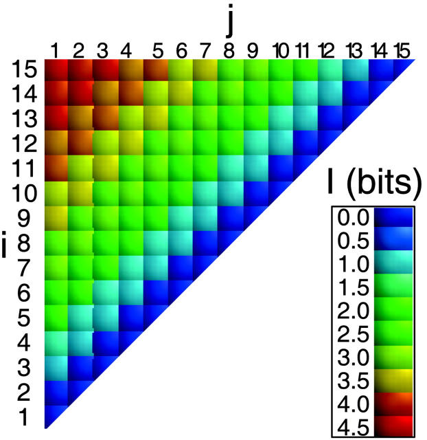
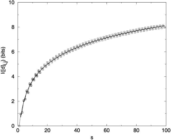
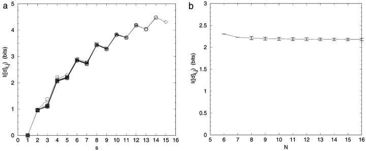
All conformations of a 15-bead chain were enumerated, and the information content of each [d]_i,j, I([d_i,j]), calculated according to Eq. 1, is shown in Fig. 1. As expected, information content increases for [d]_i,j off the diagonal (Chan and Dill, 1990). This trend is seen more clearly in Fig. 2, which replots the information content for the exhaustive ensemble of N = 16 and the stochastic ensemble of N = 100 as a function of s. There is a near-monotonic increase of information with sequence separation that is essentially independent of the chain length (Figs. 2 and 3). For large N, the increase in information with s is well approximated by a logarithmic function (Eq. 14) similar to the Jacobson-Stockmayer equation (Jacobson and Stockmayer, 1950) that computes the loss of entropy for loop closures as a function of loop size.

(14)

FIGURE 1.

Information content, I, for each distance element [d]_i,j for N = 15. Color coded as indicated.

FIGURE 2.

Mean information content as a function of s for single distance elements for ensembles from chains of N = 16 (○)(exhaustive enumeration) and N = 100 (□) (stochastic enumeration of 10,000 conformations). The line fit is given by Eq. 14.

FIGURE 3.

Information content by sequence separation. (a) Mean I[d]_i,j as a function of s_i,j. for single distance elements [d]_i,j, plotted for exhaustive ensembles of N = 4 to N = 16. (b) Independence of information content on chain length or chain position for fixed s_i,j = 5.

Exhaustive enumerations of self-avoiding walks for N = 3 to N = 16, shows the tendency for even sequence separations to be slightly more informative than odd sequence separations (Fig. 3 a). This observation is consistent with even-odd oscillations in other structural features on square lattices (Chan and Dill, 1989) and has no obvious implication for protein structures.

Correlation of constraints

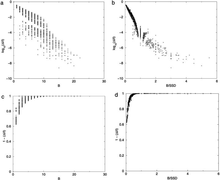
Although the single-most informative distance element is the “end-to-end” sequence separation (1, N for odd N; 1, N − 1 for even N) (Fig. 3 a), finding the most informative set of distance elements is a more complex problem. The principal issue is the overlapping information contained in the distance elements. We begin by examining pairs of distance elements. A related problem has been considered in depth by Chan and Dill (1990), who calculated the entropic losses associated with pairs of prespecified contacts for two- and three-dimensional lattices. In contrast, we examine the nonadditivity (loss) of information for all pairs of distance elements. We develop a numerical relationship that summarizes the average relative loss as a function of the separation of the distance elements. We quantify the correlation by the relative pairwise information reduction for two distance elements [d]_i,j and [d]_i′,j′ defined as:

(15)

This measure is bounded by zero (no loss), if there is no correlation, and unity for complete correlation. In Fig. 4, a–c, the relative loss of information is plotted as a function of (i′,j′) for particular reference values of (i,j) for N = 16. As expected, the loss is greater between elements close to each other in the distance matrix (Chan and Dill, 1990). Fig. 4, d–f, replots the information reduction logarithmically for the same reference distance elements. As the contour lines appear to lie more on the matrix diagonals than on circles about the reference point, we replot the log of the information loss as a function of the city-block sequence distance, B, for all pairs of sequence distance elements for N = 14 (Fig. 5 a). This simple equation explains much of the information loss behavior, with the correlation constant r² = −0.882 for the best-fit line. However, the individual sequence separations, s = s_i,j and s′ = s_i′,j′, also influence the information reduction, where proximal distances with larger s (and thus inherently more information) are reduced relatively more than distances with smaller s. Dividing B by the sum of the sequence separation (SSD), where SSD = s + s′, tightens the correlation (Fig. 5 b), bringing r² = −0.920. Most of the scatter is in the low information-loss (weak correlation) region of the plot. When considering only the points with ΔI/I > 0.001, r² = −0.972. Although the scatter in information loss as a function of these simple distance element transformations appears significant on a logarithmic scale, it is much less significant on a linear scale. In Fig. 5, c and d, (1 − ΔI/I) vs. B shows that at worse, 90% of the joint information is available at a city-block separation of 4 and 95% of the information is available (worst case) at a B of 6.

FIGURE 4.

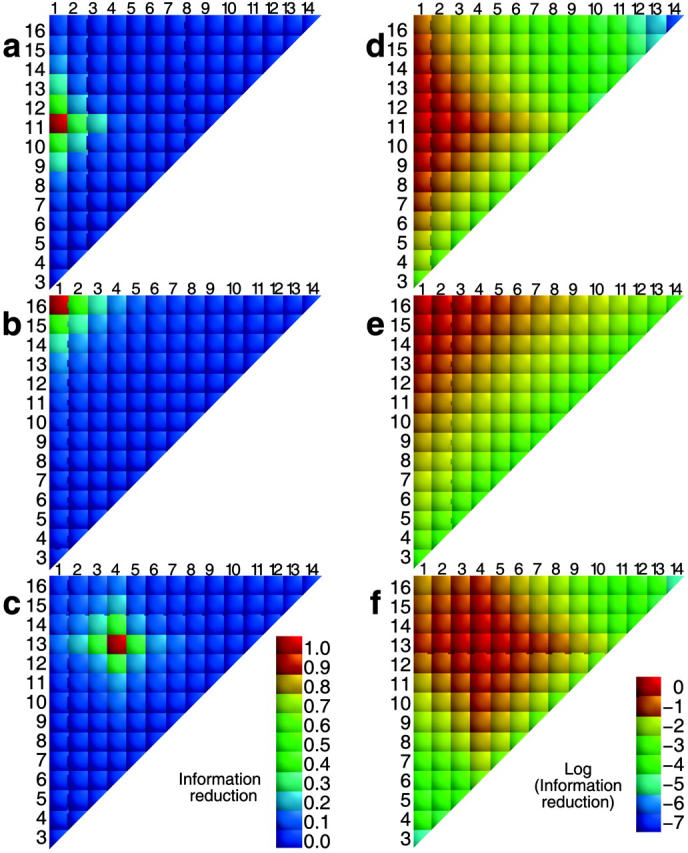
Relative information loss ΔI/I is plotted for all distance elements [d]_i,j., assuming prior knowledge [d]_i,j. Reference [d]_i,j: (1,11) for a and d; (1,16) for b and e; (4,13) for c and f. For a–c, the absolute information loss is plotted, equal to {[I(i,j) + I(i′,j′)] − [I(i,j;i′,j′)]}/[I(i,j;i′,j′)]. In d–f, the decimal logarithm of the information loss is plotted.

FIGURE 5.

Relative information loss, ΔI/I, for all pairs of distances, shown on a log₁₀ scale, calculated by Eq. 14 as a function of transformations of the distance element distances. (a) The x axis is the block element identity distance, B, equal to |i − i′| + |j − j′|. (b) The x axis is B/SSD, where SSD = (s_i,j + s_i′,j′). (c) Plots (1 − [ΔI/I]) versus B. (d) Plots (1 − ΔI/I) vs. B/SSD.

In summary, although we have no simple analytical statement of the information correlation of pairs of Cartesian distances, information loss is dominated by the sequence proximity (loop size) of the beads involved in the two distances, with the loss dropping rapidly for loops whose ends are separated by more than four beads.

Finding the optimal constraint set

The optimal constraint set is defined as the smallest number of exact constraints that partition all the conformers uniquely. Distance-distance correlation makes the problem a difficult one. However, efficient procedures have been developed to construct any specific conformation on 2D and 3D lattices from distance data. Faulon et al. (2002) show that O(n) distances are sufficient for n sites. In this paper we wish to compare arbitrary constraint sets using the Shannon information to quantify the constraint set quality. Specifically, we examine three constraint sets:

1. The globally optimal constraint set: For a prespecified set size, |M|, the globally optimal set of distance constraints, M_global, is determined by measuring I(M) for all possible constraint combinations. Because of computational limitations, this calculation is only possible for small N and small constraint set size |M|.

2. The greedy algorithm constraint set: A less resource-intensive method is a “greedy” algorithm. The constraint set, M_greedy, is calculated by first finding the single most informative distance constraint, [d]_max and then iteratively finding additional maximal constraints. In the case of our lattice models [d]_max is [d]_1,N or [d]_1,N−1 for odd and even length chains, respectively. Of course, this approach has the usual limitations of greedy algorithms (Cormen et al., 2001).

3. The random constraint set: Finally, as a simple control, we measure the information contained in sets of randomly selected distance constraints (Shakhnovich and Gutin, 1990).

Method 1: We calculate I(M) for all possible element combinations

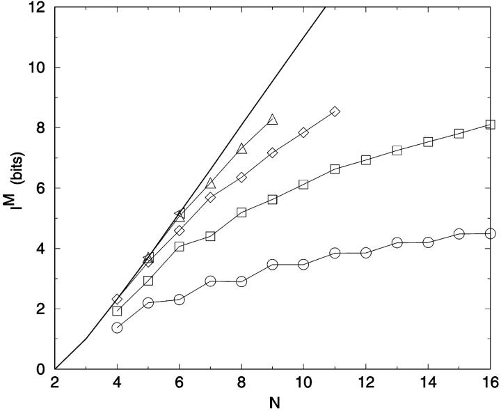
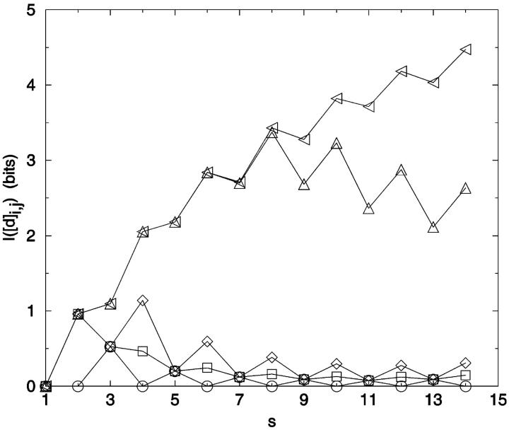
where t is the number of all possible pairings for a bead of length N, equal to ((N − 2) × (N − 1)/2). As noted repeatedly, I(M) is not additive as |M| increases (Fig. 6). One element sets (|M_global| = 1) are the most informative, per constraint, for all chain lengths. For large N and small |M|, the information content of distance constraints approaches simple additivity; e.g., I(M | |M_global| = 2) is 81% greater than I(M | |M_global| = 1), for N = 16. Progressively more constraints yield less information per constraint. Combinatorial exploration of optimum constraints up to |M_global| = 5 is shown in Fig. 6. For reference, I^S for each chain length is also given.

FIGURE 6.

Maximum information I^M for best sets of distance constraints for |M_global| = 1–5 as a function of N. The line represents the maximum information per chain length based on the number of self-avoiding lattice walks (Table 1). ○: 1 distance; □: 2 distances; ⋄: 3 distances; ▵: 4 distances; ◃: 5 distances; —: I^s.

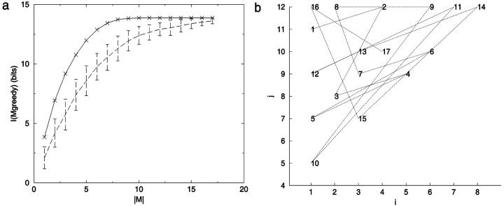
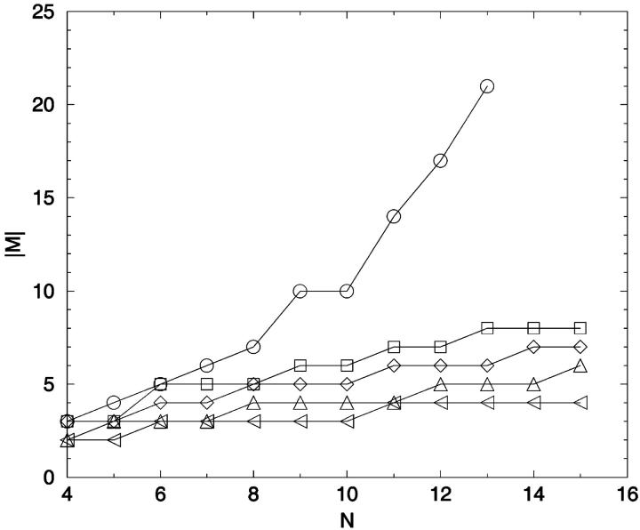
Method 2: The best set of constraints found with the greedy algorithm for the 12-mer chain shows a similar trend (Fig. 7). Fig. 7 a illustrates a problem: the relatively small amount of information contained in the later choices makes the results very path dependent. Fig. 7 b shows the complex evolution of choices as the greedy algorithm explores the distance matrix. Interestingly, much of the information content can be realized with fewer constraints than the N − 2 true degrees of freedom. For example, in a 15-mer chain, 95% of I^S can be encoded through a set of eight distance elements (|M_greedy| = 8) (Fig. 8). The difference between the number of constraints needed to achieve the maximum information and the number needed for a fixed percentage of the information increases exponentially with chain length. To recover I^S completely with the greedy algorithm requires significantly more than N − 2 distance constraints. This discrepancy derives in large part from the imperfect search by such algorithms over all constraint combinations.

FIGURE 7.

Information content dependence on number of constraints. I(M_greedy) was calculated using a greedy algorithm for N = 12. Seventeen distance constraints are required to obtain I^M by this method. (a) I(M_greedy) versus number of distances, |M|. The continuous line serves only to guide the eye. Dashed line I(M_random), averaged over 100 random constraint sets per |M|, with standard deviation given by upper/lower bars. (b) The greedy algorithm choices for |M| = 17 and N = 12 plotted by i,j identity.

FIGURE 8.

Distance constraints for percentage information. The minimum number of distance constraints necessary to retain a given percentage, P, of the ensemble I^S, conformational information, is plotted as a function of chain length. A greedy algorithm was used to calculate the minimum number of distance constraints. P = ○: 100%; □: 95%; ⋄: 90%; ▵: 80%; ◃: 70%.

Method 3: Random selection of constraints performs much worse than the previous two strategies (Fig. 7 a). Nearly twice as many randomly selected constraints are required to achieve the same level of information as those selected by the greedy algorithm.

There are practical issues raised by this analysis. Our calculations are limiting values for the information per constraint. Real systems will be less efficient for many reasons. First, only experiments that can report a range of distance values (e.g., fluorescence labeling, diffraction) can return the maximum amount of information per measurement. Second, only systems in which a significant fraction of all conformers are being sampled can approach the limits shown. More typically, in an experiment on compact states (e.g., native structures of proteins) with a method that is only sensitive to distances within a narrow range (e.g., NMR nuclear Overhauser effect (NOE)) one would expect considerably less information per measurement. Finally, we have been assuming that data are available to sufficient precision to discriminate all distance values for any distance element; “noise” in distance values will reduce the information even further. We explore these points more quantitatively in a later section.

Information content of unlabeled distance constraints

One interesting difference between typical diffraction and NMR experiments on proteins is the “unlabeled” nature of the diffraction data until the “chain tracing” and “phasing” steps occur, whereas, in the NMR studies, assignment of the peaks can be carried out in a largely orthogonal manner to the calculation of tertiary structure. A simple assessment of the information contained in the assignments is available from lattice models of compact states as representatives of folded proteins. We ask what fraction of the total number of conformers have the maximal number of contacts for a given chain length. The ensemble of maximally compact structures contains the contacts that could give rise to (unassigned) NOEs. Each structure contains the same number of contacts. Additional information, beyond just the contact number, is needed to select an individual structure from this set and can be taken as the information to be gained via the assignment procedure for well-folded structures. Values of the maximal number of contacts are simply calculated for square and rectangular Hamilton walks (see Chan and Dill (1989) and below). For example, the number of square Hamilton walks is approximated by W_SHW = 1.40^N−3.90 (Tables 2 and 3), so the additional information to find a unique structure from this set can be estimated as log₂(1.40) or .48 bits/bead (Cejtin et al., 2002; Pande et al., 1994). Attempts have been made to do “real space” assignments from NMR data (Grishaev and Llinas, 2002; Oshiro and Kuntz, 1993). This analysis indicates that any procedural or time-saving advantages of such approaches will carry a cost associated with the loss of orthogonal assignment information.

Information loss from uncertainties in distance constraints

There are three major sources of uncertainty that affect distance measurements: 1), upper/lower bounds on the distance measurements, 2), imprecise distance measurements, and 3), misassignment of distances through incorrect labeling/assignment. Berger et al. (1996, 1999) have studied this last category of error, which we will not discuss here.

Uncertainty gives rise to information loss by preventing discrimination among different conformations. This information loss can often be attributed to the transmission stage of information transfer (Cole, 1993) and is defined as:

(16)

Bound limitations

Consider an upper bound on distances, D_u, such that,

and D_u depends on the physical principles of the experiment and the experimental conditions. For example, because the magnitude of an NOE is proportional to d⁻⁶, NOEs are typically only determined for hydrogen atoms separated by <5 Å. For our lattices, assuming a one-bead to one-residue mapping, detecting an NOE would be equivalent to knowing that two beads are in contact, i.e., separated by the lattice unity distance. Fluorescence energy transfer and chemical cross-link data have longer distance limits. Crystallographic structures have upper bounds set by the smallest diffraction angle that can be observed and lower bounds related to the limit of resolution. We want to calculate the dependence of the information content on the distance detection limit, D_u.

If the particular experiment provides a monotonic relationship between “signal intensity” and “distance,” we can proceed in a straightforward manner to assign distances greater than D_u a lower bound of D_u. For example, it is common practice in some experiments and calculations to report atom pairs as either “contact” (d_i,j ≤ D_u) or “no-contact” (d_i,j > D_u). However, in NMR and FRET the measured signal is a product of both a distance term and an angular correlation term, which can drive the signal close to zero regardless of the distance. To be logically consistent with the underlying physics we must allow for this possibility and give all distances the same lower bound, D_l, for such experiments.

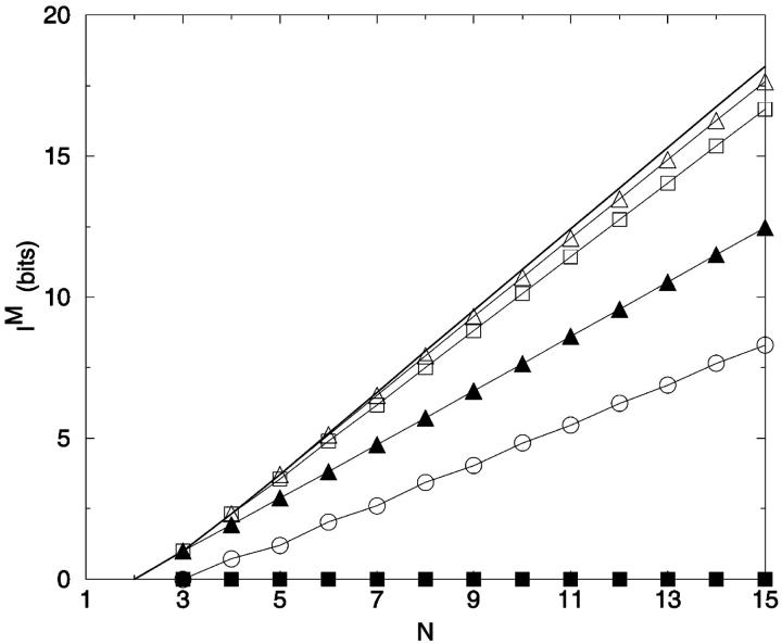
In the first case, where the distance magnitudes are unambiguous, I^M increases linearly for all values of D_u (Fig. 9). I^M for the most limiting contact/no-contact detection limit (D_u = 1) retains nearly half the value of I^S. However, in the second case, where we are not allowed to use “negative” data, the information content of the experiment is much less. I^M equals zero for simple contact/no-contact decisions. Only for D_u ≥ 2, i.e., “next-nearest neighbors,” does such an experiment yield information on the 2D lattice ensemble.

FIGURE 9.

I^M with upper bounds on distances. For the unfilled symbols (○, □, ▵: u = 1, 1.42, 2 units, respectively), I^M is calculated from all interbead distances encoded as d_i,j for d_i,j ≤ u and as equal to u for d_i,j > u. For the filled symbols (▪, ▴: u = 1.42, 2 units respectively), as above, except distances longer than u are treated as unknown. Solid line: No limit.

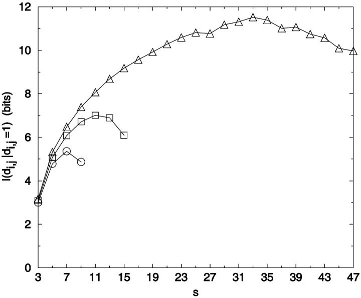
The dependence of I([d]_i,j) on D_u varies with sequence separation (Fig. 10). Information content decreases the most for large sequence separations and low values of D_u. In general, the most informative distance elements have sequence separations of D_u + 2. For example, the most informative contact/no-contact (D_u = 1) distance element occurs at a sequence separation of three, and only yields 0.53 bits. Thus, the information content of knowing that a contact exists, which generally increases with sequence separation (as contacts become more rare with increasing sequence separation) is offset by the loss of the information potential of knowing the distances associated with longer sequence separations. The rarity of contacts at larger sequence separations means that knowing two highly separated residues are in contact is very informative. This is seen in Fig. 11, which plots the information content of knowing two beads (i,j) are in contact (d_i,j = 1) as a function of s_i,j.

FIGURE 10.

Information content, I[d_i,j] by sequence separation with bounded distance detection. Mean information content as a function of sequence separation for single distance constraints is plotted for N = 15 with given distance detection limits, u. Distances are encoded as d_i,j for d_i,j ≤ u and as equal to u for d_i,j > u. ○: 1 unit; □: 1.42 units; ⋄: 2 units; ▵: 6 units; ◃: No limit.

FIGURE 11.

Information content of contact/no contact determinations. The information content of knowing a contact exists (d = 1) is plotted averaged over distance identities of the given sequence separations. Values for even-value sequence distances are not given because these contacts are geometrically unfeasible. ○: 10-mer; □: 16-mer; ▵: 49-mer.

Uncertainty due to limitations in precision of measurements

An issue common to all experiments is the magnitude of the “noise” or imprecision in the measurements. To explore the impact of random noise on the ability to distinguish conformations from one another, we consider two limiting cases for fully enumerated conformational ensembles from 2D lattices. First, we identify conformations most resistant to noise, defined as pairs of conformations that are maximally different and second, in the same ensemble, we find which conformational pairs are most similar. The conventional measures for conformational difference (see Methods section) are the RMS atom-position difference after superposition and the RMS of the distance-difference matrix elements (Levitt, 1976). We will also use the largest element in distance-difference matrix, e^a,b(see Methods).

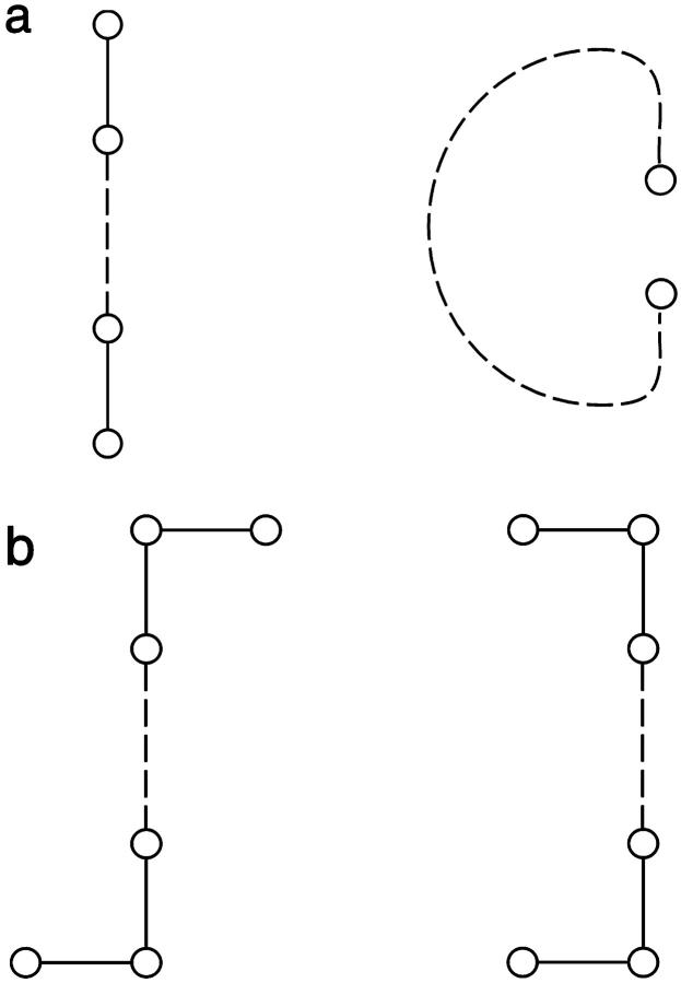
The use of e^a,b yields unexpectedly simple comparisons among chains of different lengths, especially when e^a,b is normalized through division by the chain length, N. The value e^a,b can assume has natural limits. The largest possible distance differences, over all conformational pairs, is in element [d]_1,N (Fig. 12 a). The smallest possible nonzero difference elements likewise occur near [d]_1,N for cases where the bead displacement between two conformations is nearly orthogonal to the interbead vector. For N ≥ 7, the smallest e^a,b over all pairs of d^a and d^b for the ensemble of 2D conformers is in the single conformational pair in Fig. 12 b for which

(17)

FIGURE 12.

Limiting conformations on 2D square lattices. Top pair (a) has the largest e^a,b value (even − N) and the bottom pair (b) illustrates the lowest e^a,b pair (N ≥ 7).

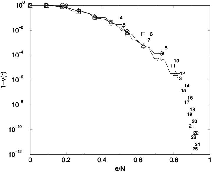
To provide an overview of the distribution of conformer-conformer differences we plot, in Fig. 13, the fraction of distinguishable conformational pairs compared to all conformational pairs, (1 − v(r)), as a function of e^a,b/N for the fully enumerated square lattice walks of size up to N = 13. In addition to these complete distributions, we also show the limiting values for the most similar and most different pairs of conformers for 3 ≤ N ≤ 25. A related plot shows the fraction of indistinguishable conformational pairs compared to all pairs (Fig. 14). Both plots show a remarkable independence from chain length.

FIGURE 13.

Conformational distinguishability. The fraction of distinguishable conformational pairs compared to the total number of conformational pairs, equal to 1-v(r), (see text) is plotted as a function of the relative noise, equal to r = e/N. ○: 3-mer; ▵: 6-mer; ▹: 9-mer; ^*: 12-mer; ○: 13-mer.

FIGURE 14.

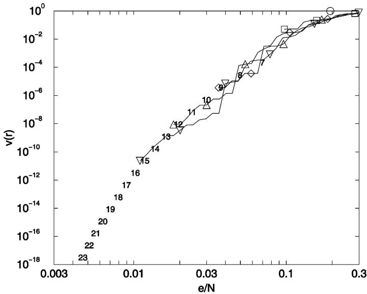
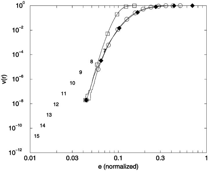
Conformational indistinguishability. v(r) is plotted as a function of the relative uncertainty, r = e/N. The limiting threshold noise levels for ensembles N = 7–23 are given by ensemble identity, N, and are placed at x = {[(N − 3)² + 4]^1/2 − (N − 3)}/N, y = 2/[W × (W − 1)] which are the limiting relative noise levels and inverse of total number of conformational pairs, respectively. ○: 3-mer; □: 6-mer; ⋄: 9-mer; ▵: 12-mer; ▿: 15-mer; 7–23: Limiting errors for 7–23 mers.

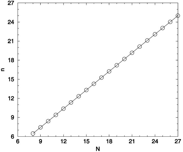
There are several features of Fig. 14 that are useful for our analysis. First, as noted earlier, v(r) can be thought of as a cumulative distance distribution function for pairs of conformations on specific lattices. It provides, when normalized, the fraction of the ensemble within a specific error, or conformational distance, of a given conformation, averaged over all ensemble members. It also provides a visualization of the impact of noise on the ability to discriminate one conformer from all the others. Additionally, we can calculate the marginal dimensionality, n, from Fig. 14 by computing the slope of the line passing through the points for limiting conformational pairs from the ensembles of length N − 1 and N + 1. We find, for 2D square lattices, that the limiting marginal dimensionality is nearly equal to N − 2, the true number of mechanical degrees of freedom for these walks (Fig. 15). This value for the slope can also be derived directly from the formulas given in the legend of Fig. 14, assuming N ≫ 1. Following this idea one step further, we can interpret the slope at all points on Fig. 14 as the number of degrees of freedom that are effective in producing the conformational differences associated with a particular (normalized) displacement.

FIGURE 15.

The marginal dimensionality, n, is plotted as a function of the chain length, N. The marginal dimensionality for N was calculated from the logarithmic slope between the two points for N − 1 and N + 1 in Fig. 14.

Effect of uncertainty on compact lattice structures

The properties of the fully enumerated ensembles are dominated by extended conformers analogous to denatured states of proteins. To provide insight into arguably more biologically relevant ensembles such as the native and molten globule protein states (Chan and Dill, 1989), we studied the subset of compact conformers by generating perfect-square Hamilton walks where every lattice site is occupied. We exhaustively enumerated square Hamilton walks up to N = 49 (Table 2).

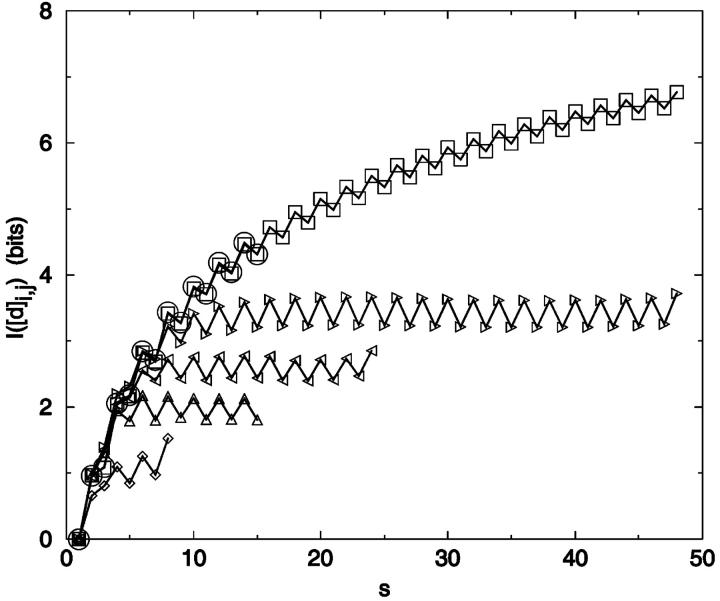
The dependence of information content on bead sequence separation is fundamentally different in square Hamilton walk ensembles compared to full enumeration ensembles (Fig. 16; compare to Figs. 2 and 3). In the latter case, as we saw, I([d]_i,j) depends exclusively on sequence separation. For Hamilton walks, I([d]_i,j) also depends on N, but it becomes nearly constant for sequence separations greater than ∼N^1/2. This result agrees with the expectation that positional correlation between beads i and j is constant for sequence separations greater than the diagonal distance, which increases as ∼N^1/2.

FIGURE 16.

Mean information content for Hamilton square walks as a function of sequence separation for single distance constraints (N = 9, 16, 25, 49), a full enumeration ensemble (FE) (N = 16) and a stochastic, nonexhaustive ensemble of unconstrained conformations (FES) (N = 49). ○: 16-mer FE unit; □: 49-mer FES; ⋄: 9-mer HW; ▵: 16-mer HW; ◃: 25-mer HW; ▹: 49-mer HW.

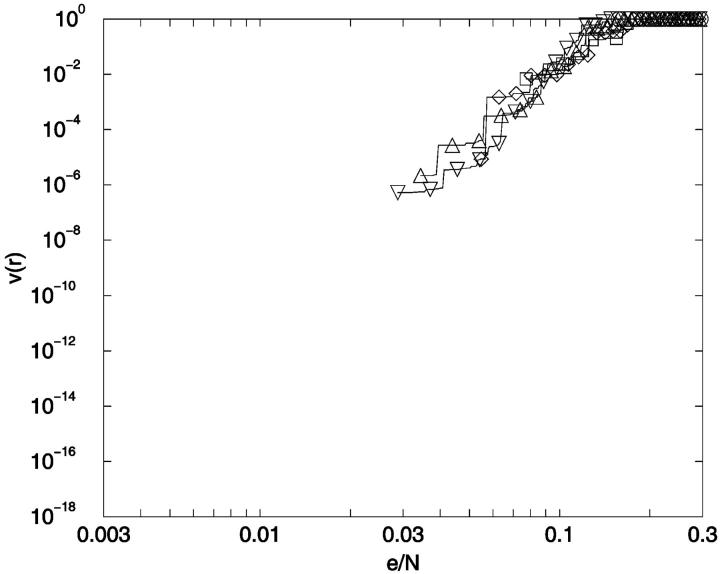
We also calculated v(r) as a function of e^ab/N for the Hamilton walk ensembles (Fig. 17). The curves are surprisingly similar to the fully enumerated walks (Fig. 14), even though the Hamilton walk ensembles sample only a small subset of full enumeration conformational space and have additional degeneracy. For example, in the N = 36 Hamilton walk ensemble, 3608 pairs of conformations become indistinguishable with an absolute uncertainty of 1.24 (equal to ) or relative uncertainty of 0.0343.

FIGURE 17.

Conformational indistinguishability for Hamilton walks. v(r) is plotted as a function of the relative noise, e/N, for the Hamilton walk constrained ensembles (see Fig. 14). ○: 9-mer; □: 16-mer; ⋄: 25-mer; ▵: 36-mer; ▿: 49-mer.

The full enumeration ensembles, discussed previously, have limiting characteristics largely governed by simple relationships among extended conformations. None of these situations arises when the ensemble of interest is restricted to compact conformers. Thus it is not clear at this point whether the similarity in (normalized) pair distributions arises from some fundamental principle or from specific geometric constraints.

We note that the pair distributions show multimodal character (notice the small break in the curve near e^ab/N = 0.03 in Fig. 14), as we saw in our earlier work on nonlattice chains (Sullivan and Kuntz, 2001). Very similar v(r) distributions are obtained using off-lattice polyalanine chains (Fig. 18). Note that the 30 residue chains with 58 dihedral degrees of freedom closely approximate the distribution from a stochastic sampling of a 60 bead (58 degrees of freedom) 2D lattice walk.

FIGURE 18.

Conformational indistinguishability for stochastic polyalanine ensembles (see text and Fig. 14). ○: Yarn 30 extended; □: Yarn 30 compact; ♦: 2D lattice stochastic N = 60; Numbered points 7–15: Limiting distances for N = 7–15 for 2D extended walks (see Fig. 14). Yarn e values are divided by 3.8N. 2D lattice e values are divided by N.

Relating information loss to noise

Extracting a relationship between information loss and noise requires a detailed model of how noisy messages are misread. One such model uses the “noise sphere” concept outlined in the Methods section. Briefly, a set of W distinct messages, {w_i}, becomes scrambled as noise is introduced and some messages become indistinguishable. Note that this approach requires that after the noise has been introduced, every conformer still be a proper member of the set; distorted (off-lattice) geometries are not allowed. We define a “noise sphere” in which conformations w_j that are within a hypersphere of radius r centered about conformation w_i are indistinguishable. The radius r can be associated with any measure of noise and formulated with any explicit error distribution function: we use either RMSD or e^a,b and assume a uniform distribution of noise.

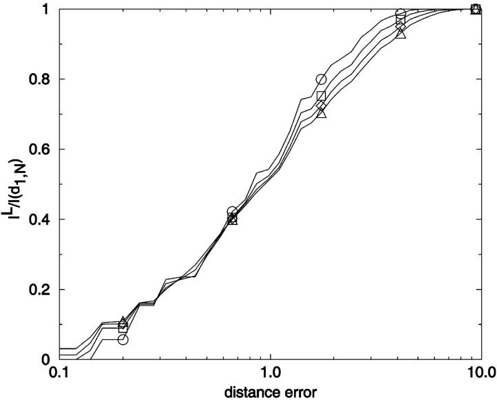
This procedure can be used for entire conformations, but as noted in the methods section, it is also directly applicable to information loss for individual constraints or sets of constraints. In Fig. 19 we show the fractional information loss for the [d]_1,N distance element for 2D chains as a logarithmic function of the noise magnitude that we take as the noise sphere radius. Although there is some small dependence of normalized loss on the chain length, the curves indicate a smooth relationship with half of the information lost when the noise magnitude is equal to the lattice spacing.

FIGURE 19.

Relative information loss for [d]_1,N, full enumeration ensemble, for N = 9 (○), 11 (□), 13 (⋄), 15 (▵), 15 (▵).

For 2D lattice walk ensembles, the relationship between information loss per degree of freedom and e^a,b (derived via Eq. 10) is shown in Fig. 20 a. The curves relating information loss and coordinate RMSD for the same ensembles are shown in Fig. 20 b. Fig. 21 shows similar plots for Hamilton walks. At very low noise magnitudes, there is no information loss, as expected for a set of discrete conformers. As the noise increases beyond a critical value, there is a region of barely perceptible loss as the most similar conformers are merged. At some point, increasing error causes major information loss because many conformations populate the average noise sphere. Finally at large noise levels, there is a slow loss of information because only the most different conformers are left to merge.

FIGURE 20.

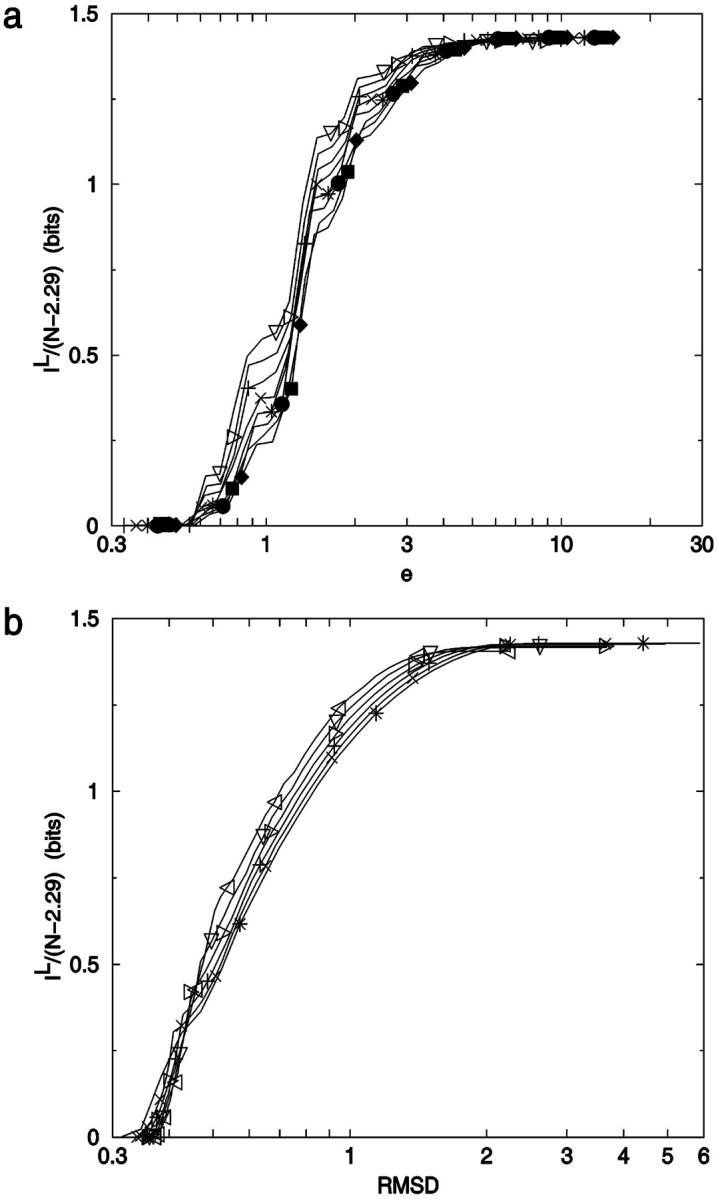
Information loss per degree of freedom for full enumeration, for N = 7 (◃), 8 (▿), 9 (▹), 10 (+), 11 (×), 12 (^*), 13 (•), 14 (▪), 15 (♦). The factor (N − 2.29) comes from I^S = 1.43(N − 2.29), a recasting of the self-avoiding walk equation for W(N) in Table 3. (a) Plotted against e. (b) Plotted against coordinate RMSD.

FIGURE 21.

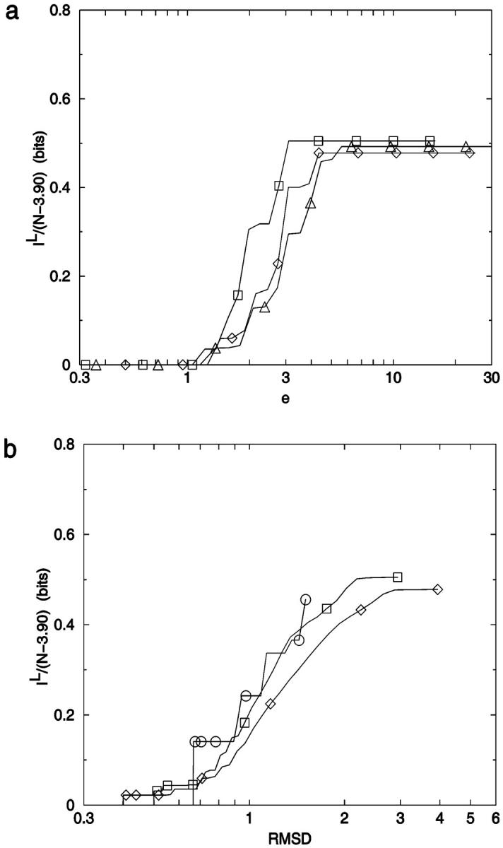
Information loss per degree of freedom for compact two-dimensional lattice structures for N = 16 (□), 25 (⋄), 36 (▵). (a) Plotted against e. (b) Plotted against coordinate RMSD.

To summarize this section: the noise sphere model allows a straightforward treatment of the effect of noise on information content for individual distance elements, sets of distance constraints, and full enumeration conformational ensembles. Not surprisingly, the information loss/noise curves are the steepest when the noise magnitude is near the lattice spacing. Most of the chain length dependence can be removed by reporting information per residue, which is sensibly constant at longer chain lengths.

Information per constraint

As a practical matter, experimentalists are interested in how much information can be extracted from a necessarily limited set of measurements. This question has been addressed at various levels of sophistication by many authors. For example, Shakhnovich and Gutin, (1990) have studied a model of polymer chains where the entropy loss on random cross-linking yields a leading term proportional to the number of cross-links per residue. Our analysis of exact constraints on fully enumerated conformers also yields some limiting answers. For a 2D self-avoiding walk on a square lattice a single optimal measurement can provide ∼log₂N bits (Figs. 2 and 3) whereas N beads can be fixed on the lattice with N − 2 constraints for any given conformer, or ∼1.5 bits/constraint. Compact structures, such as the 2D Hamilton walks, can yield even more information per constraint (Fig. 11). If the optimal set of constraints is not available, more measurements are needed. For example, for N = 12, 17 constraints are needed to supply 14 bits or 0.8 bits/constraint (Fig. 7). If constraints are chosen randomly, many more would be required to supply the same information. Thus, for exact (noise-free) constraints, one might expect ∼0.5 bits/constraint over a random set of measurements. Shakhnovich and Gutin give similar numerical results when converted into the same units. They report 0.5–1.5 bits/constraint over the chain lengths we consider.

If we turn to constraints that contain random noise, the information content decreases further. Using Fig. 19 we can estimate that noise levels of ∼0.1 lattice units for individual distance constraints cost less than 10% of the information per residue, whereas noise levels comparable to the lattice spacing would require doubling the number of constraints to achieve the same information content as noise-free measurements. For noise levels greater than the lattice spacing, the information content per residue diminishes very rapidly. Fig. 19 suggests that at noise levels of twice the lattice length, five times as many constraints would be needed compared to the exact constraints. These numbers are, of course, very approximate guides. Presumably, an analogous estimate would apply to nonlattice models of polymers as long as discrete conformers can be enumerated. For polypeptide chains, the results of Troyer and Cohen (1995) imply an absolute minimum separation of ∼0.1 Å per residue or a relative separation of 0.001 Å per residue² for a 100 residue protein. These limiting “conformational radii” are quite comparable to those for the most similar conformers in 2D lattice walks of the same length derived from Eq. 17.

In summary, by considering the effects of noise on single distances, we are able to make estimates of how much additional effort is required, in a best-case scenario, to overcome the information loss due to random noise in measurements.

DISCUSSION

Developing a general and quantitative treatment of information content for macromolecular ensembles raises both fundamental and practical issues. One serious concern is the need for enumeration of the conformations. Exhaustive enumeration will always be limited by computational resources and is not applicable to off-lattice models for the foreseeable future (Sullivan and Kuntz, 2001). Feldman and Hogue's more optimistic view (Feldman and Hogue, 2002) is based on the extreme value distribution function that may overestimate the number of structures at small RMSD. The real goal for off-lattice structures is an analytic distribution function with sufficient accuracy to derive thermodynamic properties. The relative simplicity of the v(r) vs. e curves offers some hope that such functions can be devised, although the multimodal character of the curves indicates that direct stochastic sampling may not suffice to probe the most closely related conformers.

The data for various lattice and off-lattice systems (Table 3) raises the question of what reference state is most appropriate for comparisons among different models. The most obvious choice is an unconstrained ideal gas. This is roughly analogous to measuring thermodynamic energies using E = mc²; it gives the right answers in a very awkward form. The important point is that the choice of lattice and lattice move set (or any other prior constraints) influences the information content of the resulting ensemble, with varying amounts of residual information (entropy) being associated with the set of choices.

The application of noise theory requires the development of parametric noise models and a set of choices for parameter values. There is currently little guidance from physical principles for choosing error metrics and clustering methods. We elected to use a very simple formulation of the problem based on the application of the noise sphere model to fully enumerated lattice ensembles. We postpone a treatment of energetic differences among conformers, although they could be put directly into Eq. 10 as population weights. We assume the noise to be white noise, which implies uniform probability of “scrambling” for all conformers within the noise sphere. More realistic, distance-dependent noise functions could also be readily incorporated. We chose displacement measures pragmatically rather than attempting a full physical analysis. We noted earlier that the noise sphere model is formally adapted to accept other displacement metrics. More sophisticated entropic clustering models are available from information theory (Guiasu, 1977). However, their computational complexity is extremely high, and they are not practicable even for small 2D ensembles.

Although our specific results for the information per constraint and information lost as a function of noise are limited to the ensembles studied, the general features of these curves can provide useful insight into experimental design. It certainly should be possible to extend these ideas to proteins and nucleic acid polymers. In situations where diverse types of data are used and noise propagation is poorly understood, maximum-information optimization using hypothetical models of transmission errors could help determine which combinations of various measurements are most informative. This would be a first attempt toward improving the utility of measurements in such systems, a critical step if we are to improve the quality and speed of current structure determination methods (Rabitz, 1989).

CONCLUSIONS

1. Information content of distance constraints increases as the log of the sequence separation for all systems studied except square Hamilton walks where a limiting value is reached as the sequence separation reaches √N.

2. Although a single noise-free distance constraint, namely the end-to-end distance, can select individual conformers from an ensemble and construction methods exist that use as few as N − 2 distance constraints per conformer, the size of the set of constraints needed to uniquely partition the entire ensemble is not known in a general way. The problem is inherently complex (Chan and Dill, 1990) arising from correlations among distance elements that are largely local in sequence space. We show that a simple greedy algorithm can supply an arbitrarily high percentage of the total information (e.g., 95%) with many fewer than N − 2 constraints. On a practical level, randomly selected exact constraints provide much less information, which we estimate to be 0.5 bits/constraint, on the average, for 2D lattice ensembles.

3. Using the “noise sphere” model, we show that noise reduces information content in a surprisingly universal way for fully enumerated lattice walks and maximally compact Hamilton square walks. It is not possible to use the same model for off-lattice ensembles without some method of estimating the total number of conformations.

4. The slope of the information loss versus noise curves can be directly related to the number of active or “effective” degrees of freedom for the ensemble.

5. A complete quantitative treatment of information content is surprisingly difficult. Many technical issues arise that involve additional assumptions that influence the numerical results. These issues include: choice of potential functions, clustering methods, and noise distribution functions among others. There is currently little guidance from physical principles or experiment for this selection. More work is needed to clarify the best way to extend these studies to off-lattice ensembles.

References

- Berger, B., J. Kleinberg, and T. Leighton. 1996. Reconstructing a three-dimensional model with arbitrary errors. Proceedings of the ACM Symposium on Theory of Computing. Philadelphia, PA. 449–458.
- Berger, B., J. Kleinberg, and T. Leighton. 1999. Reconstructing a three-dimensional model with arbitrary errors. Journal of the ACM. 46:212–235. [Google Scholar]
- Brunger, A. T., G. M. Clore, A. M. Gronenborn, R. Saffrich, and M. Nilges. 1993. Assessing the quality of solution nuclear magnetic resonance structures by complete cross-validation. Science. 261:328–331. [DOI] [PubMed] [Google Scholar]
- Cejtin, H., J. Edler, A. Gottlieb, R. Helling, L. Hao, J. Philbin, W. Ned, and T. Chao. 2002. Fast tree search for enumeration of a lattice model of protein folding. J. Chem. Phys. 116:352–359. [Google Scholar]
- Chan, H. S., and K. A. Dill. 1989. Compact polymers. Macromolecules. 22:4559–4573. [Google Scholar]
- Chan, H. S., and K. A. Dill. 1990. The effect of internal constraints on the configurations of chain molecules. J. Chem. Phys. 92:3118–3135. [Google Scholar]
- Chan, H. S., and K. A. Dill. 1991. Polymer principles in protein structure and stability. Annu. Rev. Biophys. Biophys. Chem. 20:447–490. [DOI] [PubMed] [Google Scholar]
- Chorev, M., and M. Goodman. 1995. Recent developments in retro peptides and proteins - an ongoing topochemical exploration. Trends Biotechnol. 13:438–445. [DOI] [PubMed] [Google Scholar]
- Choy, W. Y., and J. D. Forman-Kay. 2001. Calculation of ensembles of structures representing the unfolded state of an SH3 domain. J. Mol. Biol. 308:1011–1032. [DOI] [PubMed] [Google Scholar]
- Cole, C. 1993. Shannon revisited: information in terms of uncertainty. J. Am. Soc. Inf. Sci. 44:204–211. [Google Scholar]
- Cormen, T. H., C. E. Leiserson, and R. L. Rivest. 2001. Introduction to Algorithms. MIT Press.
- Cooper, A. 1999. Thermodynamics of protein folding and stability. In Protein. G. Allen, editor. JAI Press, Stamford, CT. 217–270.
- Crippen, G. M. 2000. Enumeration of cubic lattice walks by contact class. J. Chem. Phys. 112:11065–11068. [Google Scholar]
- Crippen, G. M., and T. F. Havel. 1988. Distance Geometry and Molecular Conformation. Wiley, New York
- Dill, K. A. 1985. Theory for folding and stability of globular proteins. Biochemistry. 24:1501–1509. [DOI] [PubMed] [Google Scholar]
- Dill, K. A., S. Bromberg, K. Yue, K. M. Fiebig, D. P. Yee, P. D. Thomas, and H. S. Chan. 1995. Principles of protein folding–a perspective from simple exact models. Protein Sci. 4:561–602. [DOI] [PMC free article] [PubMed] [Google Scholar]
- Dobson, C. M., A. Sali, and M. Karplus. 1998. Protein folding: a perspective from theory and experiment. Angew. Chem. Int. Ed. Engl. 37:868–893. [DOI] [PubMed] [Google Scholar]
- Faulon, J. L., M. D. Rintoul, and M. M. Young. 2002. Constrained walks and self-avoiding walks: implications for protein structure determination. Journal of Physics A-Mathematical & General. 35:1–19. [Google Scholar]
- Feldman, H. J., and C. W. Hogue. 2002. Probabilistic sampling of protein conformations: new hope for brute force? Proteins. 46:8–23. [PubMed] [Google Scholar]
- Flory, P. J. 1953. Principles of Polymer Chemistry. Cornell University Press, New York
- Gregoret, L. M., and F. E. Cohen. 1990. Novel method for the rapid evaluation of packing in protein structures. J. Mol. Biol. 211:959–974. [DOI] [PubMed] [Google Scholar]
- Gregoret, L. M., and F. E. Cohen. 1991. Protein folding. Effect of packing density on chain conformation. J. Mol. Biol. 219:109–122. [DOI] [PubMed] [Google Scholar]
- Grishaev, A., and M. Llinas. 2002. Protein structure elucidation from NMR proton densities. Proc. Natl. Acad. Sci. USA. 99:6713–6718. [DOI] [PMC free article] [PubMed] [Google Scholar]
- Guiasu, S. 1977. Information Theory with Applications. McGraw-Hill
- Gutin, A. M., and E. I. Shakhnovich. 1994. Statistical mechanics of polymers with distance constraints. J. Chem. Phys. 100:5290–5293. [Google Scholar]
- Havel, T. F., I. D. Kuntz, and G. M. Crippen. 1983. The theory and practice of distance geometry. Bull. Math. Biol. 45:665–720. [Google Scholar]
- Irback, A., and C. Troein. 2002. Enumerating designing sequences in the HP model. Journal of Biological Physics. 28:1–15. [DOI] [PMC free article] [PubMed] [Google Scholar]
- Levitt, M. 1976. A simplified representation of protein conformations for rapid simulation of protein folding. J. Mol. Biol. 104:59–107. [DOI] [PubMed] [Google Scholar]
- Levy, R. M., M. Karplus, J. Kushick, and D. Perahia. 1984. Evaluation of configurational entropy for proteins: application to molecular dynamics simulations of an α-helix. Macromolecules. 17:1370–1374. [Google Scholar]
- Luo, H. B., and K. Sharp. 2002. On the calculation of absolute macromolecular binding free energies. Proc. Natl. Acad. Sci. USA. 99:10399–10404. [DOI] [PMC free article] [PubMed] [Google Scholar]
- Oshiro, C. M., and I. D. Kuntz. 1993. Application of distance geometry to the proton assignment problem. Biopolymers. 33:107–115. [DOI] [PubMed] [Google Scholar]
- Pande, V. S., C. Joerg, A. Y. Grosberg, and T. Tanaka. 1994. Enumerations of the Hamiltonian walks on a cubic sublattice. Journal of Physics A. 27:6231–6236. [Google Scholar]
- Potter, M. J., and M. K. Gilson. 2002. Coordinate systems and the calculation of molecular properties. Journal of Physical Chemistry A. 106:563–566. [Google Scholar]
- Rabitz, H. 1989. Systems analysis at the molecular scale. Science. 246:221–226. [DOI] [PubMed] [Google Scholar]
- Rosenbluth, M. N., and A. W. Rosenbluth. 1955. Monte Carlo calculation of the average extension of molecular chains. J. Chem. Phys. 23:356–359. [Google Scholar]
- Schafer, H., X. Daura, A. E. Mark, and W. F. van Gunsteren. 2001. Entropy calculations on a reversibly folding peptide: changes in solute free energy cannot explain folding behavior. Proteins. 43:45–56. [DOI] [PubMed] [Google Scholar]
- Schafer, H., A. E. Mark, and W. F. Van Gunsteren. 2000. Absolute entropies from molecular dynamics simulation trajectories. J. Chem. Phys. 113:7809–7817. [Google Scholar]
- Schlitter, J. 1993. Estimation of absolute and relative entropies of macromolecules using the covariance matrix. Chem. Phys. Lett. 215:617–621. [Google Scholar]
- Shakhnovich, E., and A. Gutin. 1990. Enumeration of all compact conformations of copolymers with random sequence of links. J. Chem. Phys. 93:5967–5971. [Google Scholar]
- Shannon, C. E. 1948. A mathematical theory of communication. The Bell System Technical Journal. 27:379–423; 623–656. [Google Scholar]
- Sibbald, P. R. 1995. Deducing protein structures using logic programming: exploiting minimum data of diverse types. J. Theor. Biol. 173:361–375. [DOI] [PubMed] [Google Scholar]
- Sullivan, D. C., and I. D. Kuntz. 2001. Conformation spaces of proteins. Proteins. 42:495–511. [PubMed] [Google Scholar]
- Troyer, J. M., and F. E. Cohen. 1995. Protein conformational landscapes: energy minimization and clustering of a long molecular dynamics trajectory. Proteins. 23:97–110. [DOI] [PubMed] [Google Scholar]
- Wang, Z. H., M. B. Luo, and J. M. Xu. 1999. Conformational entropy of self-avoiding polymer chains. European Polymer Journal. 35:973–975. [Google Scholar]
- Young, J. F. 1971. Information Theory. Butterworth & Company Ltd., Bristol