Water and Proton Conduction through Carbon Nanotubes as Models for Biological Channels

Abstract

Carbon nanotubes, unmodified (pristine) and modified through charged atoms, were simulated in water, and their water conduction rates determined. The conducted water inside the nanotubes was found to exhibit a strong ordering of its dipole moments. In pristine nanotubes the water dipoles adopt a single orientation along the tube axis with a low flipping rate between the two possible alignments. Modification can induce in nanotubes a bipolar ordering as previously observed in biological water channels. Network thermodynamics was applied to investigate proton conduction through the nanotubes.

INTRODUCTION

Since the discovery of carbon nanotubes (Iijima, 1991), extensive studies have been carried out on this novel material, and many of its interesting properties have been revealed. Carbon nanotubes (CNTs) promise various technical applications, e.g., in making nanoscale electronic devices (Wind et al., 2002) or microscopic filters (Miller et al., 2001). CNTs can be manufactured in various sizes, with diameters ranging from less than 1 nm to more than 100 nm. CNTs can attach to each other and form bundles by self-alignment (Dresselhaus et al., 1996). CNTs may be protonated (O'Connell et al., 2002), and some may have charged atomic sites (Miller et al., 2001).

Computational studies have suggested that CNTs can be designed as molecular channels to transport water. A (6,6) single-walled CNT, with a diameter of 8.1 Å, has been studied recently by molecular dynamics (MD) simulations (Hummer et al., 2001). The simulations revealed that the CNT was spontaneously filled with a single file of water molecules and that water diffused through the tube concertedly at a fast rate. The motion of water through CNTs can be described by a continuous-time, single-file random-walk model (Berezhkovskii and Hummer, 2002).

Microporous alumina layers with CNTs embedded within the pores can be produced by chemical vapor deposition and fluxes of electrolytes through these layers have been observed (Miller et al., 2001). Chemical groups can be attached to the CNTs by electrochemical derivatization, which can alter their transport properties (Miller et al., 2001). The findings suggest applications for CNTs as nanofluidic devices, e.g., filters.

In living cells exist analogous water channels. Most notable are aquaporins (AQPs), a family of membrane channel proteins, that are abundantly present in nearly all life forms (Borgnia et al., 1999). Biological water channels are much more complex than CNTs, with irregular surfaces and highly inhomogeneous charge distributions. CNTs can serve as prototypes for these biological channels, that can be investigated more easily by MD simulations due to their simplicity, stability, and small size. But pristine CNTs are electrically neutral, and unable to reproduce some important features of biological channels. For example, MD simulations have revealed that water molecules in the AQP channels adopt a bipolar orientation which is induced electrostatically and is linked to the exclusion of proton conduction in AQP channels (Tajkhorshid et al., 2002). However, one may modify CNTs through the introduction of charges to mimic AQP water channels. Below we describe how we have modeled accordingly several types of CNTs with representative charge distributions by means of MD simulations. We have investigated, in particular, the effect of charges on water conduction and water orientation. We also investigated proton conduction through the CNTs using the theory of network thermodynamics (Brünger et al., 1983; Schulten and Schulten, 1985, 1986).

METHODS

A periodic system containing 12 hexagonally-packed identical CNTs sandwiched by bulk water per unit cell has been simulated. Fig. 1 shows the unit cell of this system. Each CNT (144 atoms) is of (6,6) armchair type, and has a C–C diameter of 8.2 Å and a length of 13.4 Å. A single copy of the same CNT was studied in Hummer et al. (2001). We include multiple CNTs in the unit cell to avoid possible “image” effects between conducted water. The unit cell contains a total of 6348 atoms.

FIGURE 1.

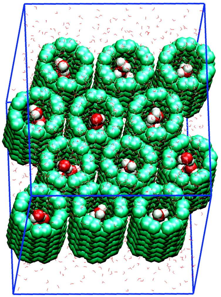
Unit cell of a system of twelve carbon nanotubes and 1540 water molecules. Carbon nanotubes and conducted water molecules (inside the tubes) are rendered through VDW spheres; bulk water is rendered through thin lines.

The parameters for carbon atoms of CNTs were those of type CA in the CHARMM force field (MacKerell Jr. et al., 1998), which was designed for benzene. The TIP3P water model (Jorgensen et al., 1983) was used. Four types of CNTs were simulated in this study, which we will refer to as nt0, ntP0N, ntNPN, and ntPNP below. In nt0 (pristine CNT), all atoms have zero charge. In ntP0N, two atoms at one end of the CNT were each assigned a charge of +0.25 e, resulting in a total charge of +0.5 e at that end; similarly, at the other end, two atoms were given a total charge of −0.5 e. In ntNPN, at each end, two atoms have a total charge of −0.5 e; in addition, two atoms in the middle of the CNT were given a total charge of +1 e. In ntPNP, the charge distribution was opposite to that in ntNPN, with +0.5 e net charges at each end and −1 e in the middle. Table 1 summarizes the charges on these CNTs. We note that the total charge of each type is zero.

TABLE 1.

Charge distributions in the four types of CNTs studied in this article

	End	Middle	End
nt0	0	0	0
ntP0N	+0.5	0	−0.5
ntNPN	−0.5	+1	−0.5
ntPNP	+0.5	−1	+0.5

The magnitude of the assigned charges mentioned above is chosen to generate an electrostatic field comparable to that in biological channels. It is known that an α-helix has a net dipole moment whose magnitude corresponds to a charge of ∼0.5–0.7 e at each end of the helix (Branden and Tooze, 1991). In ntNPN and ntPNP, the dipole moments of two halves of the CNT are similar to those of two oppositely oriented α-helices with one-half of the CNT length; in ntP0N, the net dipole moment mimics that of a single α-helix with the same length as the CNT. In these modified CNTs, we assign the charges to only a few carbon atoms rather than distributing them over many, in an attempt to mimic charged groups in biological channels such as AQPs, which usually have strong localized interaction with water molecules inside the channels. In the following, the simulations on nt0, ntP0N, ntNPN, and ntPNP are referred to as sim0, simP0N, simNPN, and simPNP, respectively.

All simulations were performed at constant temperature (300 K) and pressure (1 atm), and by using the PME method (Essmann et al., 1995) for full electrostatics. Each of the four systems described above was simulated for 10 ns, with coordinates recorded every 1 ps. The first 200-ps of each simulation was discarded, and the rest of the trajectory was used for analysis. Version 2.5 of the program NAMD2 (Kalé et al., 1999) was used for the simulations, with a performance of ∼12.6 h per ns on 16 processors of an IA-64 Linux cluster.

During the simulations, translation of the CNTs due to thermal fluctuation was observed. However, their aggregation remained very stable and the CNTs translated only collectively. All of the CNTs were empty initially, but filled up with water molecules within 200 ps. Water did not enter the gaps between CNTs, because in the chosen arrangement, the gaps were too narrow to accommodate water molecules (distance of 2.5 Å from gap center to nearest carbon atom).

RESULTS

In this section, we will first describe and quantify water diffusion and orientation observed in the simulations of each type of CNTs. Then we will use network thermodynamics (Brünger et al., 1983; Schulten and Schulten, 1985, 1986) to study proton conduction in nt0 and to demonstrate how a bipolar arrangement of water in ntNPN prevents proton conduction.

Water diffusion and orientation

Water molecules entering the CNTs form single files and move concertedly. Such water movement has been characterized by a continuous-time random-walk model (Berezhkovskii and Hummer, 2002). The key parameter in this model, the hopping rate k (a hop is the translocation of the water file by a distance of the separation of adjacent water molecules), has been determined in our simulations and is provided in Table 2. According to the continuous-time random-walk model, the number p of permeation events (a water molecule crossing from one end to the other end of a CNT) per CNT, per ns, can be calculated from k (see Eq. A1 in the Appendix). Alternatively, p can be counted from the trajectories. Both the predicted and directly observed p-values from the simulations are listed in Table 2, where one can see that they are in agreement. The same pristine CNT (nt0) was studied in (Berezhkovskii and Hummer, 2002; Hummer et al., 2001; Kalra et al., 2003) by MD using the AMBER force field, which gave mean hopping times (τ = 1/k) of 13 ps for a single CNT in water (Berezhkovskii and Hummer, 2002; Hummer et al., 2001) and 20 ps for a layer of CNT arrays (Kalra et al., 2003). In sim0 we observed a larger τ-value (37 ps), which may be due to the difference in the force fields (AMBER vs. CHARMM) used. Indeed, it was pointed out in Hummer et al. (2001) that the observed water behavior in CNTs is sensitive to the force field parameters. In comparison with biological channels, the conduction rate in sim0 (5.9 water permeation events per CNT per ns) is more than five times larger than that observed in simulations of AQPs (de Groot and Grubmüller, 2001; Tajkhorshid et al., 2002). This difference is due to the difference in the electrostatic environment in CNTs and AQPs. Indeed, among the four types of CNTs, the pristine CNT (nt0) has the fastest water conduction; in ntNPN, which resembles AQPs more closely, the water molecules exhibited remarkably lower mobility, with no permeation event and only a few hops of water observed in 10 ns.

TABLE 2.

Summary of water permeation in sim0, simP0N, and simPNP

							Observed p (no./ns)
	D (Å2/ps)	K (/ps)	k0 (/ps)	τ (ps)	Predicted p (no./ns)	Total counts	Mean	SD
sim0	0.091	0.027	0.0135	37	4.5	694	5.9	0.8
simP0N	0.072	0.021	0.0105	48	3.5	570	4.8	0.5
simPNP	0.044	0.013	0.0065	77	2.2	331	2.8	0.9

In these simulations, each CNT (13.4-Å long) is occupied by about N = 5 water molecules, with neighboring water molecules separated by a distance of about a = 2.6 Å in the z-direction. The one-dimensional diffusion coefficient D was calculated from the mean square deviation of water molecules in the CNTs; k = 2D/a² is then the bidirectional hopping rate in the continuous-time random-walk model (Berezhkovskii and Hummer, 2002), k₀ = k/2 is the unidirectional hopping rate, and τ = 1/k is the mean hopping time. The number of permeation events per CNT per ns, p, has been calculated according to Eq. A1 in the Appendix. The directly observed p values from the simulations are also listed, which were obtained from the total counts of permeation events of 12 CNTs (divided by 12 and by 9.8 ns; SD is standard deviation). simNPN is not listed here since the water movement in the CNTs was extremely slow in this simulation, and no water molecule crossed through the tubes.

Different water orientations are found in the four types of CNTs, as shown in Fig. 2. In sim0 or simP0N, all water molecules inside the CNTs are aligned in either the +z or −z direction (z is pointing along the CNT axis). To quantify the orientation of a water file, a parameter D_z is defined as follows: let be the dipole of water molecule j, and let μ_jz be its z-component; then D_z is the sum of μ_jz divided by the sum of for all water molecules inside a CNT. A D_z value of +1 or −1 would indicate a perfectly aligned water file along the z-axis. Histograms of D_z from sim0 and simP0N are provided in Fig. 3, where one can see that the D_z values are clustered near ±1, and few are close to zero. The distribution of D_z is symmetric for sim0 (solid curve) and asymmetric for simP0N (dashed curve). In simP0N, negative D_z values, corresponding to the water orientation in ntP0N of Fig. 2, exhibited a wider distribution than positive D_z values, mainly due to the interaction between the water molecules and the charged carbon atoms.

FIGURE 2.

Orientation of water molecules inside the four types of carbon nanotubes simulated. Uncharged carbon atoms are shown in licorice representation; positively- and negatively-charged atoms are shown as blue and red spheres, respectively.

FIGURE 3.

Histograms of the orientation of water molecules inside carbon nanotubes. The solid and dashed curves represent data from simulations sim0 and simP0N, respectively. The horizontal axis, D_z, is defined in the text. Normalized histograms for positive and negative values of D_z are calculated separately and then plotted in the same graph.

In simNPN and simPNP, water molecules assume opposite orientations in the two halves of the CNT, as shown in Fig. 2. In simNPN, the water dipoles are roughly parallel to the CNT axis and point away from the center of the CNT, except the one in the center, which points in a direction perpendicular to the CNT axis and away from the two positively-charged carbon atoms. simPNP exhibits the opposite orientation, with water dipoles pointing toward the center of the CNT, except the one in the center that points toward the two negatively-charged carbon atoms. Fig. 4 shows the average orientation of water molecules along the CNT channel for simNPN and simPNP. In both cases, the curves are symmetric with respect to the center of the CNT (z = 0), where the charged carbon atoms are located; there is also a sharp transition of the orientation of the dipole moment at z = 0, indicating the inversion of water dipoles in the two halves of the CNT. simNPN is of particular interest, since a water orientation similar to that observed here was found in AQP channels, where the bipolar orientation arises from the positive charges of two centrally located Asn residues as well as from protein electrostatics (Tajkhorshid et al., 2002). Actually, the charge distribution of ntNPN generates an electrostatic field similar to that of the protein.

FIGURE 4.

Water dipole orientation as a function of the z-position in the carbon nanotubes. The solid and dashed curves represent data from simNPN and simPNP, respectively. d_z is defined as the ratio of the z-component to the length of a water dipole. The average of d_z was calculated over all the frames for each z-position and plotted in the graph.

Proton conduction

Proton conduction is a very important process in biological systems, but needs to be prevented in AQPs to keep cells from discharging. It is well-known that protons can be conducted along a chain of water molecules without the movement of the heavy (oxygen) atoms, according to the Grotthuss mechanism. Therefore, a CNT is a potential proton conductor. Key steps for proton conduction along single files of water have been identified and studied in detail (Pomès and Roux, 1998, 2002). However, a complete picture is desired for the overall process to estimate the proton conduction rate. In earlier studies (Brünger et al., 1983; Schulten and Schulten, 1985, 1986), a network thermodynamic theory was provided for the proton conduction process. In this section, we will summarize the theory, and apply it to investigate proton conduction in nt0 and ntNPN.

The resistance of a proton channel

When an electromotive force (EMF) V, e.g., a voltage, is applied across a proton channel, a steady electric current J of protons through the channel will be induced. For small EMF, a linear (Ohmic) voltage-current relationship can be expected, i.e.,

(1)

where the coefficient R is defined as the resistance of the proton channel. R quantifies the ability of a channel to conduct protons.

At the atomic level, a continuously conducting proton channel cycles periodically between states that are the intermediates of the conduction process. We first consider a simple case where only a single unbranched cycle exists, with states S₁ ↔ S₂ ↔ … ↔ S_N ↔ S₁. We assume that when the channel undergoes one full cycle and returns to the initial state, the net effect is one proton being transferred from one side to the other. It has been proven that the resistance of such a proton channel can be calculated from equilibrium, i.e., no EMF, properties (Brünger et al., 1983) and is

(2)

Here P_A denotes the probability of state A in equilibrium, and K_A→B denotes the rate constant of the transition A → B in equilibrium. P_AK_A→B is the number of transitions from state A to state B in unit time in equilibrium, which is also equal to the number of transitions from B to A due to detailed balance, i.e., P_AK_A→B = P_BK_B→A. Equation 2 shows that the total resistance has additive terms or subresistances, r_AB = (kT/e)(1/P_AK_A→B), that are associated with each jump A → B between two adjacent states in the cycle. If the number of transitions between two adjacent states i and j, P_iK_i→j, is much smaller than others, its associated subresistance r_ij is the dominant component of the total resistance, and the jump between states i and j is the rate-limiting step of proton conduction.

For branched cycles, Kirchhoff's law can be applied to calculate the resistance of the complete network, in analogy to its use for electric circuits (Brünger et al., 1983; Schulten and Schulten, 1985, 1986).

The resistance of nt0

Since CNTs do not donate or accept protons, we are only concerned with the configuration of water molecules inside CNTs. In this study, we adopt the symbolic diagram introduced in Brünger et al. (1983); Schulten and Schulten (1985, 1986) to denote the single file water configurations in nt0, as illustrated in Fig. 5 a. We note that, at any moment, each water molecule in the CNT has at least one inactive H atom (as marked by an arrow in Fig. 5 a) which does not participate in any H-bond. We define the skeleton of a water molecule as its O atom plus one inactive H atom. In our diagram, the skeleton is not shown, and only the H atom(s) not included in the skeleton are explicitly represented for the water molecule. We use a two-index code to denote the configuration of a water molecule in the CNT, the first and second indices representing the protonation state on the left and right sides of the oxygen atom, respectively. Each index is either X, meaning protonated, or O, meaning not protonated. Therefore, in our diagram, a water molecule can have four possible proton configurations: XO represents an H₂O molecule whose dipole moment points to the left, which may donate a proton to its left or accept a proton from its right; OX represents an H₂O molecule whose dipole moment points to the right; XX represents an H₃O⁺ ion, which may donate a proton to either side; and OO represents an OH⁻ ion, which may accept a proton from either side.

FIGURE 5.

(a) Symbolic diagram for water proton configurations in nt0. The inactive H atoms are marked with small arrows. The diagram is explained in detail in the text. (b) The network for proton conduction in nt0.

Fig. 5 b shows the states involved in the proton conduction cycles of nt0. E₁ and E₂ are the two energetically most favorable states, with opposite water orientations (see Fig. 3). π_i (i = 1, …,N) represents the state in which the i^th water molecule is an H₃O⁺, i.e., XX. Similarly, δ_i (i = 1, …,N) represents the (N + 1 − i)^th water molecule being an OH⁻, i.e., OO. ρ_i (i = 1, …,N − 1) represents the state in which the i^th and (i + 1)^th water molecules have opposite orientations and thus are not connected by an H-bond, i.e., XO OX or OX XO.

Assuming the water chain to be initially in state E₁, to conduct a proton from the left to the right, the system must first reach E₂ through either E₁ → π₁ → ⋯ → π_N → E₂ or E₁ → δ₁ → ⋯ →δ_N → E₂, then come back to the initial state through E₂ → ρ_N−1 → ⋯ → ρ₁ → E₁. π₁ → ⋯ → π_N is the process of translocating an H₃O⁺ ion (or an excess proton) along the water chain; δ₁ → ⋯ → δ_N is the process of translocating an OH⁻ ion (or a hole) from the right to the left, which is equivalent to transferring a proton from the left to the right (Brünger et al., 1983). Note that the translocation of either an excess proton or a hole involves only the forming and breaking of the O-H bonds, and does not require large movement of the water molecules. E₂ → ρ_N−1 → ⋯ → ρ₁ → E₁ is the process of reorienting the water chain through successive rotations of water molecules (Brünger et al., 1983). The translocation of an excess proton and the reorientation of the water chain are often referred to as the hop and turn steps, respectively (Pomès and Roux, 1998).

Applying Eq. 2 and Kirchhoff's law, the total resistance of the network in Fig. 5 b is according to Brünger et al. (1983) and Schulten and Schulten (1985, 1986)

(3)

where

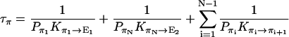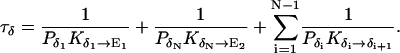1/τ_ρ corresponds to the rate of spontaneous reorientation of the water chain in equilibrium; 1/τ_π and 1/τ_δ correspond to the rates of spontaneous transfer of an excess proton and a hole from one side to the other side of the channel, respectively.

At neutral pH, a water molecule has equal probability to be protonated, i.e., to become an H₃O⁺, or deprotonated, i.e., to become an OH⁻. We assume that the translocation rate of a hole along the water chain is also the same as that of an excess proton. In this case, the two pathways E₁ ↔ π₁ ↔ ⋯ ↔ π_N ↔ E₂ and E₁ ↔ δ₁ ↔ ⋯ ↔ δ_N ↔ E₂ have the same reaction rate, i.e., τ_π = τ_δ, and Eq. 3 becomes:

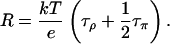(4)

τ_ρ can be obtained from the spontaneous reorientation (flipping) rate observed in the simulations. In sim0, no reorientation event was observed in the twelve CNTs during 10 ns. Therefore, τ_ρ should be at least of the order of 100 ns. We assume τ_ρ ∼ 200 ns = 2 × 10⁻⁷ s in this study. A much faster flipping rate (one per 2–3 ns) was observed in a single CNT during a 66-ns simulation (Hummer et al., 2001), corresponding to a smaller τ_ρ. We note that in the mentioned study, the single CNT was immersed in bulk water, whereas in our simulations, the CNTs formed a tightly packed bundle which partitions bulk water into two layers separated by a 15-Å water-free layer. For comparison, we also built a system of a single CNT immersed in bulk water as in Hummer et al. (2001), and indeed observed one reorientation event in a 10-ns simulation on this system. Despite the uncertainty in the flipping rate, even if our large τ_ρ value is adopted, τ_ρ, as will be shown below, is still negligible when compared with τ_π. Therefore, the choice of τ_ρ will not have a large effect on the calculated resistance of nt0.

To calculate τ_π, we need to estimate the probability P_i of each state i and the transition rate K_i→j between adjacent states i and j. In equilibrium, E₁ and E₂ are by far the most populated states, so we have 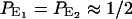. Previous studies have shown that an excess proton can hop through the water chain requiring little activation energy (Pomès and Roux, 1998). Therefore we assume that each water molecule in the CNT has the same probability (P_prot) to be protonated, i.e.,

(5)

We further assume that P_prot is the same as the probability of a bulk water molecule to be protonated. At neutral pH, the concentrations of H₃O⁺ and H₂O are 10⁻⁷ M and 55.5 M, respectively, so P_prot = 10⁻⁷/55.5 ≈ 2 × 10⁻⁹.

The activationless nature of proton hops also implies that the transition rates are all close in value, and we assume that they all have the same value K_hop. We further assume that the transition rates and are also identical to K_hop, which means that a protonated water molecule (H₃O⁺) at the end of the CNT has roughly equal probability to pass the excess proton to the next water molecule in the CNT and to bulk water. Altogether, the values are

(6)

and, hence, we obtain

(7)

Previous studies showed that the translocation of an excess proton over the entire length of the water chain occurs within ∼1 ps (Pomès and Roux, 1998). We assume accordingly that K_hop/N ∼ 1/ps = 10¹²/s, resulting in τ_π ∼ 5 × 10⁻⁴ s.

Our estimate for τ_π is three orders-of-magnitude larger than τ_ρ, so τ_ρ can be neglected in Eq. 4, and the resistance of nt0 is

(8)

This value corresponds to a rate of 1 proton per 250 μs when an EMF of 26 mV is applied. Our result shows that although the translocation of an excess proton is a very fast process (K_hop is of a sub-ps timescale), due to the very low population of π_i (i.e., small P_prot), the spontaneous transfer of a proton from one side to the other side of the channel is a much rarer event compared with the spontaneous reorientation of the water chain, and thus is the rate-limiting step for proton conduction at neutral pH. Since most of the above analysis does not involve specific properties of CNTs, the conclusions for nt0 may be generalized to other nonpolar single file water channels.

Small proton conduction in ntNPN

The description of proton conduction in nt0 can also be adopted to ntNPN, as illustrated in the corresponding diagram of protonation states in Fig. 6 a. However, in this case the water molecule in the center of the CNT needs to be treated differently from the remaining water molecules. Since both of its H atoms are involved in H-bonds with adjacent water molecules, it has no inactive H atom. Therefore, we define the skeleton of this water molecule as only its O atom and represent both of its H atoms in the diagram. Furthermore, since its O atom is strongly interacting with the positive charges of the CNT, it cannot accept an excess proton, although it may donate a proton. Therefore, this central water molecule can have three configurations: XX represents an H₂O molecule; XO or OX represents an OH⁻ ion.

FIGURE 6.

(a) Symbolic diagram for water proton configurations in ntNPN. Bold fonts were used for the water molecule at the center, since its representation has different meaning than that of the other water molecules, as explained in the text. (b) The proton conduction cycle in ntNPN, with the number of faults given for each state. The symbols β, ρ, and ω represent Bjerrum, rotation, and orientation faults, respectively.

Fig. 6 b shows the key pathway for proton conduction in ntNPN. The state at the top of the figure (corresponding to the water configuration in Fig. 6 a) is the energetically most favorable state. To transfer a proton from the right to the left starting from this state, the water chain must undergo the cycle in Fig. 6 b in counterclockwise direction, which involves the following steps: first, the leftmost water molecule must lose a proton, resulting in a hole, and the hole must propagate to the central water molecule; next, the water molecules in the left half of the CNT must rotate to restore their initial orientation; then the central water molecule (now an OH⁻) must flip its remaining H atom from the right to the left side through rotation; then the water molecules in the right half of the CNT must reorient, followed by the translocation of the hole from the central water molecule to the rightmost one; finally this rightmost water molecule must accept a proton from the bulk water, the water chain returning thereby to the initial state.

To evaluate the energy of each state in the proton conduction pathway, we define three types of faults, each coming with an energy penalty. When a water molecule becomes an H₃O⁺ or OH⁻, it forms a so-called Bjerrum fault (β) (Brünger et al., 1983; Schulten and Schulten, 1985, 1986). When two adjacent water molecules do not have an H-bond in between, they are associated with a rotation fault (ρ) (Brünger et al., 1983; Schulten and Schulten, 1985, 1986). Furthermore, in ntNPN, due to the internal electrostatic field generated by the CNT, each water molecule has a favorable orientation; if adopting the opposite orientation, the water molecule forms an orientation fault (ω). In nt0, there exist faults β and ρ with significant energy penalties, but no fault ω, since there is no internal electrostatic field preferring one water orientation over the other.

The number of faults for each state is shown in Fig. 6 b, where one can see that some states are associated with three faults (either 1β + 2ω or 1β + 1ω + 1ρ). In contrast, in nt0, each state is associated with at most one fault (either β or ρ). If we assign to the faults β, ρ, and ω energies 20 kT, 8 kT, and 10 kT, respectively, and assume that the energy of faults is approximately additive, then the proton conduction pathway in ntNPN involves an energy barrier that is ∼20 kT higher than that in nt0. Therefore, ntNPN is expected to have a much lower conductivity for protons than nt0.

DISCUSSION

In this study, we demonstrated a novel approach of organizing CNTs into a hexagonally packed arrangement, which was also adopted in Kalra et al. (2003), whereas work elsewhere consists primarily of either single free-floating or fixed CNTs. Our arrangement prevents large movements of the CNTs, and creates a two-dimensional barrier for conduction. Our approach may be useful to researchers in further studies.

Single-walled CNTs have delocalized π-electrons and exhibit semiconducting or metallic electrical conduction (Dresselhaus et al., 1996). An external electric field can alter the electronic structure of a CNT and, hence, induce a nonzero charge distribution in the CNT wall. Therefore, even though pristine CNTs are electrically neutral, they can interact with other charged atoms through field-induced polarization. However, such polarization has not been accounted for in our present simulations. While our current approach could serve the purpose of modeling biological channels, it may not accurately describe the interaction between CNT and water. An improved force field that takes into account the polarizability of CNTs is desirable in future modeling. The choice of water model (Guillot, 2002) is also worth further investigation.

AQP channels adopt a bipolar water orientation which is held responsible for proton blockage (Tajkhorshid et al., 2002). We have demonstrated that a bipolar water orientation can be reproduced in a simple model CNT (ntNPN) and conclude that ntNPN like AQPs also blocks proton conduction. We have demonstrated, through a network thermodynamic description of proton conduction, that this is indeed the case. Our description assigns a high activation barrier to the proton conduction process in ntNPN. However, we observed low water conduction in ntNPN. Fortunately, ntPNP appears to function better in this respect. ntPNP has the opposite charge distribution as ntNPN, and, therefore, its water orientations are opposite to those in ntNPN (see Fig. 4), implying that they also effectively block proton conduction.

Water conduction is two orders-of-magnitude higher in ntPNP than in ntNPN. Apparently the water molecule in the center of ntNPN has very high affinity to the two positively-charged carbon atoms, which significantly reduces the mobility of the water chain in the CNT. Similar positive charges also exist in AQP channels, including the NH₂ groups of two Asn residues and the side chain of an Arg residue (Fu et al., 2000; Murata et al., 2000; Sui et al., 2001). However, AQPs permit fast water diffusion, which may be partly due to the conformational fluctuation of the protein. In general, it is not yet clear how water diffusion and permeation in narrow water pores are quantitatively related to their geometry and charge distribution. In view of this, CNTs with different diameters (Noon et al., 2002), lengths, and charge distributions and their effect on water conduction are worth further investigation, which may shed light on the determinants of water and proton conduction rates in biological water channels.

In addition to serving as models for biological channels, different types of CNTs may also lead to technical applications. For example, chemically-modified CNTs may be designed for various capabilities, such as controlling water orientation or selectively permeating ions or protons. CNTs with high water permeation, but no ion conduction, could be used for desalination of sea water, where a hydrostatic pressure can be applied to push water through the CNTs with salt (ions) left behind.

APPENDIX

In narrow water channels such as CNTs or AQPs, water molecules form a single file and their movement is highly correlated. Single file diffusion has been extensively studied in the past, e.g., in Vasenkov and Kärger (2002). Recently, a continuous-time random-walk model (Berezhkovskii and Hummer, 2002) was proposed to describe the water movement in single-file water channels. In the following, we will briefly introduce this model, and based on it calculate the number of permeation events using an intuitive method.

In the continuous-time random-walk model (Berezhkovskii and Hummer, 2002), the channel is always occupied by N water molecules in single file. They move concertedly and cannot pass each other, i.e., exchange positions, inside the channel. The water chain moves in hops (translocations by a distance of exactly one water molecule). In equilibrium, the leftward and rightward hopping rates are the same, denoted as k₀, and the bidirectional hopping rate k is 2k₀.

A rightward permeation event is defined as a water molecule entering the channel from the left reservoir and exiting to the right reservoir. A leftward permeation event is defined similarly. The moment at which the water molecule exits the channel is taken as the time for a permeation event. The number of permeation events is often used to quantify water conduction through channels by diffusion in MD simulations (de Groot and Grubmüller, 2001; Tajkhorshid et al., 2002). This number can be predicted by the continuous-time random-walk model, as described in Berezhkovskii and Hummer (2002). Here, we give an alternative derivation.

As shown in Fig. 7, at any time, there exists a boundary in the channel which separates the i water molecules which had entered the channel from the left reservoir and the N − i water molecules coming from the right reservoir. We define such configuration as state i. At any moment, the configuration is in one of the N + 1 states, from state 0 to state N. When a leftward hop occurs, a state i will transit to state i − 1 (see Fig. 7), except for i = 0, in which case a leftward permeation event leaves the system in state 0. Similar transitions will happen for rightward hops.

FIGURE 7.

An illustration of the different permeation states as defined in Appendix. Water molecules from the left and right reservoirs are represented in blue and red, respectively.

Since the transition rate from state i to state i + 1 is the same as that from state i + 1 to i, in equilibrium, these two states should have the same probability (or same population for an ensemble) as a result of detailed balance. Therefore, the probabilities of all of the N + 1 states are the same, namely, 1/(N + 1). The number of leftward permeation events per unit time is equal to the leftward hopping rate × the probability of the occurrence of state 0, k₀/(N + 1). The number of rightward permeation events is also k₀/(N + 1). Therefore, the number p of bidirectional permeation events per unit time is

(A1)

which is the same expression as derived in Berezhkovskii and Hummer (2002).

It is noteworthy that after a permeation event, the water configuration stays in state 0 or state N, which has a relatively high probability for another permeation event in the same direction to happen. Therefore, although the leftward and rightward hops are uncorrelated, the permeation events are expected to cluster in time. Indeed, clusters of unidirectional pulses of permeation events were observed in Berezhkovskii and Hummer (2002) and Hummer et al. (2001).

References

- Berezhkovskii, A., and G. Hummer. 2002. Single-file transport of water molecules through a carbon nanotube. Phys. Rev. Lett. 89:064503. [DOI] [PubMed] [Google Scholar]
- Borgnia, M., S. Nielsen, A. Engel, and P. Agre. 1999. Cellular and molecular biology of the aquaporin water channels. Annu. Rev. Biochem. 68:425–458. [DOI] [PubMed] [Google Scholar]
- Branden, C., and J. Tooze. 1991. Introduction to Protein Structure. Garland Publishing, New York and London.
- Brünger, A., Z. Schulten, and K. Schulten. 1983. A network thermodynamic investigation of stationary and non-stationary proton transport through proteins. Z. Phys. Chem. NF136:1–63. [Google Scholar]
- de Groot, B. L., and H. Grubmüller. 2001. Water permeation across biological membranes: mechanism and dynamics of aquaporin-1 and GlpF. Science. 294:2353–2357. [DOI] [PubMed] [Google Scholar]
- Dresselhaus, M. S., G. Dresselhaus, and P. C. Eklund. 1996. Science of Fullerenes and Carbon Nanotubes. Academic Press, San Diego, CA.
- Essmann, U., L. Perera, M. L. Berkowitz, T. Darden, H. Lee, and L. G. Pedersen. 1995. A smooth particle mesh Ewald method. J. Chem. Phys. 103:8577–8593. [Google Scholar]
- Fu, D., A. Libson, L. J. W. Miercke, C. Weitzman, P. Nollert, J. Krucinski, and R. M. Stroud. 2000. Structure of a glycerol conducting channel and the basis for its selectivity. Science. 290:481–486. [DOI] [PubMed] [Google Scholar]
- Guillot, B. 2002. A reappraisal of what we have learnt during three decades of computer simulations on water. J. Mol. Liq. 101:219–260. [Google Scholar]
- Hummer, G., J. C. Rasaiah, and J. P. Noworyta. 2001. Water conduction through the hydrophobic channel of a carbon nanotube. Nature. 414:188–190. [DOI] [PubMed] [Google Scholar]
- Humphrey, W., A. Dalke, and K. Schulten. 1996. VMD—Visual molecular dynamics. J. Mol. Graph. 14:33–38. [DOI] [PubMed] [Google Scholar]
- Iijima, S. 1991. Helical microtubules of graphitic carbon. Nature. 354:56–58. [Google Scholar]
- Jorgensen, W. L., J. Chandrasekhar, J. D. Madura, R. W. Impey, and M. L. Klein. 1983. Comparison of simple potential functions for simulating liquid water. J. Chem. Phys. 79:926–935. [Google Scholar]
- Kalé, L., R. Skeel, M. Bhandarkar, R. Brunner, A. Gursoy, N. Krawetz, J. Phillips, A. Shinozaki, K. Varadarajan, and K. Schulten. 1999. NAMD2: greater scalability for parallel molecular dynamics. J. Comp. Phys. 151:283–312. [Google Scholar]
- Kalra, A., S. Garde, and G. Hummer. 2003. Osmotic water transport through carbon nanotube arrays. Proc. Natl. Acad. Sci. USA. In press. [DOI] [PMC free article] [PubMed]
- MacKerell, A. D., Jr., D. Bashford, M. Bellott, R. L. Dunbrack, Jr., J. D. Evanseck, M. J. Field, S. Fischer, J. Gao, H. Guo, S. Ha, D. Joseph, L. Kuchnir, K. Kuczera, F. T. K. Lau, C. Mattos, S. Michnick, T. Ngo, D. T. Nguyen, B. Prodhom, W. E. Reiher III, B. Roux, M. Schlenkrich, J. Smith, R. Stote, J. Straub, M. Watanabe, J. Wiorkiewicz-Kuczera, D. Yin, and M. Karplus. 1998. All-hydrogen empirical potential for molecular modeling and dynamics studies of proteins using the CHARMM22 force field. J. Phys. Chem. B. 102:3586–3616. [DOI] [PubMed] [Google Scholar]
- Miller, S. A., V. Y. Young, and C. R. Martin. 2001. Electroosmotic flow in template-prepared carbon nanotube membranes. J. Am. Chem. Soc. 123:12335–12342. [DOI] [PubMed] [Google Scholar]
- Murata, K., K. Mitsuoka, T. Hirai, T. Walz, P. Agre, J. B. Heymann, A. Engel, and Y. Fujiyoshi. 2000. Structural determinants of water permeation through aquaporin-1. Nature. 407:599–605. [DOI] [PubMed] [Google Scholar]
- Noon, W. H., K. D. Ausman, R. E. Smalley, and J. Ma. 2002. Helical ice-sheets inside carbon nanotubes in the physiological condition. Chem. Phys. Lett. 355:445–448. [Google Scholar]
- O'Connell, M. J., S. M. Bachilo, C. B. Huffman, V. C. Moore, M. S. Strano, E. H. Haroz, K. L. Rialon, P. J. Boul, W. H. Noon, C. Kittrell, J. Ma, R. H. Hauge, R. B. Weisman, and R. E. Smalley. 2002. Band gap fluorescence from individual single-walled carbon nanotubes. Science. 297:593–596. [DOI] [PubMed] [Google Scholar]
- Pomès, R., and B. Roux. 1998. Free energy profiles for H+ conduction along hydrogen-bonded chains of water molecules. Biophys. J. 75:33–40. [DOI] [PMC free article] [PubMed] [Google Scholar]
- Pomès, R., and B. Roux. 2002. Molecular mechanism of H+ conduction in the single-file water chain of the gramicidin channel. Biophys. J. 82:2304–2316. [DOI] [PMC free article] [PubMed] [Google Scholar]
- Schulten, Z., and K. Schulten. 1985. Model for the resistance of the proton channel formed by the proteolipid of ATPase. Eur. Biophys. J. 11:149–155. [DOI] [PubMed] [Google Scholar]
- Schulten, Z., and K. Schulten. 1986. Proton conduction through proteins: an overview of theoretical principles and applications. Meth. Enzym. 127:419–438. [DOI] [PubMed] [Google Scholar]
- Sui, H., B.-G. Han, J. K. Lee, P. Walian, and B. K. Jap. 2001. Structural basis of water-specific transport through the AQP1 water channel. Nature. 414:872–878. [DOI] [PubMed] [Google Scholar]
- Tajkhorshid, E., P. Nollert, M. Ø. Jensen, L. J. W. Miercke, J. O'Connell, R. M. Stroud, and K. Schulten. 2002. Control of the selectivity of the aquaporin water channel family by global orientational tuning. Science. 296:525–530. [DOI] [PubMed] [Google Scholar]
- Vasenkov, S., and J. Kärger. 2002. Different time regimes of tracer exchange in single-file systems. Phys. Rev. E. 66:052601. [DOI] [PubMed] [Google Scholar]
- Wind, S. J., J. Appenzeller, R. Martel, V. Derycke, and P. Avouris. 2002. Vertical scaling of carbon nanotube field-effect transistors using top gate electrodes. Appl. Phys. Lett. 80:3817–3819. [Google Scholar]