Solid Phase DNA Amplification: A Simple Monte Carlo Lattice Model

Abstract

Recently, a new way to amplify DNA, called solid phase amplification (SPA), has been introduced. SPA differs from the traditional polymerase chain reaction (PCR) in the use of surface-bound instead of freely-diffusing primers to amplify DNA. This limits the amplification to two-dimensional surfaces and therefore allows the easy parallelization of DNA amplification in a single system. Furthermore, SPA could provide an alternate route to DNA target implantation on DNA chips for genomic studies. Standard PCR processes are usually characterized (at least initially) by an exponential growth and a broad population distribution, and they are well described by the theory of branching processes, wherein a generating function can be used to obtain the probability distribution function for the population of offspring. This theoretical approach is not appropriate for SPA because it cannot properly take into account the many-body (steric) and geometric effects in a quenched two-dimensional environment. In this article, we propose a simple Lattice Monte Carlo technique to model SPA. We study the growth, stability, and morphology of isolated DNA colonies under various conditions. Our results indicate that, in most cases, SPA is characterized by a geometric growth and a rather sharp size distribution. Various non-ideal effects are studied, and we demonstrate that such effects do not generally change the nature of the process, except in extreme cases.

INTRODUCTION

Since its invention in 1983, the polymerase chain reaction (PCR) has transformed molecular biology by allowing researchers to make unlimited copies of a single DNA fragment in a matter of hours. PCR is usually performed by first mixing the necessary components in a vial. The amplification then takes place in all of the available volume. Usually, only one target sequence is amplified for each PCR experiment. This means that if different DNA strands are amplified simultaneously (i.e., Multiplex PCR), they have to be separated afterward (using, for example, gel electrophoresis; see Pang et al., 2002). Recently, a new type of DNA amplification, called solid phase amplification (SPA), has been introduced by two different groups: Adessi et al. (2000) and Bing et al. (1996). By attaching the primers to a solid surface, SPA allows an amplification limited to a well-defined two-dimensional area. Since it results in a spatially located amplification, it is possible to amplify a large number of different DNA strands in the same experiment (i.e., onto the same solid surface) without mixing them. This characteristic could be very useful for the design of DNA chips.

It is common to make use of the theory of branching processes to model PCR (Peccoud and Jacob, 1996). In this framework, a generating function provides the probability distribution function for the number of offspring, given the initial number of molecules and the total number of PCR cycles. However, the theory of branching processes is not appropriate in the case of SPA because it cannot take into account the many-body interactions in a quenched environment such as molecular crowding (a chain has less chance to produce an offspring when surrounded by other chains). Furthermore, such theories cannot provide any spatial or density information. In this article, we propose a simple approach to modeling SPA. We reduce the system to a lattice model where a given site can be either occupied by one DNA molecule or left empty. Monte Carlo techniques are then used to simulate the amplification process, i.e., the growth of the colony. The model is thus reminiscent of the models used for the growth of tumors and bacterial colonies (Eden, 1961; Meinhardt, 1982; Sams et al., 1997; Wagner et al., 1999; Williams and Bjerknes, 1972; Ziqin and Boquan, 1995).

This article is organized as follows. The next section describes and explains the PCR process and reviews the standard way to model PCR, the branching process theory. The following two sections then introduce the new technique of solid phase DNA amplification and our Monte Carlo lattice model and results, respectively. We end with our discussion and conclusions.

SOLUTION PCR

PCR is based on the activity of polymerase, a naturally occurring enzyme that acts on a single stranded DNA fragment (ssDNA) and generates its complementary strand. Two characteristics of polymerase make PCR possible. First, polymerase cannot copy a DNA chain without a short sequence of nucleotides to “prime” the process, i.e., to get the process started. This initial stretch of DNA is called a primer. The primers are generated synthetically and are designed to complement a specific sequence at one end of the target sequence (the section of the DNA fragment that needs to be amplified). The other essential characteristic of polymerase is that it can only act on one end (the 3′-end) of the primer. This comes from the structure of the sugar molecules used in the DNA double helix. In a PCR experiment, two primers are usually required (one for each strand). By carefully choosing these two primers, it is possible to multiply a selected section of the total DNA fragment: only the section contained between the two primers (the target sequence) is then amplified (Fig. 1).

FIGURE 1.

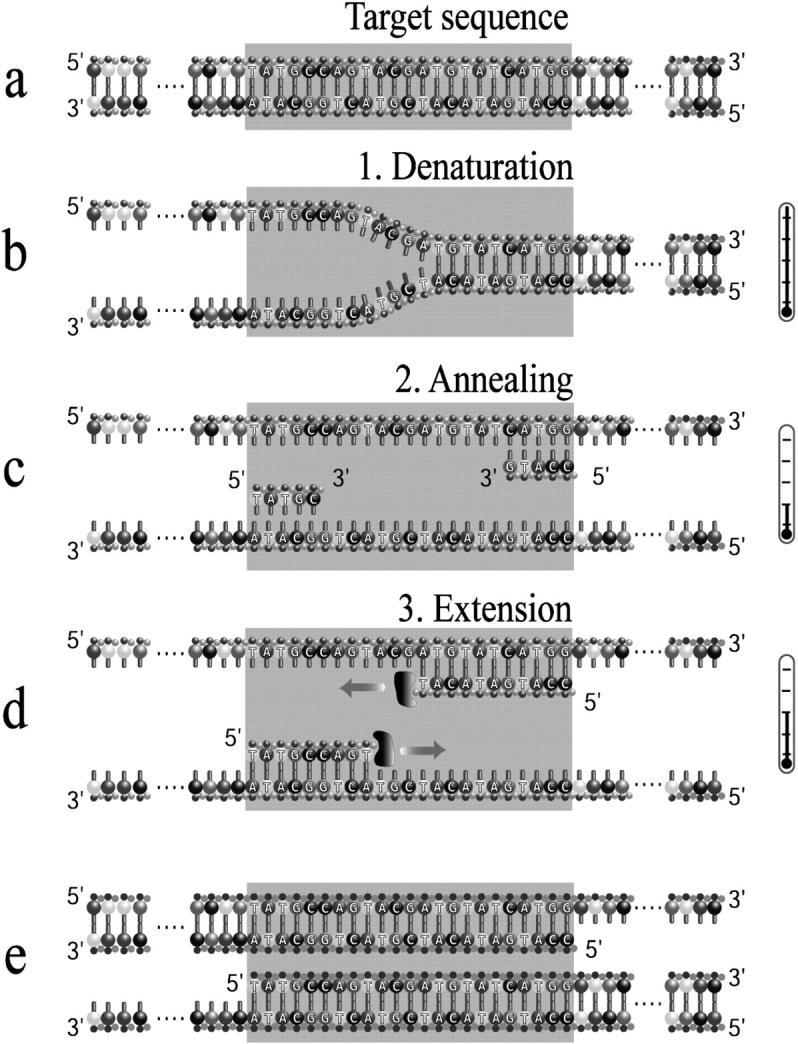
Representation of the PCR process. A dsDNA fragment is first heated (a) to break the molecule into its two complementary fragments (b). The solution is then cooled down to allow the primers to bind to their complementary sequences along the DNA fragments (c). Finally the solution is reheated to allow the polymerase to add nucleotides at the end of the primers and eventually make a complementary copy of the template (d). Because the polymerase can only act on one end of the DNA (the 3′ end), the solution quickly consists almost exclusively of DNA fragments corresponding to the target sequence located between the two selected primers (e).

In a typical PCR experiment, the four necessary components—piece(s) of DNA, large quantities of the four nucleotides (adenine A, cytosine C, guanine G, and thymine T), large quantities of the two primers, and DNA polymerases—are mixed in an aqueous solution (the buffer, which is also used to maintain proper pH and salt concentrations). The PCR process itself usually consists of sequentially heating (to denature the double-stranded DNA), cooling down (to allow the primers to hybridize to the ssDNA fragments) and reheating the mixture (to allow the polymerase to complete the double helix). Those three steps are respectively called denaturation, annealing, and extension (see Fig. 1). After a few cycles, exact replicas of the target sequence have been produced. In the subsequent cycles, dsDNA of both the original molecules and the copies are used as templates. Solution PCR is thus characterized, at least initially (after a while, a lack of nucleotide and/or primer and/or enzyme can affect the growth rate), by an exponential growth. After several cycles, the pool is greatly enriched in pieces of DNA containing the target sequence. In ∼1 h, as many as n = 25 cycles can be completed, giving up to a 2²⁵ ≃ 67-million-fold increase in the amount of the target sequence.

In practice, however, PCR amplification is not perfect. For example, a PCR thermal cycle can finish before the polymerase has completely copied the DNA. The copy is then said to be a sterile molecule and it is unable to replicate in the following cycle. It is also possible that the molecule simply does not find a matching primer in the annealing phase. These phenomena slow down the growth of the population size. Therefore, the expected population grows like ∼yⁿ, with y < 2 (typically y ≃ 1.9; see Bing et al., 1996).

Nonspecific hybridization of the primer can also occur and can lead to the amplification of nonspecific PCR products. The case of a primer using the other primer as a template leads to the formation of primer-dimers (Brownie et al., 1997; Halford et al., 1999; Hogdall et al., 1999; Markoulatos et al., 2002; Nazarenko et al., 2002; Wabuyele and Soper, 2001). Because they contain both primer annealing sites, primer-dimers are valid templates and are amplified very efficiently. They may even become the predominant PCR product. To avoid mis-hybridization and the formation of primer-dimers, great care must be taken in the primer design and in the choice of experimental conditions. For example, too short a primer (primer lengths of 18–30 bases are optimal for most PCR applications), complementarity among the 3′ ends of the two primers, low annealing temperatures, high enzyme concentrations, and high primer concentrations have all been shown to increase the frequency of primer-dimer formation (Brownie et al., 1997; Markoulatos et al., 2002).

As previously mentioned, solution PCR leads, at least initially, to an exponential amplification of the target sequence. This is due to the fact that every molecule (the original ones as well as the copies) can be duplicated at each cycle. Solution PCR is thus characterized by the yield of the reaction, p, which is the probability that a DNA molecule produces a fertile copy during a cycle. The growth remains exponential as long as p stays constant. It is the case for the first cycles because PCR is usually carried out with a large excess of reagents (nucleotides, primers, and polymerases) such that the DNA molecules do not have to compete to copy themselves. After a while (typically 20 cycles), however, there are not enough reagents to satisfy all the DNA targets, and both the reaction yield p and the growth rate decrease.

Unless the reaction yield p is equal to 1 or 0, PCR is a random process. If we start with a single copy of the target, the population could be anywhere between 1 and 2ⁿ after n amplification cycles. To simulate this amplification, a simple Monte Carlo procedure can obviously be useful. However, since PCR is intrinsically a simple discrete process, branching theory can also be used (Peccoud and Jacob, 1996). This straightforward, yet powerful theory allows one to quickly obtain the mean value of the DNA population and the probability distribution of offspring using a generating function.

In the framework of the branching process theory, the discrete growth of a population is written in terms of the generating function (Bailey, 1963; Feller, 1968):

(1)

where p_k is the probability that one molecule gives rise to k molecules after one generation (i.e., after one PCR cycle in our case). The probability distribution for the population after n generations is given by the composition of the generating function over itself n times:

(2)

where the coefficient of the s^k term is then the probability of having k molecules after n generations. Using this iterative approach, it is possible to obtain the exact probability distribution function for the population after n generations.

If the process is started with just one individual (m₀ = 1), the expected population size after n generations, M_n, is given by Bailey (1963) and Feller (1968) as

(3)

In the case of a larger initial number of molecules (m₀ > 1), each of them will, independently, give rise to a branching process. The probability-generating function for the n^th generation would thus be Therefore, the expected population size after n generations is M_n = m₀ × (P′(1))ⁿ and the probability distribution function tends toward a Gaussian form when the initial copy number m₀ is increased (Feller, 1968).

During a PCR cycle, a molecule can either duplicate or not. The probabilities associated with those events are respectively denoted as p and 1 − p. Therefore the generating function of a PCR cycle is reduced to

(4)

The expected DNA population of a PCR amplification experiment starting with a single molecule is thus given by

(5)

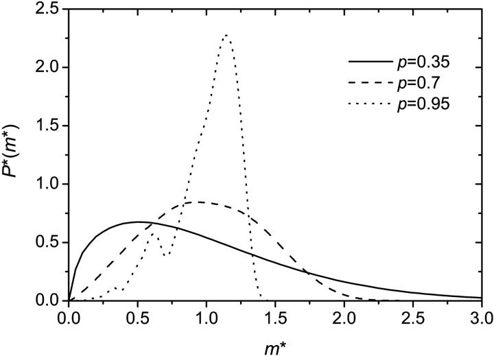
Using Eq. 2, it is possible to obtain the probability distribution function for the DNA population for arbitrary values of p. Fig. 2 shows three samples distributions obtained after n = 10 iterations. The population sizes (the x-axis) m_n were divided by the expected value (m^* = m_n/M_n) to make comparisons easier. The general shape of the distribution is almost independent of the number of cycles for n ≥ n^* ≃ 10. In general, we see that the larger the value of p, the sharper the distribution. Also, for large values of p (p ≥ p^* ≃ 0.82), the distribution is actually multimodal. This is due to the fact that the initial amplification is then critical: a failure of the original molecule to duplicate in the first cycle has a lasting impact. For large values of p, the distribution thus contains (at least) two peaks: one corresponding to the case where the initial amplification failed, and the other one (the larger one) where it was successful. As the amplification yield p approaches its maximum value (p = 1), other peaks progressively appear corresponding to the cases where one of the molecules failed to reproduce in the second cycle, then in the third cycle, and so on.

FIGURE 2.

Probability distribution of the DNA population for different PCR amplification yields p (using n = 10). For the distribution is multimodal. The x-axis is the normalized (so the expected value is 1 for all p) size of the population (M^* = m₁₀/M₁₀) whereas the y-axis is the probability multiplied by the expected population size P^*(M^*) = M₁₀P₁₀(M^*). The general shape of the distribution is almost completely independent of the number of cycles for n ≥ n^* = 10. The distributions were obtained starting with a single initial molecule. The distribution tends to become Gaussian when the initial copy number is increased.

PCR is often used to detect substances that are present in very small concentrations (e.g., viral DNA). It is highly effective if one only wants to know if a given substance is present or not. A harder task is quantitative PCR (Q-PCR) where one's goal is to determine the initial number of molecules (m₀), given the final population (m_n) of a single experiment, the (estimated) amplification yield p, and the number of PCR cycles (n) (Boom et al., 2002; He et al., 2002; Stevens et al., 2002). Fig. 2 shows why Q-PCR is difficult in practice. When the amplification yield p is small, the probability distribution is broad and has a large standard deviation. On the other hand, when p is large, the distribution is multimodal. Note that Fig. 2 represents the extreme case where the initial number of molecules is 1. The situation is less critical when m₀ is larger. However, it is precisely when the number of initial molecules is very small and cannot be directly detected using other methods that PCR should be used! Furthermore, the final number of molecules is only known approximately and it is very hard to have a reliable value for the amplification yield p. Nevertheless, Q-PCR has been shown to be useful. It is used, for example, to provide an estimate of the virus load during HIV and hepatic infections (Boom et al., 2002; Stevens et al., 2002).

SOLID PHASE AMPLIFICATION

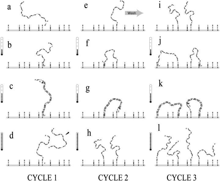
The central idea of this novel method is to attach the 5′-end of the primers to a surface (silica, polystyrene bead, …) instead of letting the primers freely diffuse in a bulk solution (see Fig. 3 a) (Adessi et al., 2000; Bing et al., 1996). The primers then form a very dense carpet (the density is ∼10¹¹ primers per mm²—Adessi et al., 2000—which corresponds to a mean distance of the order of ∼5–10 nm between primers; note that this is similar to the contour length of a primer). In this context, the amplification can occur via two processes. First, a freely diffusing DNA target can be captured on the surface and then copied by the polymerase (see Fig. 3, a–d). This is called interfacial amplification. Note that the copy stays attached to the surface whereas the initial DNA molecule returns to the solution after the annealing step. After several DNA copies are attached to the surface via interfacial amplification, a second type of amplification can take place. In this case, the free end of the attached copy hybridizes to the primer (attached to the surface) complementary to its sequence, and the amplification process can start (see Fig. 3, e–l). It is important to note that this surface amplification process leaves both molecules attached to the surface, hence its name. Therefore, solid phase DNA amplification leads to the growth of a colony of molecules attached to the surface and located in the same region. This characteristic could easily be exploited in the design of DNA microarrays.

FIGURE 3.

Representation of the solid phase amplification process. In the first cycle (a-b-c-d) the DNA is replicated by the interfacial amplification. The net result is that one ssDNA is now attached to the surface via the primer. The solution is then changed with a new one free of DNA targets. In the following cycles (e-f-g-h and i-j-k-l), only surface amplification is possible. This results in a spatially located DNA colony. Note that since a molecule always generates its complementary sequence in a thermal cycle, the two complementary branches will be present in the colony and two different types of primers have to be attached to the surface.

The procedure for solid phase amplification can be separated in three distinct steps—annealing, extension, and denaturation—which are repeated in an iterative way. In the first cycle, interfacial amplification is the only type of amplification possible. The result of the first cycle is thus to obtain a certain number of target DNAs attached to the surface via the primers. In subsequent cycles, surface amplification is also possible since some of the target DNAs are now attached to the surface. However, when the two types of amplification process coexist, interfacial amplification is usually predominant (Adessi et al., 2000). Therefore, to obtain surface amplification, the initial solution has to be washed away and replaced with a solution free of DNA targets. Surface amplification is then the only amplification possible and the temperature cycles can be started again. The net result of a surface amplification event is to obtain a new ssDNA molecule attached to the surface in the immediate proximity of the initial strand (Fig. 3, h–i). Note that the length of the molecules used in SPA is typically 400 bases (contour length of ∼170 nm). The radius of gyration in the hybridization phase (ssDNA) is thus ∼15–20 nm which is larger than the mean distance between nearest-neighbor primers (∼5–10 nm). Also, a typical DNA length is much larger than the persistent length of ssDNA (∼10 bases or ∼4 nm) but is similar to that of dsDNA (∼150 basepairs or ∼51 nm). Therefore, the molecule is very flexible in the hybridization phase, and has no problem bending to find matching primers. However, at the end of the elongation phase (when the molecule is completely double-stranded), it becomes quite rigid and must be under considerable bending stress.

Surface amplification results in an area covered with copies of both strands of the original DNA target. This can be seen as a DNA colony. The number of colonies depends on the number of DNA targets captured (via interfacial amplification) before the initial solution is washed. If different DNA targets are captured, many types of colonies will exist on the surface.

Two strategies can be used for primer implantation. Specific primers can be used so that the hybridization (and the amplification) is only possible for a specific DNA target. A chip can then be designed so that each sub-area is specific for one target, and it is possible to detect target sequences without using solution-based primer sets, hybridization, or electrophoresis (Bing et al., 1996). Another approach consists of adding, at both ends of the nucleic acid templates to be analyzed, the linker sequences complementary to the immobilized primers (Adessi et al., 2000). In this case, it is possible to amplify each template molecule irrespective of their actual sequence. Note that the colonies are then randomly arrayed. If the colonies are far enough from each other (favored by using a small concentration of DNA targets in the initial solution), each colony is amplified but remains isolated from the others (no merging occurs between neighboring colonies). SPA thus allows the parallelization of the DNA amplification process without any direct human intervention. In both scenarios, the actual growth of the colonies is similar.

The process described in Fig. 3 corresponds to the ideal case in which the primer cannot be removed from the surface. In reality, the successive heating and cooling of the solution can cause the primer to detach from the surface. A recent study (Adessi et al., 2000) showed that, even in the most suitable case, up to 50% of the primers had detached after 28 cycles. Of course, the primers can also detach after a DNA target has been “attached” to it. Therefore, after a couple of cycles, the solution can contain some free diffusing targets and primers. In this context, solution PCR followed by interfacial amplification is still possible in principle. However, experimental work (Adessi et al., 2000) showed that this process is negligible, perhaps because of the very small concentration of DNA targets and primers present in solution. It is also possible to avoid solution PCR completely by changing the chemical mix at each cycle.

The number of molecules in a given SPA colony does not increase exponentially (with the exception of the first few cycles) as in the case for solution PCR. The reason is molecular crowding. Two free molecules separated by less then their radius of gyration (R_g) will interact sterically with each other, and will tend to repulse each other. In SPA, a duplicated molecule (child), will always be in the vicinity of the original molecule (parent). Therefore, the parent molecule will not be able to bend and make a new molecule in the vicinity of its child and vice versa. When a molecule is completely surrounded by others, its free end tends to move away form the surface (like in a dense polymer brush; Currie et al., 2000; Netz and Schick, 1998; Skvortsov et al., 1999). Therefore, after a few cycles, a molecule at the center of the colony (which is thus surrounded by others) will have a smaller duplication probability (its free end is less likely to find a matching primer on the surface). Because of this phenomenon, a DNA colony should be characterized by a roughly constant density and should grow outwards, i.e., from its perimeter. Since only the perimeter can reproduce freely, the growth cannot be exponential.

Like in solution PCR, a SPA cycle can finish before the polymerase has completely copied the DNA, resulting in a sterile molecule. In solution PCR, this simply reduces the growth rate of the amplification. In SPA the impact can be more severe because the sterile molecule is attached to the surface and will interact sterically with its neighbor. When the edge of the colony is obstructed by sterile molecules, the latter can act as a fence and slow down, or even stop, the growth of the colony. Note that there is a certain (small) probability for a sterile molecule to become fertile again in subsequent cycles (the sterile molecule may rehybridize to a fertile molecule, allowing the polymerase to complete its DNA sequence).

SIMULATING SOLID PHASE AMPLIFICATION

As mentioned previously, the branching process theory is not appropriate for solid phase DNA amplification because it is based on the assumption that the amplification yield is the same for all molecules and remains unchanged over all cycles. Although somewhat realistic in the case of solution PCR, those assumptions are obviously not valid for SPA because of the many-body (steric) interactions (see Solution PCR). In this section, we propose a simple lattice Monte Carlo system to model SPA and we present simulation results.

The simplest possible system, where a molecule can only create a copy of itself on an empty lattice site immediately adjacent to its position (with a probability 0 < p ≤ 1), is considered in The Basic System. In the following subsections, the model is generalized to include sterile molecules (Sterilization) and molecules detaching from the surface (Detachment). In The Colony Density Profile, the model is further generalized to allow a greater density at the center of the colony. To do so, two alternatives are explored (adding a probability for a molecule to generate a copy of itself in between existing molecules and allowing more than one molecule to occupy each site of the lattice). In each case, the growth of the colony is examined as well as its stability and morphology.

As we shall see, a realistic representation of a SPA experiment must include many parameters. Also, while a lattice representation greatly simplifies the simulation, some important choices are still necessary regarding the algorithm itself. Choosing a good algorithm and a good set of parameters likely requires a combination of precise experimental data and microscopic simulations, e.g., detailed and extensive molecular dynamics or Brownian dynamics simulations of realistic chains attached to surfaces. Instead of trying all possible options and sets of parameters, educated guesses are made, allowing an overview of the possibilities and an understanding of the general phenomenon of SPA. Therefore, this work should not be seen as a final product, but rather as a starting point, aiming at guiding what needs to be done experimentally and in terms of microscopic simulations.

The basic system

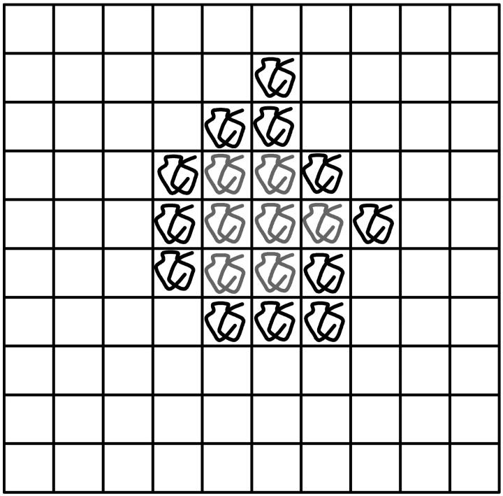
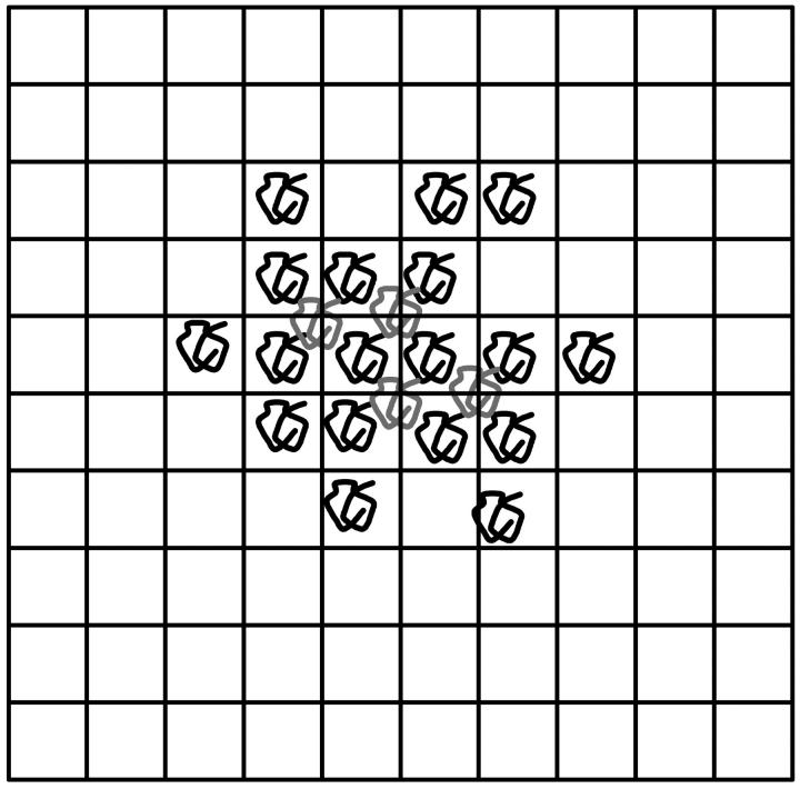
The simplest way to model SPA is to use a lattice algorithm where each site can be either occupied by a ssDNA molecule or left empty (an empty site is actually occupied by several primers since the latter form a dense carpet). Fig. 4 shows a simple example of such a system. At each thermal cycle, a ssDNA molecule can either generate a copy on one of its empty nearest neighbor sites or stay inactive. Although very simple, this model better represents SPA than branching processes because it includes the essence of the molecular crowding phenomenon, i.e., when all the nearest neighbors of a molecule are occupied, the latter cannot produce further copies. The model thus assumes that the duplicated molecules are always roughly at the same distance from the original molecules and that once a molecule is surrounded by four others (we use a square lattice), its free end remains away from the surface so that it cannot duplicate.

FIGURE 4.

Example of an SPA representation on a square lattice system. A lattice site can be occupied by an ssDNA molecule or left empty. At each cycle, a molecule can either make a copy on one of the nearest neighbor empty sites or stay inactive. When all four nearest neighbor sites are occupied (molecules in gray), the molecule cannot produce copies anymore.

The simulation algorithm goes as follows. A molecule is first placed at the center of a square lattice. At each cycle, each molecule makes one attempt to copy itself into one of its empty nearest neighbor sites (if any). If more than one such site is available to a molecule, one of them is chosen randomly, but the molecule still has only one chance (per cycle) to make a copy. Therefore, two molecules can try to generate a copy onto the same site, but only one can be successful. Each attempt has a probability p of being successful. When a molecule is completely surrounded by others (i.e., all its nearest neighbors are occupied by other molecules), it cannot produce any more copies. Note that a colony is actually made of both strands of the original DNA target (see Solid Phase Amplification). We do not, however, distinguish between the two types.

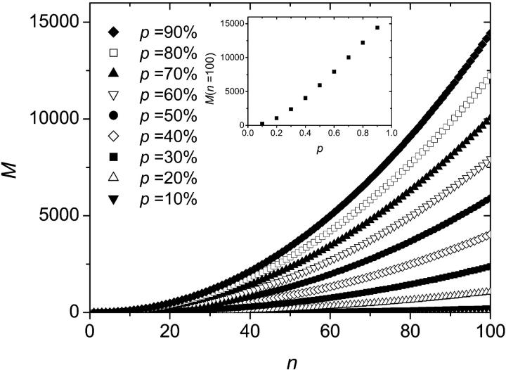
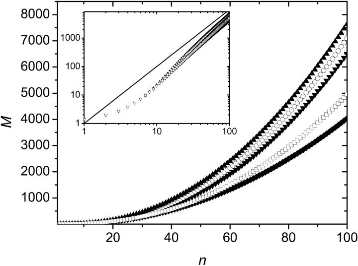
Simulations were performed for up to 100 thermal cycles and were averaged over 100,000 colonies for each set of parameters. Fig. 5 shows the average size M(n) of a colony (defined as the number of fertile molecules in the colony), as a function of the number n of thermal cycles, for various values of p (Fig. 5, inset, shows the average size of a colony after n = 100 iterations as a function of p). As expected, a larger value of p leads to a faster increase of the colony size. Also, the growth in the size of the population is slower than for solution PCR. This is so because once a molecule is surrounded by others, it stops copying itself (this is the molecular crowding issue that we mentioned previously). Therefore, apart from the very first few cycles, the colony grows mostly from its perimeter. Since the radius r of the colony increases linearly with the number n of generations,

(6)

its surface area, A(n), scales like

(7)

If we assume that most of the sites inside the colony are occupied, which is certainly the case for the “old” sites away from the colony perimeter, the colony grows in a geometrical manner:

(8)

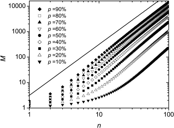
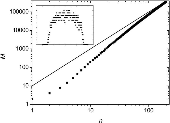
This can be verified on Fig. 6 where the evolution of the colony size (M(n)) is shown on a log-log graph. An asymptotic slope of 2 is clear for all values of p. The initial exponential growth ceases when the core of the colony reaches its maximum density of one molecule per lattice site.

FIGURE 5.

Average size M of the colony as a function of the number n of SPA cycles. Each colony starts with a single molecule. The data were averaged over 100,000 colonies for each set of parameters. A larger value of p leads to a faster increase of the colony size. Inset: Average size of a colony after n = 100 iterations as a function of p.

FIGURE 6.

Average size M of the colony as a function of the number n of SPA cycles. Apart from the very first few cycles, the relation is linear for all values of p, and for large n, the slope approaches a value of 2 (solid line). Therefore the colony grows in a geometrical manner, M(n) ∝ n².

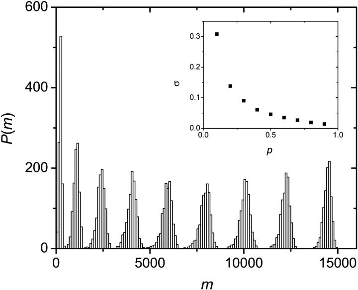
Fig. 7 shows the distribution of colony sizes for p = 10% to p = 90% with 10% intervals. The distributions are much sharper than the one obtained for solution PCR (compare to Fig. 2). This is so because solid phase amplification is less sensitive to failures in the first few thermal cycles. When normalized, the standard deviation of the distributions decreases sharply when p increases (Fig. 7, inset), as one would expect.

FIGURE 7.

Distribution of colony sizes m for p = 10% to p = 90% (from left to right) with 10% intervals. All distributions are much sharper than that obtained by solution PCR (see Fig. 2). We used ensembles of 1000 colonies and n = 1000 cycles. Inset: Normalized standard deviation as a function of p.

Sterilization

As explained in the previous section, a thermal cycle can finish before the polymerase has completely copied the DNA strand, resulting in a sterile molecule. Such a molecule is unable to produce new copies because the DNA sequence at its free end does not correspond to the primer sequences on the surface. However, a sterile molecule still occupies space; therefore, it applies steric constraints to its neighbors and can prevent them from duplicating. Note that a sterile molecule can become fertile again in subsequent cycles if it rehybridizes with a fertile molecule.

The algorithm presented in the last section was modified to account for these phenomena. First, each new molecule is now assumed to have a probability s to be born sterile (the probability to generate a sterile molecule is thus ps). Note that a sterile molecule still occupies one lattice site, and therefore prevents a fertile molecule from occupying it. We thus make the approximation that a sterile molecule, with a smaller radius of gyration, has the same steric impact as a fertile one. Second, to account for the possible rehybridization of a sterile molecule, we assume that when a fertile molecule is completely surrounded by others (all its nearest neighbors are occupied), it tries to recombine with one of its neighbors (one of the four neighbors is chosen randomly). If this neighbor happens to be sterile, it has a probability r to complete its sequence, thus rendering it fertile (we also assume that all the fertile molecules can rehybridize with a sterile molecule even though only molecules that are its complement can actually do it). Note that both s and r are assumed to be constant during the simulation, i.e., from cycle to cycle.

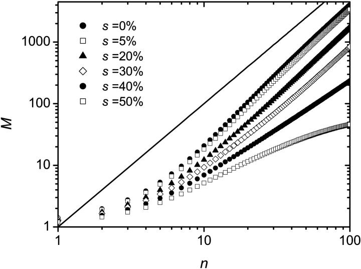
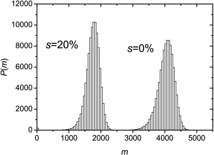
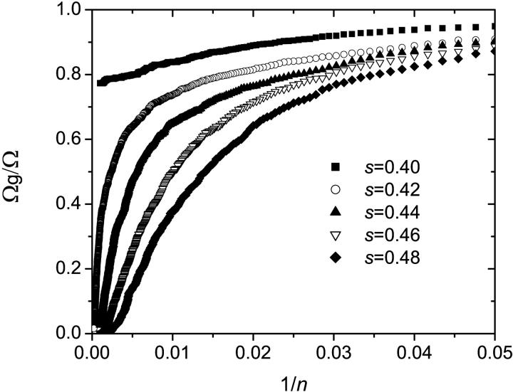
Simulations were performed using this algorithm and the recombination mechanism was first assumed to be negligible (r = 0). The probability for a molecule to make a copy was set to p = 0.4, the number of thermal cycles to n = 100 and the results were averaged over 100,000 colonies. Since a sterile molecule is unable to copy itself, a larger probability s to obtain a sterile molecule results in a slower growth. This can be seen in Fig. 8, where the number of fertile molecules is plotted as a function of the number of cycles for various values of s. When s ≠ 0%, there is a finite probability that a colony simply stops growing because all the molecules on its perimeter turn out to be sterile. In principle, this could happen at any stage of the development of the colony. In reality, however, when s < s^* ≃ 41%, the colony either stops growing after only a few cycles or grows indefinitely. As an example, the distributions of colony sizes are compared in Fig. 9 for s = 0% and s = 20%. Apart form the obvious fact that the mean colony size decreases when s increases, there is apparently little difference between the two distributions. However, we note a little bump near the origin for the s = 20% case: this corresponds to the colonies that died young. As s is increased, the probability that the colony stops growing at a later stage increases, and when s > s^* ≈ 41%, the colony is doomed to die (the average size of the colonies converges to a finite value: M(n→∞) ≠ ∞). This can be observed in Fig. 10 where the size distributions are plotted for s = 40% and s = 50%. Those critical effects can also be seen on Fig. 11 where the fraction of colonies still growing after n cycles Ωg/Ω, is plotted as a function of the inverse of the number of cycles (1/n) for different values of s. When s < s^* ≈ 41%, the number of growing colonies converges to a finite value. Another important result is that when s < s^* the growth of the colony remains geometric, i.e., we still have M ∼ n². The actual value of s^* is expected to be equal to the site percolation threshold c^* of the given lattice. For the two-dimensional square lattice, we have c^* = 0.407254 (Stauffrer and Aharony, 1992), which is compatible with our value of s^* ≈ 41%.

FIGURE 8.

Average size M of the colony (number of fertile molecules) as a function of the number n of cycles for various values of s. The solid line corresponds to a geometric growth and has a slope of 2. A sterile molecule is not able to copy itself, therefore a larger probability s to generate a sterile molecule results in a slower growth. For each set of data, the results were averaged over 100,000 colonies and p = 0.4 was used.

FIGURE 9.

Distribution of colony sizes M for s = 0% and s = 20% (p = 0.40 in both cases). Apart from the obvious fact that the mean size of the colony is larger for s = 0%, and the little bump at the beginning of the s = 20% curve (due to colonies that have stopped growing because all the molecules on their perimeter were sterile), there is little difference between the two distributions. The ensemble is made of 100,000 colonies and we allowed n = 100 cycles. We have M_0% = 4036, σ_0% = 247, and M_20% = 1745, σ_20% = 217. For s = 20%, the total fraction of the “dead” colonies is 184/100,000 after 100 cycles.

FIGURE 10.

Distribution of colony sizes m for s = 40% and s = 50% (inset). The ensemble is made of 100,000 colonies and we used n = 100 cycles and p = 0.40. We have M_40% = 234, σ_40% = 141, and M_50% = 46, σ_50% = 45.

FIGURE 11.

The fraction of colonies still growing after n cycles as a function of the inverse of the number of cycles 1/n for different values of s. Here, Ω = 1000 is the initial number of colonies, and Ωg is the colonies that are still alive after n cycles. When s > s^* ≈ 41%, the number of growing colonies converges to a finite value.

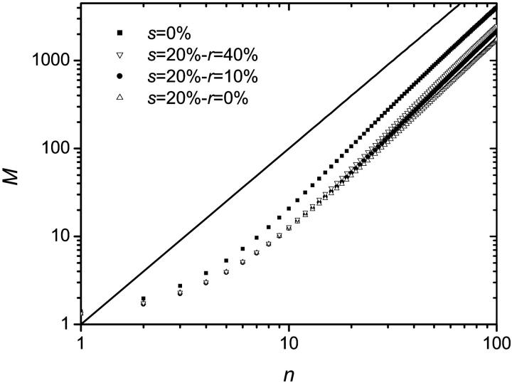
When the probability r that a fertile molecule hybridizes with and completes a sterile molecule is not negligible, the impact of molecular sterility is less important. For example, we can see in Fig. 12 that the s = 0.2 curve gets closer to the s = 0.0 curve as r increases. The effect is very subtle, however, and the recombination mechanism can be neglected if s is not too large. For large values of s, however, rehybridization cannot be neglected because it is the only mechanism that ensures that a colony will not remain surrounded by sterile molecules forever. Rehybridization is then the key to continuous growth.

FIGURE 12.

Average size M of the colonies as a function of the number n of cycles for various values of r. For each set of data the results were averaged over 100,000 colonies and p = 0.4 was used. When the probability r that a fertile molecule hybridizes and completes a sterile molecule is not negligible, the effect of the sterile molecules is a little less important: the s = 0.2 curve gets closer to the s = 0.0 curve as r is increased.

Note that sterile molecules can affect the shape of the colonies. While extremely symmetric when no or only a small fraction of the molecules are sterile, the colonies become more asymmetric when the fraction of the sterile molecules is increased (results not shown). This is so because a small number of consecutive sterile molecules can completely block a direction of growth for the colony. The colony then has to go around the blocked section, leading to an asymmetrical growth.

Detachment

Until now, we have assumed that a primer (or an attached molecule) cannot be removed from the surface. In reality, the successive heating and cooling phases can cause the primer to break away from the surface. The algorithm was further modified to include this rather dramatic effect: at each cycle a molecule now has a probability x of disappearing. It is further assumed that the number of primers remains high and that it is never a limiting factor. Therefore the probability of copying a molecule p is not affected by primer detachment, and remains constant. Furthermore, a site that has just been vacated by the detachment of a molecule cannot be distinguished from a site that has never been occupied. Note that it is also assumed that the detachment of a molecule occurs at the beginning of a thermal cycle in the denaturation phase when the solution is heated and that the probability x is independent of the number of cycles.

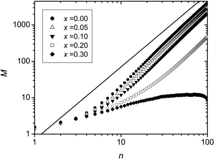
Fig. 13 shows the average size of the colony as a function of the number of cycles for various values of x. The probability for a molecule to make a copy was set to p = 0.4, the sterile molecules were neglected (s = r = 0), the number of thermal cycles was set to n = 100, and the results were averaged over 100,000 colonies. An increase in the probability of molecular detachment results in a decrease of the expected size of the colony. Furthermore, when x reaches a critical value (here x^* ≃ 30%), the expected size of the colony actually decreases after it reaches a maximum. This means that the colonies are actually doomed to becoming extinct as the number of thermal cycles is increased; molecules simply disappear faster than they are created. Note that the data in Fig. 13 are actually an average over the colonies that survive (i.e., colonies that have at least one fertile molecule) at least n = 100 cycles. The argument is that the extinct colonies cannot be observed experimentally. If the extinct colonies are included in the average, the expected size of the colony is further reduced. Another phenomenon associated with the detachment of molecules is that as x increases, there is a possibility that a colony actually splits into two (or more) distinct parts making the results harder to interpret. Note that the actual value of x^* is expected to correspond to the case where the probability of detachment in one cycle is equal to the net duplicating probability for that cycle ((1 − x)p). The value of x^* is thus independent of the lattice type, but depends on the value of p. For p = 0.40, we have 0.4 (1 − x^*) = x^* leading to x^* = 0.2857, which is consistent with our results.

FIGURE 13.

Average size of the colonies M as a function of the number n of cycles for various values of x, the probability for a molecule to break away from the surface. The solid line corresponds to a geometrical growth and has a slope of 2. For each set of data the results were averaged over 100,000 colonies and p = 0.4 was used.

The colony density profile

One drawback to using a lattice to model SPA is that the lattice rigidly fixes the maximum density of molecules (e.g., to one per lattice site). Although a uniform density seems to be a fairly good approximation, one should expect the density at the center of the colony to be somewhat higher than at the fringe. Indeed, while it is very difficult for a molecule surrounded by others to bend so that its end can find a matching primer, it is not completely impossible. This section explores three alternatives to model this phenomenon.

One simple way to model a greater density at the center of the colony is to allow a molecule to make copies of itself on interstitial lattice sites. In practice, the algorithm is modified in the following way: at each cycle, a molecule that is completely surrounded (all its nearest east-west-north-south neighbors are occupied) tries to find a primer in one of the four interstitial sites (chosen randomly) situated in between these neighbors (see Fig. 14). If that site is empty, the molecule has a probability d < p of making a copy.

FIGURE 14.

An example of a lattice with a smaller effective mesh size. At each cycle a main molecule (in black) that is completely surrounded (all its nearest neighbors are occupied) tries to find a primer in one of the four interstitial sites (chosen randomly). If that site is empty, the molecule has a probability d of making a copy (in gray).

Here, the average size of the colonies will be studied as a function of the number of cycles for various values of d assuming p = 0.4, s = r = x = 0, and n = 100. Fig. 15 shows these results, averaged over 100,000 colonies. As expected, the average population size of a colony increases with d. This increase is far from being linear, though. After a fast increase when d is varied from 1% to 5%, a further increase of d causes little change to the average colony size. The reason is that the maximum density is limited, therefore a larger d simply results in a faster increase, but not in a higher density. This is an important finding because it means that the probability that a molecule produces a new copy in a dense environment cannot be neglected even if it is very small.

FIGURE 15.

Average size M of the colony as a function of the number n of cycles for d = 0%, 1%, 5%, 10%, and 20%, where d is the probability that a molecule makes a copy on an interstitial site. For each set of data the results were averaged over 100,000 colonies and p = 0.4 was used. Inset: Same data on a log-log graph. All curves are now almost undistinguishable. The solid line corresponds to a geometrical growth and has a slope of 2.

An alternative way to model a continuous growth at the center of the colony is to let more than one molecule occupy each site in our lattice model. In practice, the algorithm is modified in the following way: at each cycle, a molecule that is completely surrounded tries to duplicate onto its own lattice site. The probability for the duplication to be successful (p_d(N)) depends on the number N of molecules on the site like, e.g.,

(9)

where A is a parameter regulating the strength of the local (on-site) steric interactions. When A → ∞, the system is reduced to the ordinary SPA thermocycled algorithm presented in The Basic System, and colonies grow in a geometrical manner. On the other hand, when A → 0, the system behaves like a perfect solution PCR (with no steric interaction) and the size of the colony grows exponentially. For intermediate values of A, the growth becomes geometric after a transition regime whose duration (number of cycles) depends upon the value of A (a large value of A leads to a short transition period). This transition regime can be observed in Fig. 16, where the average colony size is plotted as a function of the number n of thermal cycles for a value of A = 0.5. The inset of Fig. 16 shows a typical density profile obtained with the algorithm. The density profile of the colony is not flat, unlike the colonies generated in the previous sections.

FIGURE 16.

Average size M of the colony as a function of the number n of thermal cycles for the case where more than one molecule can occupy the same site (see Eq. 9, with A = 0.50). After a fairly long transition time, the colony grows in a geometrical manner. The simulations were performed for up to 200 thermal cycles and were averaged over 200 colonies. Inset: Example of a density profile.

In fact, we can also propose a deterministic analytical model for the growth behavior of such a colony, using a continuous time approximation. In dimensionless units, the model is defined by the differential equation:

(10)

where ρ(r,t) is the local density of the colony at time t, H is the Heaviside (or step) function, v is the radial speed at which the colony grows (one could take this to be roughly given by p since this is the probability for the perimeter to grow out by one more lattice site), and f(ρ) is a function describing the steric influence of the current density on the local growth. Here, r is the distance from the center of the colony (we assume a polar symmetry). Following Eq. 9, we can use, for example, the exponential constraint

(11)

With the blank initial condition ρ(r,0) = 0, we obtain

(12)

The solution can be integrated to obtain the total intensity of the colony as

(13)

The results confirm that the growth is always geometric after a transient regime, and that the density profile of the colony is peaked. Therefore, geometric growth and nonflat profiles are not contradictory. Note that we also tried other f(ρ) functions (e.g., the simple ceiling equation f(ρ) ∼ (ρ_max − ρ)ⁿ), and obtained qualitatively similar results.

DISCUSSION

The simple lattice model of solid phase DNA amplification (SPA) presented in this article predicts major qualitative differences between solution PCR and SPA. First, we find that SPA cannot be characterized by an exponential growth because of the phenomenon of molecular crowding (a chain has less chance to produce an offspring when surrounded by other chains). Therefore, the molecules at the center of the colony slow, or even stop, their duplication and only the perimeter molecules can reproduce freely. The colonies thus grow outwards, i.e., from their perimeter in a geometric manner. An exponential phase can nevertheless be observed in the first few thermal cycles, when the duplication probability of all molecules is little affected by the presence of the others. Another difference between solution PCR and SPA is the probability distribution function for the population of offspring. Because SPA is less sensitive to failures in the first few thermal cycles, the distribution for the population of offspring is much sharper than the one obtained for solution PCR.

SPA characteristics (geometrical growth and sharper size distribution) are unaffected by the addition of sterile molecules or random detachment of molecules if the related probabilities do not reach critical values where they completely stop the growth of the colony. Furthermore, nonflat density profiles, obtain when the molecules at the center of the colony do not completely stop duplicating, still lead to geometrical growth and sharper size distributions than solution PCR.

The present algorithm is based on many educated assumptions currently lacking solid foundations. To test those assumptions and obtain realistic values for the parameters, a combination of precise experimental data and microscopic simulations in which the polymeric nature of the chain is explicitly taken into account, should be used. Among the possible aspects that a microscopic model could address are the time required for the free end to touch the surface and the average spatial distribution of those contacts as a function of the chain density. These simulations would provide some answers to many interrogations. For example, they would give a clear indication on the lattice best suited to model thermocycled SPA and provide a realistic description of the dependence of the probability of making a copy (p) upon the local density. Comparison with experimental data is also undoubtedly required. Growth curves, size distributions, and density profiles should be compared to experimental data to identify the relevant minimal set of parameters and to estimate their numerical values.

A reliable and quantitative model of SPA would help not only to explain experimental data, but also to optimize the experimental procedures. Also, it could be used to model more global phenomena than the growth of single isolated colonies. For example it could easily be used to model the interaction between two (or more) colonies with different characteristics.

References

- Adessi, C., G. Matton, G. Ayala, G. Turcatti, J.-J. Mermod, P. Mayer, and E. Kawashima. 2000. Solid phase amplification: characterisation of primer attachment and amplification mechanisms. Nucleic Acids Res. 28:e87. [DOI] [PMC free article] [PubMed] [Google Scholar]
- Bailey, N. T. J. 1963. The Element of Stochastic Processes. Wiley Classics Library, Oxford, UK.
- Bing, D. H., C. Boles, F. N. Rehman, M. Audeh, M. Belmarsh, B. Kelley, and C. P. Adams. 1996. Bridge amplification: a solid phase PCR system for the amplification and detection of allelic differences in single copy genes. In Genetic Identity Conference Proceedings, Seventh International Symposium on Human Identification, http://www.promega.com/geneticidproc/ussymp7proc/0726.html.
- Boom, R., C. Sol, Y. Gerrits, M. D. Boer, and P. W. van Dillen. 2002. Highly sensitive assay for detection and quantitation of human cytomegalovirus DNA in serum and plasma by PCR and electrochemiluminescence. J. Clin. Microbiol. 37:1489–1497. [DOI] [PMC free article] [PubMed] [Google Scholar]
- Brownie, J., S. Shawcross, J. Theaker, D. Whitcombe, R. Ferrie, C. Newton, and S. Little. 1997. The elimination of primer-dimer accumulation in PCR. Nucleic Acids Res. 25:3235–3241. [DOI] [PMC free article] [PubMed] [Google Scholar]
- Currie, E. P. K., G. J. Fleer, M. A. C. Stuart, and O. V. Borisov. 2000. Grafted polymers with annealed excluded volume: a model for surfactant association in brushes. Eur. Phys. J. E. 1:27–40. [Google Scholar]
- Eden, M. 1961. A two-dimensional growth process. In Proceedings of the 4th Berkeley Symposium on Mathematical Statistics and Probability. University of California Press, Berkeley, CA. pp.223–239.
- Feller, W. 1968. An Introduction to Probability Theory and its Applications, vol. 1. John Wiley and Sons, New York.
- Halford, W. P., V. C. Falco, B. M. Gebhardt, and D. J. J. Carr. 1999. The inherent quantitative capacity of the reverse transcription polymerase chain reaction. Anal. Biochem. 266:181–191. [DOI] [PubMed] [Google Scholar]
- He, Q. A., J. Wang, M. Osato, and L. B. Lachman. 2002. Real-time quantitative PCR for detection of Helicobacter pylori. J. Clin. Microbiol. 40:3720–3728. [DOI] [PMC free article] [PubMed] [Google Scholar]
- Hogdall, E., K. Boye, and J. Vuust. 1999. Simple preparation method of PCR fragments for automated DNA sequencing. J. Cell. Biochem. 73:433–436. [PubMed] [Google Scholar]
- Markoulatos, P., N. Siafakas, and M. Moncany. 2002. Multiplex polymerase chain reaction: a practical approach. J. Clin. Lab. Anal. 16:47–51. [DOI] [PMC free article] [PubMed] [Google Scholar]
- Meinhardt, H. 1982. Models of Biological Pattern Formation. Academic Press, London.
- Nazarenko, I., B. A. Lowe, M. Darfler, P. Ikonomi, D. Schuster, and A. Rashtchian. 2002. Multiplex quantitative PCR using self-quenched primers labeled with a single fluorophore. Nucleic Acids Res. 30:e37. [DOI] [PMC free article] [PubMed] [Google Scholar]
- Netz, R. R., and M. Schick. 1998. Polymer brushes: from self-consistent field theory to classical theory. Macromolecules. 31:5105–5140. [DOI] [PubMed] [Google Scholar]
- Pang, Y. S., H. Wang, T. Girshick, Z. X. Xie, and M. I. Khan. 2002. Development and application of a multiplex polymerase chain reaction for avian respiratory agents. Avian Dis. 43:691–699. [DOI] [PubMed] [Google Scholar]
- Peccoud, J., and C. Jacob. 1996. Theoretical uncertainty of measurements using quantitative polymerase chain reaction. Biophys. J. 71:101–118. [DOI] [PMC free article] [PubMed] [Google Scholar]
- Sams, T., K. Sneppen, M. H. Jensen, C. Ellegaard, B. E. Christensen, and U. Thrane. 1997. Morphological instabilities in a growing yeast colony: experiment and theory. Phys. Rev. Lett. 79:313–316. [Google Scholar]
- Skvortsov, A. M., A. A. Gorbunov, and F. A. M. L. G. J. Fleer. 1999. Long minority chains in a polymer brush: a first-order adsorption transition. Macromolecules. 32:2004–2015. [Google Scholar]
- Stauffrer, D., and A. Aharony. 1992. Introduction to Percolation Theory. Taylor and Francis, London, UK.
- Stevens, S. J. C., I. Pronk, and J. M. Middeldorp. 2002. Toward standardization of Epstein-Barr virus DNA load monitoring: unfractionated whole blood as preferred clinical specimen. J. Clin. Microbiol. 39:1211–1216. [DOI] [PMC free article] [PubMed] [Google Scholar]
- Wabuyele, M. B., and S. A. Soper. 2001. PCR amplification and sequencing of single copy DNA molecules. Single Mol. 2:13–21. [Google Scholar]
- Wagner, G., R. Halvorsrud, and P. Meakin. 1999. Extended Eden model reproduces growth of an acellular slime mold. Phys. Rev. E. 60:5879–5887. [DOI] [PubMed] [Google Scholar]
- Williams, T., and R. Bjerknes. 1972. Stochastic model for abnormal clone spread through epithelial basal layer. Nature. 236:19–21. [DOI] [PubMed] [Google Scholar]
- Ziqin, W., and L. Boquan. 1995. Random successive growth model for pattern formation. Phys. Rev. E. 51:R16–R19. [DOI] [PubMed] [Google Scholar]