Kinetics of Prion Growth

Abstract

We study the kinetics of prion fibril growth, described by the nucleated polymerization model analytically and by means of numerical experiments. The elementary processes of prion fibril formation lead us to a set of differential equations for the number of fibrils, their total mass, and the number of prion monomers. In difference to previous studies we analyze this set by explicitly taking into account the time-dependence of the prion monomer concentration. The theoretical results agree with experimental data, whereas the generally accepted hypothesis of constant monomer concentration leads to a fibril growth behavior which is not in agreement with experiments. The obtained size distribution of the prion fibril aggregates is shifted significantly toward shorter lengths as compared to earlier results, which leads to a enhanced infectivity of the prion material. Finally, we study the effect of filtering of the inoculated material on the incubation time of the disease.

INTRODUCTION

Although the detailed mechanism for the spreading of transmittable spongiform encephalopathies diseases (TSE) such as scrapie, kuru, and a kind of Creutzfeld-Jacob disease is not yet convincingly clarified, by now it is generally acknowledged that prion proteins are involved in all forms of TSE diseases (e.g., Laplanche et al., 1999; Will et al., 1999; Parchi et al., 1996). There is a long history of speculations, starting as early as 1967 (Alper et al., 1967; Griffith, 1967), on whether the presence of misfolded and fibril-like structure-forming prions cause the disease or whether they are just a side effect accompanying the disease. By now, however, there is still no rigorous experimental proof of any of these hypotheses.

The prion involved in TSE diseases is the PrP protein (Prusiner, 1991). It is found in two distinct conformations, PrP^c and PrP^sc. The proteins of PrP^c (c for cellular) conformation are located at the surface of neural tissues, but their function has not yet been revealed. In difference to the healthy conformation, PrP^c, the pathogenetic conformation of this protein, called PrP^sc (sc for scrapie), is only partially digested by proteinase K. The most striking feature of PrP^sc is that it tends to form large-scale aggregates (Jeffrey et al., 1995) comprising ∼200 monomeric units (Prusiner, 1999a). These fibrillic aggregates are essentially one-dimensional structures (Jarrett and Lansbury, 1993; Lansbury and Caughey, 1995), whose sizes grow along one dimension in both linear directions (Scheibel et al., 2001).

For the molecular mechanism of the conversion of the healthy PrP^c molecule into the pathological PrP^sc several models have been proposed, such as the hetero-dimer mechanism (Cohen et al., 1994), the cooperative autocatalysis (Eigen, 1996), and the nucleated polymerization model (Jarrett and Lansbury, 1993). In a critical comparison of these models, Masel and co-workers gave arguments in favor of the nucleated polymerization model (Masel et al., 1999), which by now seems to be widely accepted. Since the kinetic theory which will be presented in the following sections applies to this model, we wish to briefly sketch it here: it is assumed that, in the PrP^c conformation, prions occur as monomers, whereas aggregates consist of PrP^sc. The process of polymerization is assumed to be extremely slow until a threshold size of n monomers in the aggregate is achieved. Above this critical size the polymer is much more stable, and the polymerization progresses significantly faster (Lansbury and Caughey, 1995). PrP^sc polymers are assumed to be unbranched, i.e., they are effectively one-dimensional. It does not necessarily mean, however, that the PrP^sc macromolecules are one-monomer wide; i.e., they may well have helical or similar structure.

Hence, the model by Masel et al. (1999) addresses the evolution of the disease after an external infection. It does not describe the aggregate formation by polymerization of monomers, i.e., the appearance of sporadic prion diseases. The evolution of the disease after an infection can be described separately since the polymerization of monomers (to form stable aggregate of supercritical size) is a very slow process. Aggregates which contain a number of monomers less than n are energetically unfavorable, inasmuch as they cannot form a stable fold such as a complete β-helix (Wille et al., 2002). Therefore it is assumed that, once created, subcritical aggregates disintegrate almost immediately into monomers.

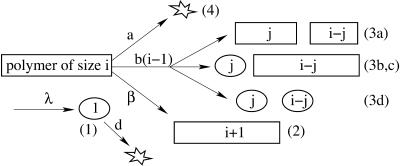
Thus, the following elementary processes are involved in the kinetic model by Masel et al. (1999):

1. The system contains a variable number x of PrP^c monomers. They are generated at a time-independent rate λ. Each PrP^c monomer is degraded metabolically at rate d. Thus, by generation, one obtains x → x + 1, by degradation x → x − 1.

2. Each of the linear PrP^sc polymers grows by one monomer unit with rate β. If we denote the number of PrP^sc molecules of length i by y_i, then growth of a polymer of length i by incorporating a monomer causes y_i → y_i − 1, y_i+1 → y_i+1 + 1, and x → x − 1.

3. Any PrP^sc polymer of size i may split into two smaller polymers. Inasmuch as a linear polymer of length i has i − 1 links connecting monomeric units and each of them may break at rate b, a PrP^sc polymer splits at rate b(i − 1) into two smaller pieces of lengths j ∈ [1, i − 1] and i − j. If the length of one or both of the fragment polymers is smaller than the minimal stable polymer size n, this fragment(s) disintegrates into PrP^c monomers. The latter process is assumed to occur very rapidly, i.e., an infinite rate is assumed.

   Hence, the split of a polymer of size i into two smaller pieces of sizes j and i − j causes the following changes of the system's status:

   • (a) if j ≥ n and i − j ≥ n: , , , or
   • (b) if j < n and i − j ≥ n: , , , or
   • (c) if j ≥ n and i − j < n: , , , or
   • (d) if j < n and i − j < n: , .

   Note that the last rule, (d), deviates from the model proposed by Masel et al. (1999). In their model, the case j < n and i − j < n was not explicitly considered. If a polymer of size smaller than 2n − 2 splits it may happen that both of the arising smaller polymers are shorter than the minimum stable length n. If one does not take into account rule (d), only one of them disintegrates into monomers—which is inconsistent with the assumption that polymers shorter than n are unstable. By means of rule (d), we assure that both polymers disintegrate, provided both of them are smaller than n.

4. A PrP^sc polymer may be degraded by incorporation into plaques or by engulfment by macrophages. This process is independent of the size of the polymer and occurs at rate a. Here the transition y_i → y_i − 1 occurs.

The described prion growth model is sketched in Fig. 1 .

FIGURE 1.

Sketch of the prion aggregate growth model after Masel et al. (1999) but modified. For explanation see text.

The aim of this article is to outline some consequences which follow from the mathematical analysis of the nucleated polymerization model of PrP^sc molecule growth. In particular we show that there exists a stable steady-state normalized size distribution of PrP^sc polymers for which we provide an explicit analytical expression. We describe quantitatively the dynamics of the average size of PrP^sc polymers and give evidence for qualitatively different scenarios of the disease which happen after an inoculation of PrP^sc into a healthy organism. We derive a condition which discriminates the scenario of healing, when the initial number of PrP^sc molecules due to the inoculation decays to zero, from different scenarios. In difference to earlier results we give evidence that asymptotically the exponential growth of the total PrP^sc mass ceases and the system finally relaxes to a steady state with a well-defined size distribution of polymers. In this steady state the numbers y_k of polymers of lengths k is constant, as well as the number of monomers. The steady state of the system is determined by the rate constants a, b, and β, but not by λ and d, which characterize the monomer production and degradation, even if both of these rates are large as compared to other rates in the system.

We wish to note that although the nucleated polymerization model by Masel et al. (1999) is widely accepted, there exist also alternative models of the prion-related diseases. Wille et al. (2002) claimed that the formation of aggregates is not the main process in such diseases and that nonfibrillar structures of the PrP^sc may be important. The authors emphasized that the conversion of PrP^c into PrP^sc is driven by the formation of unusually stable parallel β-helix folds. Serio et al. (2000) proposed a conformational conversion model, which incorporates both the aspects of the nucleated polymerization and templated assembly models (Prusiner, 1999b) with some additional features. The authors suggest that the appearance of the fibrillar structures during prion-related diseases happens due to the aggregation of oligomeric intermediates.

DERIVATION OF THE KINETIC EQUATIONS

Consider the rate equations for all species involved in the dynamics of PrP^sc growth. The numbers in curled brackets, {…}, refer to the enumeration of the elementary processes as described in the previous section. We denote the time-dependent number of PrP^c monomers by x(t), and of PrP^sc polymers by y_k(t) with k being the degree of polymerization, i.e., the length of the polymer.

In what follows we do not consider spatial effects for the reaction kinetics, i.e., we assume that the above-mentioned elementary processes occur independently of the spatial location of the polymers and monomers. A complete model should account for such spatial effects and describe the transport of monomers and polymers of different sizes in the organism. Spatial effects may affect the reaction rates considerably. Moreover such effects as the spread of the infection from the place of injection to the place of observation (which may cause a time lag in the evolution of the disease) need to be considered by a model which takes into account spatial effects. Presently, however, we do not have a reliable model of the molecular transport in the organism and thus we restrict ourselves to the here-presented simplified model.

The PrP^c monomer equation

According to the model by Masel et al. (1999) there are two different source terms for x(t), namely the generation of PrP^c monomers with rate λ {1} and disintegration of split products of length smaller than n {3b,3c,3d}. Sink terms for PrP^c monomers are caused by metabolic degradation at rate d {1} and by PrP^sc polymer growth {2}. Mathematically, the rate equation for PrP^c monomers that takes into account these four processes reads

(1)

The meaning of the first two terms at the right-hand side of Eq. 1 is obvious. The third term describes aggregation of monomers with polymers of different sizes, where one has to take into account all existing degrees of polymerization, starting from i = n, since polymers of size smaller than n are unstable.

The instability of polymers smaller than n is explicitly accounted by the following two terms: the index j refers to the size of one piece after the fracture of a polymer of size i (which occurs in y_i copies). For , this piece disintegrates and produces j monomers. Since the piece of size j may be split from both sides of the polymer, the breakage rate constant b doubles in Eq. 1. It is assumed that a polymer of length i can split at i − 1 positions and all of these splittings occur with equal rate b. This term describes the process when only one of the fragments is smaller than n, whereas the other one of size i − j ≥ n is stable. The last term in Eq. 1 accounts for the process when both products of the splitting process are smaller than n. In this case both of the resulting polymers are completely disintegrated and, thus, produce i monomers. Note that in the mathematical formulation of the model given by Masel et al. (1999) the possibility of complete disintegration of the polymer after splitting was not taken into account and the equation for the monomers derived there lacks the corresponding term. At first glance, this term that concerns only polymers of lengths smaller than 2n − 2, should not essentially affect the distribution y_i(t). The term matters, however, since splitting such a small molecule due to the original rule would produce a number of PrP^c monomers and a PrP^sc polymer of length smaller than n which is assumed to be unstable by definition. Hence, neglecting this term any simulation would produce polymers of size smaller than n and, hence, lead the system into an ill-defined state.

The PrP^sc polymer equation

Next we write the rate equations for the PrP^sc polymers. The elementary processes as described at the end of the Introduction give rise to the kinetic equations for the number of PrP^sc polymers of length i ≥ n,

(2)

The first term at the right-hand side of Eq. 2 describes the growths of the number of PrP^sc polymers of size i when a monomer reacts with a PrP^sc polymer of size i − 1 (process {2}), transforming it into a polymer of size i. Similarly, the second term describes the reaction of a polymer of size i with a monomer which transforms it into a polymer of size i + 1 by reducing the number y_i. The third term describes the degradation of PrP^sc polymers independent of their size (process {4}), with the rate . The fourth term refers to all possible splittings of the polymer of size i, which leads to decreasing y_i. Indeed, the total rate of all possible splittings of polymer i into pieces of l and i – l with equal rate b reads

(3)

Finally, the last term describes the process when a polymer of size j splits into two pieces—one of length i, and the other one which may be of any size. Again, the rate constant b doubles, since the piece i may be split from both ends of the polymer.

Important characteristics of the size-polydisperse PrP^sc polymer solution are the total number of polymers y and the total number of monomers which are contained in the abundance of these polymers z as

(4)

where z is proportional to the total mass of PrP^sc.

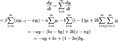
An equation for y may be obtained by summing up all Eqs. 2 for all polymer sizes i:

(5)

To simplify Eq. 5, we use the definitions from Eq. 4 and the identity of

(6)

which holds true, inasmuch as y_n−1 = 0. The last term in Eq. 5 simplifies as

(7)

where the step-function is defined by

(8)

With Eqs. 6–7 we arrive at

(9)

Similarly, multiplying the i^th equation in Eq. 2 by i and performing the summation we obtain an equation for z(t) of

(10)

Although the equation for the number of monomers was incomplete in Masel et al. (1999), Eqs. 9 and 10 coincide with those obtained there. This does not mean that the time dependence of the number of polymers y(t) and their total mass z(t) is identical to previous results, since the number of monomers, x(t), enters the equations for y and z. We will show below that the evolution of y(t) and z(t) is even qualitatively different from that of the model by Masel et al. (1999).

Collecting the results of this section, we give the set of equations that govern the evolution of the system:

(11)

Unfortunately, with the correct kinetic equation for the monomers it is not possible to obtain a closed solution for the variables x, y, and z. In general, the evolution of monomers x depends not only on the total number of polymers y and their total mass z, but on the full distribution y_k, which is unknown. We will come back to this issue in The Effect of Filtering.

KINETIC EQUATIONS FOR CONSTANT NUMBER OF MONOMERS

Simplified set of equations for x(t) = x₀ = const

The analysis of the kinetic equations in Eq. 11 simplifies considerably if one assumes that the number of PrP^c monomers is kept constant by some regulatory processes in the cell:

(12)

With this assumption, the rates in Eq. 11 simplify to a set of linear equations:

(13)

which may be solved exactly. The solution reads (Masel and Jansen, 2001),

(14)

(15)

with

(16)

In realistic systems we have r₁ > 0, r₂ < 0 (Masel and Jansen, 2001). The constants c₁, c₂, d₁, and d₂ are specified by the initial conditions, i.e., they may be expressed in terms of y(0) and z(0):

(17)

Hence, the time-dependence of y(t) and z(t) is described by two exponents, r₁ and r₂.

PrP^sc polymer size distribution

The equations for the number of polymers with different degree of polymerization may be found iteratively. The evolution of y_n(t) is characterized by three exponents, y_n+1 by four exponents, and generally, y_n+k(t) by k + 3 exponents. To show this, we apply the Laplace transformation

(18)

to the kinetic Eq. 2 for the number of polymers. We use the property of the Laplace transform and write as . Then the Laplace transform of y_k reads

(19)

Inasmuch as the Laplace transform of y(t) and z(t) is given by

(20)

may be expressed by means of Eq. 19 in terms of with j < k. Hence, Eq. 19 allows for an iterative solution for the complete polymer size distribution, starting from (y_j = 0 for j < n). It reads

(21)

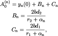
where we introduce the short-hand notation, α_k ≡ βx₀ + a + b(k + 1). The inverse Laplace transform for these simple fractions (which correspond to the basic inverse Laplace transforms; Abramowitz and Stegun, 1964) reads as

(22)

with

(23)

where we take into account that r₂ < 0. As it follows from Eq. 22, the evolution of y_n is described by three exponential functions. Similarly, may be expressed in terms of and . Performing the inverse Laplace transform for this quantity yields

(24)

where the coefficient depends on y_n(0), on y_n(0) and , whereas the coefficients and depend only on y(0) and z(0). The expressions for these coefficients are derived in Appendix B.

Thus, y_n+1(t) is expressed by four exponents. This iterative procedure may be continued to find successively all y_k(t), i.e., the complete polymer size distribution. Using Eqs. 22 and 24 and the iterative scheme, one obtains the time-dependence of the polymer size distribution,

(25)

where , B_i, and C_i are constants and the coefficients α_j have been defined above. As already mentioned, for realistic parameters r₁ > 0 and r₂ < 0, thus in the series of expressions in Eq. 25 only the last term has a positive exponent and grows with time. Therefore, after a transient time which is considerably shorter than the incubation time (Masel and Jansen, 2001), all terms with negative exponents may be neglected. This means that the system evolves independently of its initial conditions and the distribution of PrP^sc polymer sizes has achieved its steady-state form. Neglecting the amplitudes and B_i, one obtains expressions for the coefficients C_i. Solving this equation (details are given in Appendix B), one obtains the steady-state distribution for the normalized size distribution w_i = y_i/y:

(26)

where

(27)

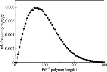
Fig. 2 shows the analytical result, Eq. 26, together with the results of a numerical simulation. The details of the simulation method are given in Appendix A.

FIGURE 2.

Distribution of polymers w_i ≡ y_i/y over the polymer length i for fixed number of monomers x₀ = 500. We obtain excellent agreement between the analytical result Eq. 26 (line) and the results of a numerical simulation (circles). The parameters are n = 6, a = 0.05, b = 9 × 10⁻⁴, and β = 0.015.

Evolution of the average size of PrP^sc polymers and scenarios of PrP^sc evolution

We introduce the average size of PrP^sc polymers as s(t) = z(t)/y(t). Both y(t) and z(t) have the same time-dependence after the transient time, which corresponds to exponential growth with the exponent r₁ as given in Eq. 16. Therefore, the average size is time-independent after this transient time. From the set of equations in Eq. 13 for y(t) and z(t) follows the equation for s:

(28)

(29)

Equation 29 defines the value of γ = βx₀ − bn(n − 1).

The solution of Eq. 28 reads

(30)

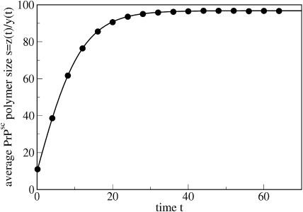
with s(0) being the initial average length of PrP^sc polymers. The evolution of the average size as described by Eq. 30 is drawn in Fig. 3 together with the results of a numerical simulation of the stochastic model. Solving the steady-state equation

(31)

we obtain for the steady-state average size

(32)

The number of PrP^sc molecules y(t) can also be expressed in terms of the average polymer size s(t). From Eq. 13 follows

(33)

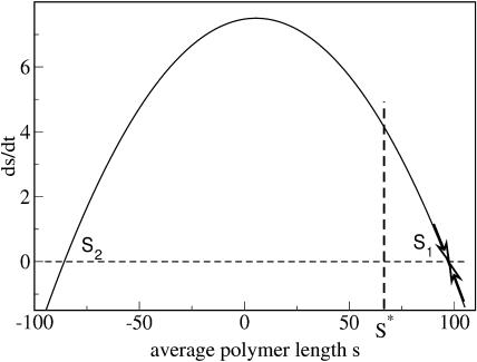
The velocity of growth of the average size as a function of the average size s is drawn in Fig. 4. For the given set of parameters the values of s_1/2 and s^* are marked. We see that only the steady-state solution s₁ corresponds to a stable fixpoint (moreover, for the chosen set of parameters, s₂ is negative).

FIGURE 3.

Evolution of the average size s = z(t)/y(t) of PrP^sc polymers due to Eq. 30 (line) and results of a simulation (circles). The parameters are n = 6, a = 0.05, b = 9 × 10⁻⁴, and β = 0.015. The initial size is s(0) = 10.

FIGURE 4.

The average growth velocity over the average size s due to Eq. 29. The parameters are n = 6, a = 0.015, b = 0.0009, β = 0.025, and x₀ = 500.

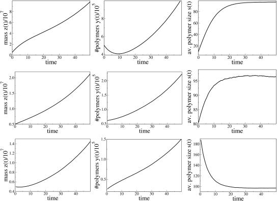
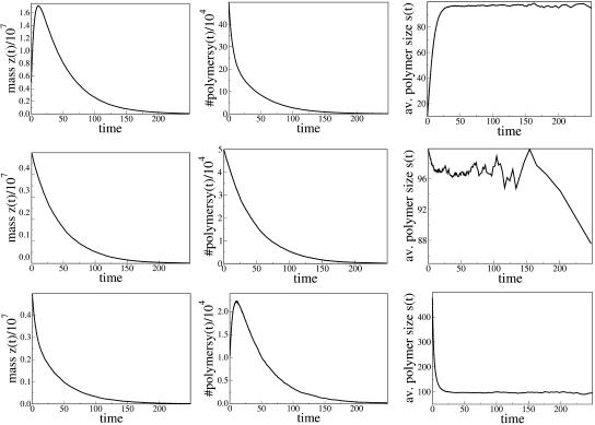
From Eq. 33 one can conclude that there exist several scenarios of the system evolution, depending on the initial mean size of polymers s(0) (see Figs. 5 and 6).

FIGURE 5.

PrP^sc polymer growth scenarios for the case s^* < s₁. The parameters are n = 6, a = 0.05, b = 9 × 10⁻⁴, and β = 0.015, which corresponds to s^* = 66.44 and s₁ = 96.78. (Top) s(0) < s^* (y₁₀(0) = 5 × 10⁵); (middle) s(0) > s^* (y₂₅(0) = 8 × 10³); and (bottom) s(0) > s₁ (y₂₀₀(0) = 25,000). In all cases the initial inoculation is z(0) = 5 × 10⁶.

FIGURE 6.

PrP^sc polymer growth scenarios for the case s^* > s₁. The parameters are the same as in Fig. 5 except for a = 0.1, which corresponds to s^* = 122.11 and s₁ = 96.76. (Top) s(0) < s₁ (y₁₀(0) = 5 × 10⁵); (middle) s^* > s(0) > s₁ (y₁₀₀(0) = 5 × 10⁴); and (bottom) s(0) > s^* (y₅₀₀(0) = 10⁴). In all cases the total initial inoculation is z(0) = 5 × 10⁶.

The last three cases (Fig. 6) correspond to decay of the total number of polymers to zero. Any inoculation for the corresponding sets of parameters does not lead to spreading of the disease. The condition of complete recovery of an infected organism reads s₁ < s^*, or in terms of the number of monomers,

(34)

where

(35)

Contrarily, if the condition of Eq. 34 does not hold, any inoculation of PrP^sc polymers leads to infection, even if the inoculation is infinitesimally small, e.g., consists of a single molecule. Certainly this is not realistic and demonstrates that the application of continuum differential equations has a restriction. These deal with the average numbers and ignore their fluctuations. For very dilute systems the fluctuations of the numbers of molecules are of the same order as the numbers themselves and one has to use a stochastic model, which is employed in the present study (see Appendix A).

THE FULL SET OF KINETIC EQUATIONS, EQ. 11

Evolution of x(t), y(t), and z(t)

So far the number of PrP^c monomers was kept constant (x(t) = x₀), which was attributed to some regulatory process. This assumption simplifies the analysis of the kinetic equations yielding the linear set of Eq. 13, which enables us to draw certain conclusions as shown in the previous sections.

Unfortunately, we are not able to solve the full set of equations in Eq. 11 including the time-dependence of PrP^c monomers in a closed form. Nevertheless, it is possible to investigate the process sketched in Fig. 1 numerically using a stochastic method, such as the Gillespie algorithm (Gillespie, 1976; Feistel, 1976, 1977; see also Appendix A, this article).

Numerical simulations show that after the initial exponential growth of the number of polymers and of their total mass, the supply of monomers (which occurs at the constant rate λ) is not large enough to support further exponential growth. The system relaxes to the steady state at which the process of PrP^sc decay is completely compensated by the process of their production from PrP^c monomers. After the exponential growth ceases, the number of monomers as well as the number of polymers reach relatively fast their steady-state value x(t) = x_st and The same happens to the total number of PrP^sc polymers y(t) and to their total mass z(t), which also achieve their steady-state values, y_st and z_st.

The expressions in Eq. 11 read for the steady-state case, when and x = x_st, y = y_st, z = z_st,

(36)

From the first equation in Eq. 36 we find the steady-state value of the average size of PrP^sc polymers,

(37)

which, substituted into the second equation in Eq. 36, yields the steady-state number of monomers,

(38)

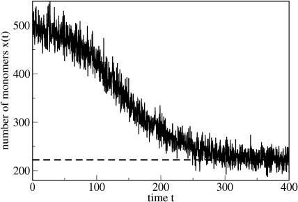
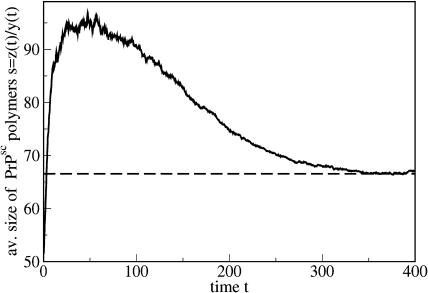
The evolution of the number of monomers and of the average size of polymers is drawn in Figs. 7 and 8.

FIGURE 7.

Evolution of the number of monomers x = x(t). The simulation starts with x(0) = 100 monomers and relaxes within a very short time (which is not visible on the timescale of the figure) to x(t) ≈ 500. This corresponds to the number of monomers x₀ = λ/d which provides the initial exponential growth. According to a complicated dynamics it eventually approaches its steady-state value x_st = 222.211 given by Eq. 38 (dashed line). The parameters are n = 6, a = 0.05, b = 9 × 10⁻⁴, β = 0.015, λ = 200,000, and d = 400.

FIGURE 8.

Evolution of the average size of PrP^sc polymers s = z(t)/y(t). The simulation starts with s(0) = 200. The dashed line shows the analytical result, Eq. 37. The parameters are given in the caption of Fig. 7.

Note that x_st equals the threshold value for the number of monomer x^* for the model with fixed x = x₀. This is not surprising, inasmuch as x^* separates two regimes of exponential decay and exponential growth of the abundance of PrP^sc; thus, x = x_st = x^* corresponds to the number of monomers which keeps the abundance of PrP^sc constant.

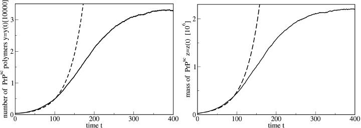
Due to the time-dependence of the number of monomers x(t), the evolution of the number of PrP^sc polymers y(t) and their total mass z(t) becomes more complicated (see Fig. 9): The initial exponential growth finally completely ceases and y(t) and z(t) saturate at their steady-state values. Between the exponential growth and saturation one observes a nearly linear growth.

FIGURE 9.

Evolution of the number of PrP^sc polymers y(t) (left) and the total mass of polymers z(t). For comparison, the dashed lines show the solution of the simplified set of equations, Eq. 14, with the exponents and coefficients given by Eqs. 16 and 17, respectively, with x₀ = λ/d. The parameters of the simulation are given in the caption of Fig. 7.

Steady-state PrP^sc polymer size distribution

The steady-state distribution of the PrP^sc polymer sizes may be obtained exactly in the same way as for the case of x(t) = x₀. The only difference is that instead of x₀ one has to use now x_st, given by Eq. 38, and that the growth rate is zero, i.e., the value of r₁ = 0 is to be taken. Performing the same derivation as presented in Appendix B, but with r₁ = 0, we obtain the steady-state size distribution w_i = y_i/y of PrP^sc polymers:

(39)

with the modified coefficients

(40)

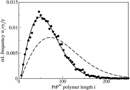
As it follows from Eq. 39, the steady-state distribution is shifted now to smaller polymer sizes as compared to the previous case of x = x₀ (see Eq. 26), where we assumed that the number of PrP^c monomers was kept constant due to some external regulatory process. The size distribution due to Eq. 39 is drawn in Fig. 10.

FIGURE 10.

Size distributions of PrP^sc polymers for the full model, including x = x(t). The points display numerical simulations and the line shows the analytical result, Eq. 39. The parameters of the simulation are given in the caption of Fig. 7. For comparison, the dashed line shows the result for the simplified model with x(t) = λ/d = const. due to Eq. 26.

In Fig. 7 we have drawn the evolution of the number of PrP^c monomers x(t). The rates which are related to the stochastic growth, degradation, and splitting of the PrP^sc polymers are much smaller than the rates of production and degradation of PrP^c monomers, λ and d, respectively (see Masel et al., 1999). This fact gave rise to the assumption of a time-independent number of monomers x(t) = x₀ =λ/d which was exploited in the previous sections. Indeed, shortly after the beginning of the simulation, x(t) relaxes to its assumed steady-state value x₀. For later times, however, one observes a further relaxation to a final steady state.

Evolution of the PrP^sc size distribution

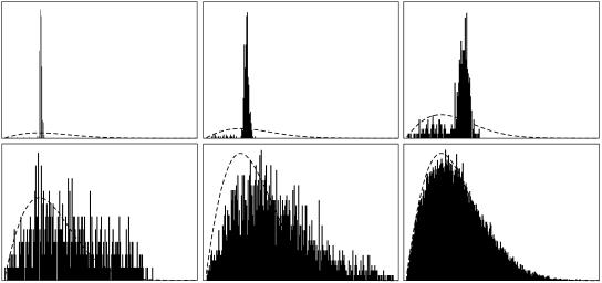
In the previous subsection, we have investigated the steady state of the PrP^sc polymer size distribution. For the spreading of the sickness it may be interesting to know the evolution of the size distribution after an inoculation. In Fig. 11 we have drawn the size distribution at particular times after an inoculation of 435 PrP^sc polymers of length 50 each, i.e., y₅₀(0) = 435. Hence, the total initial PrP^sc mass is z(0) = 435 × 50 = 21750, which is ∼1/100 of the steady-state value as can be seen from Fig. 9 (right). The curves are drawn at time instants t ≈ 0, t ≈ 4, t ≈ 16, t ≈ 64, t ≈ 256, and t ≈ 1024.

FIGURE 11.

Evolution of the size distribution for the initial condition y₅₀(0) = 435, y_i(0) = 0 for i ≠ 50. The parameters of the simulation are given in the caption of Fig. 7.

During the relaxation the distribution shifts significantly to the right, i.e., larger polymers occur preferably. This explains the maximum in the evolution of the average size as drawn in Fig. 8.

The effect of filtering

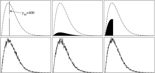
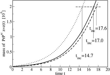
One may raise the question of how the initial PrP^sc length distribution affects the spreading of the disease. To this end we made simulations with identical masses of the initial inoculation, z(0) = 16,000, but with different size distributions. We have chosen three initial distributions, displayed in the top row of Fig. 12. For the simplest one we use a delta-like distribution, y₄₀(0) = 400 (left). As the system evolves it approaches the steady-state distribution as given above (Fig. 10). In Fig. 12 (bottom left) we show the size distribution at the time instant t = 16.1 days when the total mass reaches z = 2 × 10⁶. For the reasons explained below we use this total mass as the mass accumulated after the incubation time, i.e., z(t_inc) = z_inc = 2 × 10⁶. Then this distribution y_i(t_inc) was used to generate two other distributions: the “natural” distribution, y_i(0) = y_i(t_inc)/125 (top middle in Fig. 12) and the “filtered” distribution, y_i(0) = 0 for i > 50 (top right in Fig. 12), preserving the total initial mass z(0). The dashed lines show the (accordingly scaled) distribution y_i(t_inc) which refers to the assumed incubation time. The second row in Fig. 12 shows the according distributions at the incubation time t = 16.1. One notes that at this stage, the initial distribution is already completely relaxed, i.e., there is no significant difference between all the three distributions. The initial distribution does, however, affect the growth of the total mass of PrP^sc molecules. Fig. 13 shows the total mass of polymers over time corresponding to the three different initializations.

FIGURE 12.

Influence of the size distribution of the inoculation to the evolution of the distribution. The parameters are n = 6, d = 100, a = 0.027, b = 0.0048, λ = 10⁶, and β = 0.025. For explanation, see text.

FIGURE 13.

Total mass of PrP^sc molecules, z(t) over time for different initial size distributions as shown in Fig. 12. The initial total mass, z(0) = 16,000, is identical in all cases. The full line corresponds to the left plot in Fig. 12, the dashed line to the middle plot, and the dotted line to the filtered inoculation drawn in the right plot.

It was shown that infected mice develop symptoms of the sickness as soon as there is a certain level of PrP^sc in their brain, independently of the incubation period and the amount of initial inoculation (Manson et al., 1994; Büeler et al., 1994). Therefore, one may define the incubation time t_inc as the time when a certain mass of PrP^sc molecules, z(t_inc) = z_inc, is achieved after an initial inoculation at time t = 0. In Fig. 13 we have marked the times t_inc after which the mass z_inc = 2 × 10⁶ was reached for our three different initial distributions. As it has been already mentioned the initial stage of the disease corresponds to exponential growth of the prion abundance. For the chosen set of the model parameters in Fig. 13, the exponential growth corresponds to the doubling time of ∼2.5 days. This is consistent with the experimental data by Beekes et al. (1996), Taylor et al. (2000), Kimberlin and Walker (1977, 1980, 1986), and Kimberlin et al. (1983), where doubling time in the range of 2–7 days has been reported. Naturally, the exponential growth of the aggregate mass implies linear dependence of the incubation time on the logarithm of the initial dose (Masel et al., 1999). Note, however, that in Fig. 13 the initial dose z(0) is the same for all shown curves; the inoculation differs only by the initial size distribution of the polymers. To illustrate qualitatively the incubation time-dependence on the initial distribution we have chosen z_inc = 2 × 10⁶, which approximately corresponds to 2 LD₅₀ doses (Beekes et al., 1996) and to t_inc = 16.1 days. The ratio z_inc/z(0) ∼1/125 and the incubation time are significantly smaller than those detected in experiments. The experimental incubation time may be 10× larger, whereas the ratio z_inc/z(0) may be as large as 10¹² for low initial doses (see, e.g., Beekes et al., 1996; Taylor et al., 2000). In our simulation, the ratio z_inc/z(0) corresponds to seven doublings—whereas in experiments, ∼20–30 doublings are observed. This ratio, however, is far beyond the abilities of the present computer model based on the Gillespie algorithm. Hence for the qualitative analysis we use the above values for t_inc and z_inc, which can be called “model” values.

Since the initial size distribution affects the growth of the total PrP^sc mass, one may ask the question of how filtering the inoculated material affects the evolution of the total mass and, hence, the incubation time. By filtering at a level k (which is to eliminate PrP^sc polymers whose length exceeds k) from the distribution y_i(t_inc), corresponding to the incubation time, and by preserving the total mass of the inoculated material, i.e.,

(41)

where w_i = y_i(t_inc)/y(t_inc), the normalization constant C is determined by

(42)

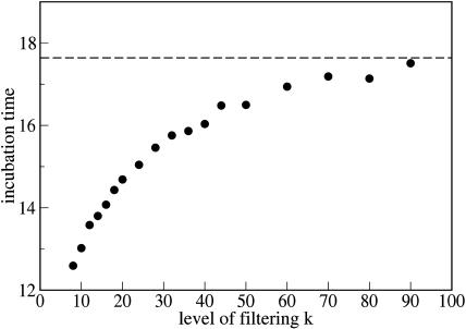
which assures that the initially inoculated mass z(0) does not depend on the degree of filtering k. Fig. 14 shows the incubation time over the degree of filtering. The critical mass of PrP^sc material, i.e., the mass which determines the incubation time, has been chosen as before, z_inc = 2 × 10⁶. As it is seen from Fig. 14 the sickness develops faster if the inoculation consists of shorter PrP^sc aggregates. This effect has a simple explanation: the same amount of the PrP^sc aggregates contains more active ends if it is composed of shorter chains, therefore, the growth occurs more rapidly. For very short molecules, however, when the typical size only slightly exceeds the stable minimum n, one could expect an increase of the incubation time. This may happen, because at the very beginning of the process any splitting of the polymer would lead to its complete disintegration and thus to reduction of the number of growing entities. We do not see the latter effect, however, for the chosen parameters of the simulation.

FIGURE 14.

The incubation time is sensitive to the size distribution of the inoculation. The figure shows the model incubation time over the level of filtering as defined by Eq. 41 for an identical number of PrP^sc units in the inoculation, i.e., for the same value of z(0).

Hence, for experimental purposes, the production of PrP^sc may be enhanced by subdividing long PrP^sc chains into several smaller pieces, e.g., by application of ultrasonic treatment.

COMPARISON WITH EXPERIMENTS

The developed mathematical model can be checked by comparing the theoretical results with available experimental data. As shown above, the assumption of a constant concentration of monomers, being a basic hypothesis of the theory by Masel et al. (1999) and Masel and Jansen (2001), implies qualitatively different scenarios of the disease as compared to the solution of the full set of kinetic equations in Eq. 11 where the concentration of monomers is time-dependent. The comparison with experimental data can discriminate between these scenarios.

The most striking difference between these models is the time-dependence of the number of polymers y(t) (or of the total mass of polymers z(t)). For the simplified model x(t) = x₀, which corresponds to the set of equations Eq. 13, there exist two possible scenarios in dependence on the model parameters: unlimited exponential growth of the number of prion fibrils (i.e., of y(t) or z(t)); or their complete exponential disappearance. The possible scenarios for this simplified model have been illustrated in Fig. 5 (infinite growth) and in Fig. 6 (complete die-off). Contrarily, the solution of the full set of kinetic equations in Eq. 11, i.e., including the time-dependence of the number of monomers, shows initially intensive growth of the number of polymers y(t), but later it saturates at some constant value.

If the onset of clinical disease, or of the death of the infected animal occurred at a time which corresponds to the stage of exponential growth of the number of polymers, it would be difficult to discriminate between the models by means of experimental data. This is definitely the case for Beekes et al. (1996), Taylor et al. (2000), Kimberlin and Walker (1977, 1980, 1986), and Kimberlin et al. (1983), where a linear dependence of the incubation time on the logarithm of the initial dose has been reported.

Fortunately, however, there exist experiments which show saturation of the number of polymers. Rubenstein et al. (1991) infected mice by intracerebral injection as well as by intraperitoneal injection with a mixture of scrapie-associated fibrils (SAFs) of different size. Then the number of the SAFs was directly measured by negative-stain electron microscopy at various times after the inoculation. The details of the infective material and the purification procedure are given by Rubenstein et al. (1991). In these data we clearly observe a saturation of the total mass of the prion polymers—i.e., the data supports our model.

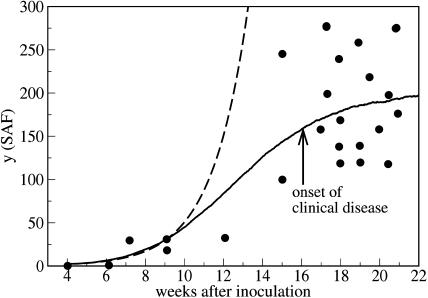
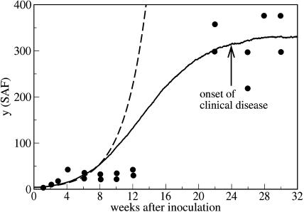
Fig. 15 compares the prediction of our theory with the experimental data given by Rubenstein et al. (1991) for the time-dependent abundance of SAFs after intracerebral inoculation. In Fig. 16 we show the comparison of the theory and experiment for intraperitoneal inoculation. Again we see that the experiment supports the model of variable monomer concentration. This conclusion needs some explanation. First, due to the large scattering of the experimental data, one can also use a nonsaturating curve, which corresponds to the exponential growth. However, the best exponential fit corresponds to a doubling time of ∼25 days which is not consistent with the experimentally observed doubling time. Second, we do not take into account a possible time lag due to spatial propagation of the infective material. For the experimental data shown in Figs. 15 and 16 there is no qualitative difference between the cases of intracerebral and intraperitoneal inoculation. If the time lag was important, one would expect much more pronounced difference between two distinct routes of delivery of the infective material to the spleen. This has been also confirmed by independent measurements of the evolution of the number of PrP^sc polymers in the brain which resembles its evolution in the spleen. The saturation of the curves in this case is clearly visible, too (see Figs. 2 and 3 in Rubenstein et al., 1991).

FIGURE 15.

Time-dependent number of PrP^sc polymers as it follows from the numerical simulation of the set of equations in Eq. 11, including the time-dependence of the number of monomers (full line) together with the experimental data (points) (Rubenstein et al., 1991). The abundance of the fibrils (given in this reference as a number of PrP^sc per a square element of the substrate) was obtained by negative-stain electron microscopy at various times after intracerebral inoculation. The measurements were performed for the spleens of Compton white mice and C57BL/6j mice. The dashed line show the prediction of the simplified model with the same rate constants but with a constant number of monomers, x₀ = λ/d; see Eq. 13. The parameters are n = 6, a = 0.027, b = 4.8 × 10⁻⁴, β = 0.8, λ = 1080, and d = 215.

FIGURE 16.

The same as Fig. 15, but for the intraperitoneal inoculation. The parameters are n = 6, a = 0.018, b = 3.2 × 10⁻⁴, β = 0.32, λ = 1170, and d = 140.

Unfortunately, owing to a lack of any reliable data for the prion size distribution, we cannot compare our theoretical prediction with experiments. Since the model of variable monomer concentration leads to a growth law y(t) which agrees with experimental data, we conclude that this model leads also to the appropriate size distribution function. Hence, we believe that the size distribution of the fibrils is given by Eq. 39 rather than by Eq. 26.

CONCLUSION

Based on the model of Masel et al. (1999) we have derived a mathematically complete set of equations which describes the PrP^sc fibril growth. We analyze these equations both analytically and by means of numerical simulations. First we have considered a simplified set of equations where the number of PrP^c monomers is assumed to be constant (x = const.), i.e., the concentration of monomers is kept constant by regulatory processes in the cell. The full set of kinetic equations for the PrP^sc evolution includes the time-dependence of the monomer concentration, which is determined self-consistently by the rate constants of the system.

We have observed that, depending on the kinetic parameters, there exist several scenarios of the evolution of the disease. For the simplified model (x = const), there are two possible scenarios: unlimited exponential growth of the fibril abundance, or their complete disappearance. Contrarily, for the model of variable number of monomers (x = x(t)), the initial exponential growth of the number of PrP^sc polymers ceases and finally the number of PrP^sc saturates.

We have analyzed the evolution of the distribution of the fibril sizes and obtain analytical expressions for the distribution for both models, x = const and x = x(t). By numerical simulations we have studied the influence of filtering of the inoculation material on the incubation period. Filtering in this sense means to vary the size distribution of the inoculation dose by keeping its total mass z₀ constant. It turns out that the incubation time is very sensitive to the size distribution of the fibrils: keeping the mass of the inoculation constant it can vary by a factor of five when the size distribution varies. This result confirms the importance of filtering in the inoculation and may be checked experimentally.

We compare the prediction of our theory with the available experimental data for the time-dependence of the number of PrP^sc polymers after an inoculation. These experiments strongly support the need to consider the prion fibril growth including the time-dependence of the PrP^c monomer concentration as described by the set of equations in Eq. 11. This model predicts saturation of the number of PrP^sc polymers as compared to unlimited exponential growths for the simplified model where the number of PrP^c monomers is kept constant.

APPENDIX A: NUMERICAL SIMULATIONS

We have simulated the model for PrP^sc polymer kinetics using a numerical method which has been developed independently by Gillespie (1976) and Feistel (1976, 1977). The system can be described as a Markov process, i.e., the transition probability from the present state to a state depends exclusively on the present state but not on the earlier history of the system. The state of the system is characterized by the number y_i of polymers of length i and the number of monomers x, i.e., . If at a certain time the system is in state , this state can be left for any of the following destinations:

1. 

2. 

3. 

4. 

5. 

6. 

7. 

The processes 5–7 correspond to the splitting of a polymer of size m. The rates at which these processes occur depend on the length of the polymer chain m. They are given in Table 1.

TABLE 1.

Process	Rates for m ≥ 2n − 1	Rates for n ≤ m < 2n − 1
(5)	b(m − 2n + 1)ym	0
(6)	2b(n − 1)ym	2b(m − n)ym
(7)	0	b(2n − m − 1)ym
Total	b(m − 1)ym	b(m − 1)ym

A polymer of length m may be cut at m − 1 positions and it was assumed that these cuts occur at equal rate b. Since at state the system contains y_m molecules of size m the total rate of all possible transitions of types 5–7 in which a polymer of size m splits is b(m − 1)y_m (see also discussion of Eq. 3).

For simulations it is sufficient to determine the size m of the polymer which breaks in the next simulation step at rate b(m − 1)y_m due to the algorithm described below. Once m is determined one selects the position of the break, i.e., the final lengths l and k, randomly due to an equidistribution. Depending on their sizes for l < n, k < n these pieces either disintegrate by increasing the number of monomers x or remain stable by increasing the number of polymers y_l, y_k, respectively. This procedure yields precisely the rates which are given in Table 1.

Performing simulation, we have to decide at current time t at what time t + τ the next transition will take place, and what would be the new state among all states which are accessible from by any of the processes of types 1–7.

Assume at time t that the system is in the state . Then p(τ, μ) defines the probability density for the next transition μ to occur in the time interval (t + τ, t + τ + dτ), leading the system to the state , i.e., . This transition probability density factorizes as p(τ, μ) = p₀(τ)p_μ. Here p₀ is the probability for no transition occurring during the time interval (t, t + τ) whereas p_μdτ is the probability that during (t + τ, t + τ + dτ) the state is left via transition μ. In our notations μ belongs to one of the seven types of possible transitions which are listed above, thus, each probability p_μ is determined by the according rates.

From its definition, obviously, p₀(τ) is an exponential distribution

(A1)

where A is the sum of all reaction rates of processes which correspond to transitions , where is any of the states which are accessible by a single transition from . Hence, A is the total rate to leave the present state . For our model A reads

(A2)

In simulations we compute the random value of τ obeying the probability distribution p₀(τ) (Eq. A1) via

(A3)

where RND is an equidistributed random number from the interval (0, 1).

The probability p_μ of the transition μ is determined by

(A4)

where A_μ is the rate of the transition μ. The numerical procedure to determine the transition μ to escape from the present state is sketched in Fig. 17

FIGURE 17.

To choose randomly the transition μ by which the system escapes from the present state we set up an array V containing the cumulative rates, i.e., V[0] = 0, V[1] = V[0] + A₁ = V[0] + λ, V[2] = V[1] + A₂ = V[1] + dx, V[3] = V[2] + A₃ = V[3] + ay_n, etc. Then we draw an equidistributed random number RND from the interval . The process i for which V[i − 1] < RND ≤ V[i] is chosen to be the next process.

.

With these ingredients we can set up an efficient algorithm for the simulation of the system described by the set of equations in Eq. 11. In detail:

1. Initialize the variables x (number of monomers), y_i (number of polymers of size i), and time t = 0.

2. Compute the time τ after which the present state is left according to Eq. A3.

3. Determine the process by which the present state is left as described by Eq. A4 and Fig. 17.

4. Modify the variables x and y_i according to the chosen process.

5. Update the rates A_μ according to the modified variables.

6. Increment time .

7. Extract interesting data, such as , , etc.

8. Continue with step 2.

Simulation techniques of this type have been applied first by Gillespie (1976) and Feistel (1976, 1977).

APPENDIX B: STEADY-STATE DISTRIBUTION OF THE PrP^sc POLYMER SIZES

Assume that the number of monomers is constant and equals x₀. Then the kinetic equation for the numbers of PrP^sc polymers of size i is given by

(B1)

The general solution of this equation reads

(B2)

where the coefficients , B_n, and C_n for i = n, are given by Eq. 23, and for i = n + 1 they may be obtained after the second iterative step,

(B3)

(B4)

(B5)

(B6)

Generally, the coefficient depends on y_n(0), depends on y_n(0) and on y_n+1(0), and depends on y_n(0),…, y_n+l(0).

All terms in Eq. B2 except for the last one decay exponentially, whereas the last one grows exponentially. Thus, after a transient time only this term is nonvanishing. Therefore we may neglect all terms except for the last one and find the solution in the form . Substituting this expression into Eq. B2 we find that the coefficients satisfy the difference equation

(B7)

Now we introduce the quantity

(B8)

so that the initial coefficients C_i may be expressed in terms of Q_i as

(B9)

The equation for the coefficients Q_i reads then as

(B10)

For i ≫ 1 it is reasonable to consider i as a continuous variable, say X and switch from the difference equation in Eq. B10 to the differential equation. Then Q_i − Q_i+1 may be written as −dQ(X)/dX and Q_i+1 − 2Q_i + Q_i−1 as d²Q(X)/dX². In this way we can recast Eq. B10 into the form

(B11)

where

(B12)

Introducing a new variable,

(B13)

we obtain an equation for Q(ξ),

(B14)

which after a substitute Q = W exp(−ξ²/4) yields the equation for the function W(ξ),

(B15)

which is exactly the equation for the harmonic oscillator in quantum mechanics, which is also called the parabolic cylinder equation with index ν = 1 (e.g., Bender and Orzag, 1978). The general solution to this equation is the parabolic cylinder function. For ν = 1 the solution may be expressed through Hermite polynomials,

(B16)

with the constant N to be determined from the boundary conditions. Taking into account that He₁(ξ) = ξ (Bender and Orzag, 1978) and returning to the previously used discrete variable i, we obtain

(B17)

where

(B18)

To find the constant N we notice that after the transient time

(B19)

which yields Q_n = d₁, or

(B20)

where d₁ is determined by the initial conditions. Using Eq. B9 for the coefficients C_i, one can write for the normalized distribution

(B21)

which with Eq. B17 we rewrite in the final form as

(B22)

with

(B23)

as defined previously.

References

- Abramowitz, M., and I. A. Stegun. 1964. Handbook of Mathematical Functions. Dover, New York.
- Alper, T., W. A. Cramp, D. A. Haig, and M. C. Clarke. 1967. Does the agent of scrapie replicate without nucleic acid? Nature. 214:764–766. [DOI] [PubMed] [Google Scholar]
- Beekes, M., E. Baldauf, and H. Diringer. 1996. Sequential appearance and accumulation of pathognomonic markers in the central nervous system of hamsters orally infected with scrapie. J. Gen. Virol. 77:1925–1934. [DOI] [PubMed] [Google Scholar]
- Bender, C., and S. A. Orzag. 1978. Advanced Mathematical Methods for Scientists and Engineers. McGraw-Hill International Editions, Singapore.
- Büeler, H., A. Raeber, A. Sailer, M. Fischer, A. Aguzzi, and C. Weissmann. 1994. High prion and PrPSc levels but delayed onset of disease in scrapie-inoculated mice heterozygous for a disrupted prp gene. Mol. Med. 1:19–30. [PMC free article] [PubMed] [Google Scholar]
- Cohen, F. E., K. M. Pan, Z. Huang, M. Baldwin, R. J. Fletterick, and S. B. Prusiner. 1994. Structural clues to prion replication. Science. 264:530–531. [DOI] [PubMed] [Google Scholar]
- Eigen, M. 1996. Prionics or the kinetic basis of prion diseases. Biophys. Chem. 63:A1–A18. [DOI] [PubMed] [Google Scholar]
- Feistel, R. 1976. Anwendungen der Theorie stochastischer Systeme auf Probleme der Flüssigkeitsphysik. PhD thesis. Wilhelm-Pieck-Universität, Rostock.
- Feistel, R. 1977. Realisierung stochastischer Prozesse. Wiss. Z. Univ. Rostock. 26:663. [Google Scholar]
- Gillespie, D. T. 1976. A general method for numerically simulating the stochastic time evolution of coupled chemical reactions. J. Comput. Phys. 22:403–434. [Google Scholar]
- Griffith, J. S. 1967. Self-replication and scrapie. Nature. 215:1034–1044. [DOI] [PubMed] [Google Scholar]
- Jarrett, J. T., and P. T. Lansbury. 1993. Seeding “one-dimensional crystallization” of amyloid: a pathogenic mechanism in Alzheimer's disease and scrapie? Cell. 73:1055–1058. [DOI] [PubMed] [Google Scholar]
- Jeffrey, M., I. A. Goodbrand, and C. M. Goodsir. 1995. Pathology of the transmissible spongiform encephalopathies with special emphasis on ultrastructure. Micron. 26:277–298. [DOI] [PubMed] [Google Scholar]
- Kimberlin, R. H., H. J. Field, and C. A. Walker. 1983. Pathogenesis of mouse scrapie: evidence for spread of infection from central to peripheral nervous system. J. Gen. Virol. 64:713–716. [DOI] [PubMed] [Google Scholar]
- Kimberlin, R. H., and C. A. Walker. 1977. Characteristics of a short incubation model of scrapie in the golden hamster. J. Gen. Virol. 34:295–304. [DOI] [PubMed] [Google Scholar]
- Kimberlin, R. H., and C. A. Walker. 1980. Pathogenesis of mouse scrapie: evidence for neural spread of infection to the CNS. J. Gen. Virol. 51:183–187. [DOI] [PubMed] [Google Scholar]
- Kimberlin, R. H., and C. A. Walker. 1986. Pathogenesis of scrapie (strain 263K) in hamsters infected intracerebrally, intraperitoneally or intraocularly. J. Gen. Virol. 67:255–263. [DOI] [PubMed] [Google Scholar]
- Lansbury, P. T., and B. Caughey. 1995. The chemistry of scrapie infection: implications of the “ice 9” metaphor. Chem. Biol. 2:1–5. [DOI] [PubMed] [Google Scholar]
- Laplanche, J.-L., N. Hunter, M. Shinagawa, and E. Williams. 1999. Scrapie, chronic wasting disease, and transmissible mink encephalopathy. In Prion Biology and Diseases. S. B. Prusiner, editor. Cold Spring Harbor Laboratory, New York. 393–429.
- Manson, J. C., A. R. Clarke, P. A. McBride, I. McConnell, and J. Hope. 1994. PrP gene dosage determines the timing but not the final intensity or distribution of lesions in scrapie pathology. Neurodegeneration. 3:331–340. [PubMed] [Google Scholar]
- Masel, J., and V. A. A. Jansen. 2001. The measured level of prion infectivity varies in a predictable way according to the aggregation state of the infectious agent. Biochim. Biophys. Acta. 1535:164–173. [DOI] [PubMed] [Google Scholar]
- Masel, J., V. A. A. Jansen, and M. A. Nowak. 1999. Quantifying the kinetic parameters of prion replication. Biophys. Chem. 77:139–152. [DOI] [PubMed] [Google Scholar]
- Parchi, P., R. Castellani, S. Capellari, B. Ghetti, K. Young, S. G. Chen, M. Farlow, D. W. Dickson, A. A. F. Sima, J. Q. Trojanowski, R. B. Petersen, and P. Gambetti. 1996. Molecular basis of phenotypic variability in sporadic Creutzfeldt-Jakob disease. Ann. Neurol. 39:767–778. [DOI] [PubMed] [Google Scholar]
- Prusiner, S. B. 1991. Molecular biology of prion diseases. Science. 252:1515–1522. [DOI] [PubMed] [Google Scholar]
- Prusiner, S. B. 1999a. An introduction to prion biology and diseases. In Prion Biology and Diseases. S. B. Prusiner, editor. Cold Spring Harbor Laboratory, New York. 1.
- Prusiner, S. B. (editor). 1999b. Prion Biology and Diseases. Cold Spring Harbor Laboratory, New York.
- Rubenstein, R., P. A. Merz, R. J. Kascsak, C. L. Scalici, M. C. Papini, R. I. Carp, and R. H. Kimberlin. 1991. Scrapie-infected spleens: analysis of infection, scrapie-associated fibrils, and protease-resistant proteins. J. Infect. Dis. 164:29–35. [DOI] [PubMed] [Google Scholar]
- Scheibel, T., A. S. Kowal, J. D. Bloom, and S. L. Lindquist. 2001. Bidirectional amyloid fiber growth for a yeast prion determinant. Curr. Biol. 11:366–369. [DOI] [PubMed] [Google Scholar]
- Serio, T. R., A. G. Gashikar, A. S. Kowal, G. J. Sawicki, J. J. Moslehi, L. Serpell, M. F. Arnsdorf, and S. L. Lindquist. 2000. Nucleated conformational conversion and replication of conformational information by a prion determinant. Science. 289:1317–1321. [DOI] [PubMed] [Google Scholar]
- Taylor, D. M., I. McConnel, and C. E. Ferguson. 2000. Closely similar values obtained when the ME7 strain of scrapie was titrated in parallel by two individuals in separate laboratories using two sublines of C57BL mice. J. Virol. Methods. 86:35–40. [DOI] [PubMed] [Google Scholar]
- Will, R. G., M. P. Alpers, D. Dormont, L. B. Schonberger, and J. Tateishi. 1999. Infectious and sporadic prion diseases. In Prion Biology and Diseases. S. B. Prusiner, editor. Cold Spring Harbor Laboratory, New York. 465–507.
- Wille, H., M. D. Michelitsch, V. Guenebaut, S. Supattapone, A. Serban, F. E. Cohen, D. A. Agard, and S. B. Prusiner. 2002. Structural studies of the scrapie prion protein by electron crystallography. Proc. Natl. Acad. Sci. USA. 99:3563–3568. [DOI] [PMC free article] [PubMed] [Google Scholar]