Configurational Temperature Density of States Simulations of Proteins

Abstract

A novel method has been implemented to compute the density of states of proteins. A united atom representation and the CHARMM (Brooks et al., 1983) force-field parameters have been adopted for all the simulations. In this approach, an intrinsic temperature is computed based on configurational information about the protein. A random walk is performed in potential energy space and the configurational temperature is collected as a function of potential energy of the system. The density of states is then calculated by integrating the reciprocal of temperature. Unlike previously available methods, this approach does not involve calculations based on histograms of stochastic visits to distinct energy states. It is found that the proposed method is more efficient than earlier, related schemes for simulation of protein folding. Furthermore, it directly provides thermodynamic information, including free energies. The usefulness of the method is discussed by presenting results of simulations of the 16-residue β-hairpin taken from the C-terminal fragment (41–56) of protein G.

INTRODUCTION

Computer simulations of complex systems, including biological molecules, face considerable challenges that are partly attributed to an underlying rough free energy landscape. A system can easily become trapped in local energy minima, thereby precluding adequate sampling of other relevant regions of configurational space. Several advanced Monte Carlo techniques have been proposed to smooth out such landscapes and to provide the resolution required to accurately characterize phase transitions. (Berg and Neuhaus, 1991; Escobedo and de Pablo, 1996; Gront et al., 2000; Hansmann and Okamoto, 1996; Sugita and Okamoto, 2000; Yan and de Pablo, 2000; Yasar et al., 2000). These include parallel tempering, umbrella sampling and multicanonical ensemble techniques. Multicanonical methods (Berg and Neuhaus, 1991) are particularly attractive in that energy barriers can be artificially eliminated by assigning “weights” to different energy states, thereby circumventing some of the problems associated with traditional sampling techniques. The weight factors, however, are not known à priori and their computation often requires tedious iterative calculations.

The central quantity of interest in these simulations is the density of states, Ω(U), which represents the number of accessible states for energy state U of the system. If the density of states is known, efficient algorithms can be constructed to visit distinct energy states with uniform probability, regardless of their location on the energy landscape. Recently, a new class of algorithms (Wang and Landau, 2001a,b) has emerged with the potential of providing a direct estimate of the density of states in a self-consistent manner. Like more established multicanonical algorithms, these methods seek to overcome the problems associated with local free energy barriers. A random walk is performed in energy space to visit distinct energy states. The density of states for each energy state is modified by an arbitrary convergence factor each time a state is visited. A reasonable estimate of Ω(U) is achieved in a self-consistent way by systematically reducing the convergence factor. We have shown recently how this method can be used to study helix-coil and β-sheet-coil transitions of designer peptides on a lattice (Rathore and de Pablo, 2002) and in a continuum (Rathore et al., 2003). Our recent work has also shown (in the context of a simple Lennard-Jones fluid) (Yan and de Pablo, 2003), that the convergence of such methods can deteriorate considerably with the size and complexity of the system. Furthermore, the accuracy of these simulations reaches a stage where additional calculations fail to improve the quality of the results (Yan and de Pablo, 2003).

In this work, a variant of the random walk technique is implemented to study protein folding in a continuum using a united atom representation and the CHARMM19 potential function (Brooks et al., 1983). This new approach is different from earlier algorithms in that a running estimate of Ω(U) is inferred from the instantaneous configurational temperature of the system. It should be contrasted with algorithms in which the density of states is estimated from a histogram of random visits to different energy states. This method has been implemented recently for simulation of a Lennard-Jones fluid (Yan and de Pablo, 2003), where it was shown to be an order of magnitude faster than related algorithms. Given the computational demands of biomolecular simulations in general, it is of considerable interest to pursue a similar implementation in the context of proteins.

We begin with a brief description of the atomistic model, the force field employed in this work, and the β-hairpin fragment of protein G that is used to benchmark the proposed algorithm. We then describe the simulation scheme in detail. A comparison is made between the proposed scheme and Wang and Landau's original method. Results are presented in the form of statistical errors in the estimated density of states.

METHODS

Model

The purpose of this work is to examine the performance of a new algorithm; we therefore restrict our calculations to a system that has been thoroughly characterized in the literature. The C-terminal domain (GEWTYDDATKTFTVTE) of protein G (protein data bank code 1GB1) is used in this work to assess the usefulness of the proposed method. This peptide has been studied extensively by various groups (Dinner et al., 1999; Garcia and Sanbonmatsu, 2001; Lee and Shin, 2001; Pande and Rokhsar, 1999; Zhou et al., 2001) using a variety of force fields and solvent treatments. The consensus from previous work is that it forms a β-hairpin in solution. Thermodynamic and structural studies have shown that this hairpin exhibits many of the basic features of protein folding, including the formation of a hydrophobic core and hydrogen bonds that stabilize the native conformation. Fig. 1 shows a schematic representation of this peptide in its native hairpin configuration.

FIGURE 1.

United atom representation of the native hairpin structure of the C-terminal fragment of protein G.

The CHARMM19 force field is used with a united atom representation where the nonpolar hydrogen atoms are combined with the heavy atoms to which they are bonded. We use the EEF1 model parameters (Lazaridis and Karplus, 1999), where the partial charges on the amino acids are modified to neutralize the side chains and the patched molecular termini. The interactions between atoms are described by the following potential energy function:

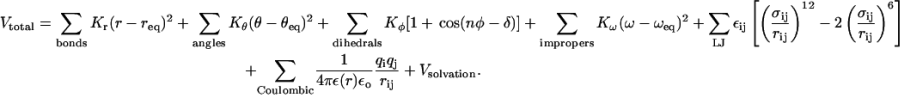(1)

A 1–3 exclusion principle is used for the nonbonded energy. The 1–4 Coulombic interactions are scaled down by a factor of 0.4. This is consistent with the original parameterization of CHARMM19. A cutoff of 12 Å is used for both the electrostatic and van der Waals terms. A force shift scheme is employed for the Coulombic interactions. For Lennard-Jones interactions, a simple cut and shifted potential is employed.

An implicit solvent model based on the solvent accessible surface area (SASA) is employed, with solvation parameters as proposed by Ferrara et al. (2002). Electrostatic screening effects are approximated by a distance dependent dielectric function and a set of partial charges with neutralized side chains. The model assumes that the mean solvation energy is proportional to the SASA of the solute. For a solute having M atoms with Cartesian coordinates r, the solvation term is given by

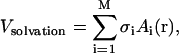(2)

where σ_i and A_i(r) are the atomic solvation parameter and SASA of atom i, respectively. The computations of the atomic solvation parameter and the SASA are performed as indicated in Ferrara et al. (2002). The SASA model, however, only accounts for the free energy cost of burying a charged residue in the interior of a protein. The solvent screening effect is approximated by using a distance-dependent dielectric function, ɛ(r) = r. Although this is an oversimplified way of accounting for solvent polarization effects, it is consistent with the formulation of the SASA model parameters and previous simulations of proteins.

Outline of the method

The internal energy of a system is related to the entropy S and the volume V through

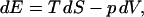(3)

where T is the temperature and p is the pressure. The temperature of the system is related to the density of states Ω(N, V, E) by Boltzmann's equation (McQuarrie, 1976) according to

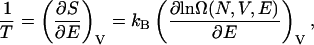(4)

where k_B is Boltzmann's constant. The above equation can be written in terms of the potential energy, U, of the system and integrated to determine the density of states from knowledge of the temperature:

(5)

where Ω(N, V, U) now represents the density of states for an energy state with potential energy, U. Equation 5 requires that the temperature be known as a function of the potential energy. Following our recent work (Yan and de Pablo, 2003), we propose to use the configurational temperature (Butler et al., 1998; Jepps et al., 2000; Rugh, 1997) for this purpose. The details of the original Wang-Landau method and the proposed scheme are provided below.

Wang-Landau density of states (WLDOS)

The random-walk algorithm, as originally proposed by Wang and Landau (Wang and Landau, 2001a,b), has recently been used to study protein folding transitions on a lattice (Rathore and de Pablo, 2002). A slightly modified, more efficient version has also been implemented for simulations of proteins in a continuum (Rathore et al., 2003).

We begin with a brief description of this earlier formalism. The goal of the method is to perform a random walk in energy space with probability proportional to the reciprocal density of states, i.e.,

(6)

If Ω(U) was known with sufficient accuracy, a random walk would lead to flat energy histograms. The density of states however, is not known à priori. In the Wang-Landau method, it is generated “on the fly” as the simulation proceeds. At the beginning of the simulation, Ω(U) is assumed to be unity for all energy states U. Trial Monte Carlo moves are accepted with probability

(7)

where U₁ and U₂ are the energy of the system before and after a trial move. After each trial move, the corresponding density of states is updated by multiplying the current, existing value by a convergence factor f that is greater than unity (f > 1), i.e., Every time that Ω(U) is modified, a histogram of energies H(U) is also updated. This Ω(U) refinement process is continued until H(U) becomes sufficiently flat. Once this condition is satisfied, the convergence factor is reduced by an arbitrary amount. Here we follow Wang and Landau's recommendation and set The energy histogram is then reset to zero (H(U) = 0) and a new simulation cycle is started, continuing until the new histogram H(U) is flat again. The process is repeated until f is smaller than some specified value, e.g., f_final = exp(10⁻⁸). The density of states estimate changes throughout the course of the simulation and detailed balance is not satisfied. Only toward the end of a calculation, when is detailed balance approached. Also, because the value of the convergence factor decreases with the progress of the simulation, configurations generated at different stages of simulation do not contribute equally to the estimated density of states. In fact, toward the final stages of convergence, the convergence factor is so small that the configurations sampled in these stages contribute only negligibly to the final estimate of Ω(U).

Configurational temperature density of states (CTDOS)

An intrinsic temperature, based entirely on configurational information, can be associated with an arbitrary configuration of a system (Jepps et al., 2000) according to

(8)

where subscript i is used to denote a particle, F_i represents the force acting on particle i, and ∇_i = [∂/∂x_i, ∂/∂y_i, ∂/∂z_i] (x_i, y_i, and z_i are the Cartesian coordinates of particle i). This configurational temperature can be particularly helpful in diagnosing programming errors (Butler et al., 1998) in Monte Carlo simulations, where kinetic energy is not explicitly involved.

In the configurational temperature density of states (CTDOS) approach pursued here, temperature is calculated as a function of energy by introducing the above mentioned configurational temperature estimator. For each energy state both the numerator and denominator of Eq. 8 are accumulated separately. Also, histograms are collected for the density of states and potential energy of the system. The total force acting on each particle and the second derivatives of the energy function are evaluated at each step of the simulation, regardless of whether a trial Monte Carlo move is accepted or not. These forces and their derivatives are accumulated and temperature is computed for the current energy state using Eq. 8. At any stage of the simulation two independent estimates of the density of states are therefore available: one computed from the histogram of visited states, and the other from integration of the estimated configurational temperature according to Eq. 5.

In the earlier stages of the simulation, when the convergence factor is large, the detailed balance condition is severely violated. As a result, thermodynamic quantities computed during this time (including the configurational temperature) are incorrect. To avoid carrying this error to later stages, the accumulators for the configurational temperature are reset at the end of early stages, once the density of states has been determined from the current temperature estimate. As the convergence factor decreases (e.g., ln f < 10⁻⁵), the violation of detailed balance has a smaller effect, and the temperature accumulators need not be reset anymore. The dynamic estimate of Ω(U) therefore only serves as a guide to perform the random walk. The actual density of states is computed from the final estimate of configurational temperature, and not from the histogram of visited energy states. All configurations sampled during the simulation now contribute equally to the temperature accumulator, thereby eliminating the problem of nonequal configurational contributions encountered in the original Wang-Landau scheme.

The Monte Carlo algorithm employed here comprises two types of trial moves discussed in detail in previous work (Rathore et al., 2003). Briefly, the first type consists of hybrid molecular dynamics/Monte Carlo displacements; the second type consists of nonlocal pivot attempts. To facilitate convergence and sampling, this implementation is merged with a parallel tempering (or replica exchange) formalism. Multiple noninteracting replicas of the protein molecule are simulated in different boxes. Each simulation box represents an energy window, and the energy ranges in these boxes are assigned so that windows corresponding to adjacent boxes overlap with each other. Configurations in different boxes are swapped at regular intervals during the simulation according to criteria discussed in the literature (Rathore et al., 2003). This ensures that systems in smaller windows do not get trapped in particular configurations as a result of the bounds imposed by the window size.

The main product of the simulation is the density of states over a specified potential energy range, which is determined to within a multiplicative constant. Once Ω(U) is known, thermodynamic quantities such as free energy F(T), internal energy U(T), entropy S(T), and specific heat capacity C(T) can be determined according to:

(9)

(10)

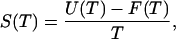(11)

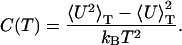(12)

RESULTS AND DISCUSSION

Density of states simulations were performed for the β-hairpin described above (in a continuum solvent). As mentioned earlier, multiple mutually overlapping energy windows were constructed to enhance sampling and facilitate convergence. Fig. 2 a shows the time evolution of potential energy as sampled by each separate box during the course of a simulation. Fig. 2 b shows the accumulated histogram of visited energy states in the overlapping energy windows. Also shown in Fig. 3 are snapshots of instantaneous configurations belonging to different locations of the energy landscape explored by the CTDOS simulation. It is evident from Figs. 2 and 3 that this scheme does facilitate a random walk in energy and configuration space.

FIGURE 2.

(a) Time evolution of potential energy and (b) histogram of visited energy states in different, mutually overlapping energy windows during a CTDOS simulation.

FIGURE 3.

Typical configurations sampled by the peptide during the random walk on the energy landscape. These range from fully folded (a) to completely unfolded (f).

At the end of a simulation, the density of states estimates from different windows can be overlapped and merged to give Ω(U) for the entire energy range of interest. Fig. 4 shows such merged estimates obtained using the two schemes considered here: WLDOS (Wang-Landau) and CTDOS (configurational temperature). It should be noted that Eq. 8 exhibits finite-size effects of order O(1/N). For the β-hairpin considered here, the number of sites is 160, and the error is expected to be of order 10⁻². This small error, however, may accumulate when integrated over a wide energy range and become significant, leading to a systematic error in the CTDOS estimate of Ω(U). Fig. 5 shows the difference between the logarithm of Ω(U) evaluated from a random walk and that determined from configurational temperature in one of the energy windows. The difference is calculated after matching the two ln Ω(U) estimates on the left side of the energy range.

FIGURE 4.

Logarithm of the density of states as obtained from Wang-Landau (WLDOS) and configurational temperature (CTDOS) simulations.

FIGURE 5.

Errors in density of states calculated from CTDOS due to finite-size effects. The solid line represents a least-squares fit: Δ ln Ω(U) = a(U − U_min)² + b(U − U_min), where a = −1.2895 × 10⁻⁶and b = 0.00277.

The discrepancy arising from finite-size effects can be fitted to a quadratic function of the form Δ ln Ω(U) = a(U − U_min)² + b(U − U_min) with a = −1.2895 × 10⁻⁶and b = 0.00277. This simple function provides a means of reducing finite-size effects. We can conduct two preliminary canonical molecular dynamics simulations and get the average potential energy and configurational temperatures. Using linear interpolation we can then compute the systematic error in the ln Ω(U) and subtract it from the estimated value to arrive at a better density of states.

To compare the performance of the original Wang-Landau scheme to the CTDOS method we computed the statistical errors in the two estimates as a function of simulation time. Five independent simulations were conducted with the same code but using different strings of random numbers. The resulting five independent estimates of Ω(U), consistent to within a multiplicative constant, were matched by shifting each ln Ω(U) so as to minimize the total variance. The total variance is given by:

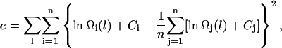(13)

where n is the number of runs (n = 5 for our calculations), l is an index for all energy states, and the constants C_i (or C_j) are the values by which ln Ω(U) is shifted. By minimizing the total variance and by setting C₁ = 0, we get the remaining n − 1 shifting constants. Once the constants are determined, we estimate the statistical error by calculating the standard deviation for each energy state. Fig. 6 shows the statistical errors in the density of states as a function of the convergence factor (f). For the conventional Wang-Landau scheme (represented by solid squares), two different behaviors can be observed, depending on the value of f. For large values of the convergence factor, the error is proportional to the square root of f. But as f gets smaller (ln f < 10⁻⁶), the error approaches a limiting value. Unlike more traditional Monte Carlo algorithms, further simulations do not improve the accuracy of the results. This is because the configurations generated in the late stages of a simulation only contribute negligibly to Ω(U). They only polish the density-of-states estimate locally, but the global estimate remains essentially unchanged. If good sampling and results are not achieved by the time f reaches some threshold value (exp(10⁻⁶) in this case), the final results can be inaccurate.

FIGURE 6.

Statistical error in the density of states as a function of convergence factor (f).

For the configurational temperature method (represented as empty diamonds), the error decreases steadily as the simulation proceeds. For the reasons discussed earlier, the accumulators for the numerator and denominator of Eq. 8 were reset in the early stages (ln f < 10⁻⁵) of the simulation. We therefore see a nonmonotonic behavior for large f. As the convergence factor decreases, the error in the CTDOS estimate becomes progressively smaller. Fig. 7 shows how the statistical errors change with CPU time. We can see that, in contrast to the original WLDOS scheme, CTDOS does not show any asymptotic behavior and the quality of results improves steadily with simulation time. At the end of a simulation, we find that the statistical error from the Wang-Landau scheme is approximately five times as large as that obtained from configurational-temperature calculations.

FIGURE 7.

Statistical error in the density of states as a function of CPU time.

The proposed method exhibits a better performance than that of the Wang-Landau original scheme. This is largely due to the fact that the density of states is computed from the knowledge of configurational information, rather than from a histogram of stochastic visits to distinct energy states. Also, because the proposed scheme involves computing Ω(U) by integrating the estimated temperatures, it eliminates some of the statistical noise involved in these computations. Finally, as discussed earlier, in this method each configuration generated during the simulation contributes equally to the density of states estimate.

Multicanonical methods are particularly useful for characterizing the thermodynamic stability of proteins. Stability can be investigated by introducing mutations in the amino acid sequences and monitoring their effects on transition temperatures and free energy. Other properties including order parameters such as helicity, number of hydrogen bonds or number of native contacts can also be determined efficiently. These methods, however, have not found widespread applications in the study of proteins, partly as a result of the difficulties associated with determining suitable weights for a simulation. One of the attributes of the proposed CTDOS formalism lies in its ability to provide the density of states of a protein in a systematic and self-consistent manner. This attribute of CTDOS will facilitate considerably the application of density-of-states based Monte Carlo methods to the study of biological systems. In this work we have used a complex potential energy function to capture the physics of the folding of a β-hairpin, thereby demonstrating that CTDOS works well with complicated Hessians. Unfortunately, as with other multicanonical techniques, sampling deteriorates for larger systems. However, the finite-size error associated with the configurational temperature decreases as system size increases, providing a more precise estimate of the density of states with increasing system size.

CONCLUSION

A new algorithm to compute the density of states has been applied to simulate the folding of a model protein in a continuum. The method relies on estimating the density of states from the instantaneous configurational temperature of the system. By calculating the gradient of the forces, an intrinsic temperature can be computed and integrated to give the density of states. Unlike earlier techniques based on stochastic visits to energy states, this scheme yields data whose accuracy increases with simulation time.

The configurational temperature does suffer from finite-size effects (of order 1/N). These effects can propagate as 1/T is integrated to generate a density of states. We have shown that by assuming that the finite-size effects are a weak linear function of potential energy, a few preliminary canonical simulations can be used to reduce these systematic errors in the Ω(U) estimate. The CTDOS scheme is expected to work better for larger systems, e.g., peptides in explicit solvents, where finite-size effects in the configurational temperature calculations are expected to be smaller. A detailed study exploring various Wang-Landau schemes for protein systems with explicit water is currently under way.

References

- Berg, B. A., and T. Neuhaus. 1991. Multicanonical algorithms for first order phase transitions. Phys. Lett. B. 267:249–253. [DOI] [PubMed] [Google Scholar]
- Brooks, B. R., R. E. Bruccoleri, B. D. Olafson, D. J. States, S. Swaminathan, and M. Karplus. 1983. CHARMM: A program for macromolecular energy, minimization and dynamics calculations. J. Comput. Chem. 4:187–217. [Google Scholar]
- Butler, B. D., G. Ayton, O. G. Jepps, and D. J. Evans. 1998. Configurational temperature: verification of Monte Carlo simulations. J. Chem. Phys. 109:6519–6522. [Google Scholar]
- Dinner, A. R., T. Lazardis, and M. Karplus. 1999. Understanding β-hairpin formation. Proc. Natl. Acad. Sci. USA. 96:9068–9073. [DOI] [PMC free article] [PubMed] [Google Scholar]
- Escobedo, F. A., and J. J. de Pablo. 1996. Expanded grand canonical and Gibbs ensemble Monte Carlo simulation of polymers. J. Chem. Phys. 105:4391–4394. [Google Scholar]
- Ferrara, P., J. Apostolakiz, and A. Caflisch. 2002. Evaluation of a fast implicit solvent model for molecular dynamics simulations. Proteins. 46:24–33. [DOI] [PubMed] [Google Scholar]
- Garcia, A. E., and K. Sanbonmatsu. 2001. Exploring the energy landscape of a β-hairpin in explicit solvent. Proteins. 42:345–354. [DOI] [PubMed] [Google Scholar]
- Gront, D., A. Kolinski, and J. Skolnick. 2000. Comparison of three Monte Carlo conformational search strategies for a proteinlike homopolymer model: folding thermodynamics and identification of low-energy structures. J. Chem. Phys. 113:5065–5071. [Google Scholar]
- Hansmann, U. H. E., and Y. Okamoto. 1996. Monte Carlo simulations in generalized ensemble: multicanonical algorithm versus simulated tempering. Phys. Rev. E. 54:5863–5865. [DOI] [PubMed] [Google Scholar]
- Jepps, O. G., G. Ayton, and D. J. Evans. 2000. Microscopic expressions for the thermodynamic temperature. Phys. Rev. E. 62:4757–4763. [DOI] [PubMed] [Google Scholar]
- Lazaridis, T., and M. Karplus. 1999. Effective energy function for proteins in solution. Proteins. 35:133–152. [DOI] [PubMed] [Google Scholar]
- Lee, J., and S. Shin. 2001. Understanding β-hairpin formation by molecular dynamics simulations of unfolding. Biophys. J. 81:2507–2516. [DOI] [PMC free article] [PubMed] [Google Scholar]
- McQuarrie, D. A. 1976. Statistical Mechanics. HarperCollins Publishers Inc., New York.
- Pande, V. S., and D. S. Rokhsar. 1999. Molecular dynamics simulations of unfolding and refolding of a β-hairpin fragment of protein G. Proc. Natl. Acad. Sci. USA. 96:9062–9067. [DOI] [PMC free article] [PubMed] [Google Scholar]
- Rathore, N., and J. J. de Pablo. 2002. Monte Carlo simulation of proteins through a random walk in energy space. J. Chem. Phys. 116:7225–7230. [Google Scholar]
- Rathore, N., T. A. Knotts, and J. J. de Pablo. 2003. Density of states simulation of proteins. J. Chem. Phys. 118:4285–4290. [Google Scholar]
- Rugh, H. H. 1997. Dynamical approach to temperature. Phys. Rev. Lett. 78:772–774. [Google Scholar]
- Sugita, Y., and Y. Okamoto. 2000. Replica-exchange multicanonical algorithm and multicanonical replica-exchange method for simulating systems with rough energy landscape. Chem. Phys. Lett. 329:261–270. [Google Scholar]
- Wang, F., and D. Landau. 2001a. Efficient, multiple-range random walk algorithm to calculate the density of states. Phys. Rev. Lett. 86:2050–2053. [DOI] [PubMed] [Google Scholar]
- Wang, F., and D. P. Landau. 2001b. Determining the density of states for classical statistical models: a random walk algorithm to produce a flat histogram. Phys. Rev. E. 64:056101–056116. [DOI] [PubMed] [Google Scholar]
- Yan, Q. L., and J. J. de Pablo. 2000. Hyperparallel tempering Monte Carlo simulation of polymeric systems. J. Chem. Phys. 113:1276–1282. [Google Scholar]
- Yan, Q. L., and J. J. de Pablo. 2003. Fast calculation of the density of states of a fluid by Monte Carlo simulations. Phys. Rev. Lett. 90:035701–035704. [DOI] [PubMed] [Google Scholar]
- Yasar, F., T. Celik, B. A. Berg, and H. Meirovitch. 2000. Multicanonical procedure for continuum peptide models. J. Comput. Chem. 21:1251–1261. [Google Scholar]
- Zhou, R., B. J. Berne, and R. Germain. 2001. The free energy landscape of a β-hairpin folding in explicit water. Proc. Natl. Acad. Sci. USA. 98:14931–14936. [DOI] [PMC free article] [PubMed] [Google Scholar]