Small-World Communication of Residues and Significance for Protein Dynamics

Abstract

It is not merely the position of residues that is critically important for a protein's function and stability, but also their interactions. We illustrate, by using a network construction on a set of 595 nonhomologous proteins, that regular packing is preserved in short-range interactions, but short average path lengths are achieved through some long-range contacts. Thus, lying between the two extremes of regularity and randomness, residues in folded proteins are distributed according to a “small-world” topology. Using this topology, we show that the core residues have the same local packing arrangements irrespective of protein size. Furthermore, we find that the average shortest path lengths are highly correlated with residue fluctuations, providing a link between the spatial arrangement of the residues and protein dynamics.

INTRODUCTION

Proteins are tolerant to mutations with their liquid-like free volume distributions (Baase et al., 1999); however, the average packing density in a protein is comparable to that inside crystalline solids (Tsai et al., 2000). It has been shown that the interiors of proteins are more like randomly packed spheres near their percolation threshold and that larger proteins are packed more loosely than smaller proteins (Liang and Dill, 2001).

At physiological temperatures, the conformational flexibility is essential for biological activity that requires a concerted action of residues located at different regions of the protein (Baysal and Atilgan, 2002; Zaccai, 2000). This cooperation requires an infrastructure that permits a plethora of fast communication protocols. Highly transitive local packing arrangements, giving rise to regular packing geometries (Raghunathan and Jernigan, 1997) cannot provide such short distances between highly separated residues for fast information sharing. On average, random packing of hard spheres similar to soft condensed matter is obtained for a set of representative proteins (Soyer et al., 2000). This architecture is capable of organizing short average path lengths between any two nodes in a structure, but it cannot warrant a high clustering similar to regular packing.

A network is referred to as a small-world network (SWN) if the average shortest path between any two vertices scales logarithmically with the total number of vertices, provided that a high local clustering is observed (Watts and Strogatz, 1998). The former property of short paths is responsible for the name “small world.” Neither regular configurations nor random orientations seem to exhibit these two intrinsic properties that are common in real-world complex networks (Newman, 2000; Strogatz, 2001). Proteins function efficiently, accurately, and rapidly in the crowded environment of the cell; to this end, they should be effective information transmitters by design. With their ordered secondary structural units made up of α-helices and β-sheets on the one hand, and their seemingly unstructured loops on the other, proteins may well have the SWN organization (Vendruscolo et al., 2002).

In this study, we treat proteins as networks of interacting amino acid pairs (Atilgan et al., 2001; Bahar et al., 1997; Yilmaz and Atilgan, 2000). We term these networks as “residue networks” to distinguish them from “protein networks,” which are used to describe systems of interacting proteins (Jeong et al., 2001). We carry out a statistical analysis to show that proteins may be treated within the SWN topology. We analyze the local and global properties of these networks with their spatial location in the three-dimensional structure of the protein. We also show that the shortest path lengths in the residue networks and residue fluctuations are highly correlated.

METHODS

Spatial residue networks

We utilize 595 proteins with sequence homology <25% (Fariselli and Casadio, 1999). We form spatial residue networks from each of these proteins using their Cartesian coordinates reported in the protein data bank (PDB) (Berman et al., 2000). In these networks, each residue is represented as a single point, centered on either the C_α or C_β atoms; in the latter case, C_α atoms are used for glycine residues. Because the general findings of this study are the same irrespective of this choice, we report results from the networks formed of C_β's for brevity. Given the C_β coordinates of a protein with N residues, a contact map can be formed for a selected cutoff radius, r_c, an upper limit for the separation between two residues in contact. This contact map also describes a network that is generated such that if two residues are in contact, then there is a connection (edge) between these two residues (nodes) (Atilgan et al., 2001; Bahar et al., 1997; Yilmaz and Atilgan, 2000). An example network formed for the protein 1ice is shown in Fig. 1. Thus, the elements of the so-called adjacency matrix, A, are given by

(1)

FIGURE 1.

Network construction from a protein. Here the structure of human interleukin 1-β converting enzyme (PDB code: 1ice) is shown on the left. The network constructed from the C^β coordinates of the residues (C^α for Gly) at 7 Å cutoff is shown on the right.

Here, r_ij is the distance between the ith and jth nodes, H(x) is the Heaviside step function given by H(x) = 1 for x > 0 and H(x) = 0 for x ≤ 0.

Network parameters

The networks are quantified by local and global parameters, all of which can be derived from the adjacency matrix. The connectivity k_i of residue i is the number of neighbors of that residue:

(2)

The average connectivity of the network is thus K = 〈k_i〉, where the brackets denote the average.

The characteristic path length, L, of a network is the average over the minimum number of connections that must be transversed to connect residue pair i and j. In computing the shortest path between a pair of nodes, we make use of the fact that the number of different paths connecting a pair of nodes i and j in n steps is given by, . Thus, the shortest path between nodes i and j, L_ij, is given by the minimum power, m, of A for which (A^m)_ij is nonzero. The characteristic path length of the network is the average,

(3)

Note that L is a measure of the global properties, reflecting the overall efficiency of the network.

The clustering coefficient, C, on the other hand, reflects the probability that the neighbors of a node are also neighbors of each other, and as such, it is a measure of the local order. For residue i this probability may be computed by

(4)

Here is the combinatorial coefficient, and k_i is the connectivity as defined in Eq. 2. The clustering coefficient of the network is the average C = 〈C_i〉.

Random rewiring of the residue networks

For comparison purposes, we also generate random networks. The property common to the actual residue network and its random variant is the contact number of a given residue at a fixed cutoff radius. We rewire every residue (node) randomly to another residue chosen from a uniform distribution such that i), it has the same number of neighbors (i.e., k_i and K are the same as the residue network, but C and L change); and ii), the chain connectivity is preserved by keeping the (i, i + 1) contacts intact for all cutoff distances, r_c.

RESULTS

Within the framework of a local interaction network, residues in proteins organize into a SWN topology (see the Appendix for details). Our aim is to study the network topology of residue interactions from a statistical perspective so as to reveal the role of local arrangement on the overall structure and dynamics of proteins. In the rest of this study, we present the results from the residue networks that are constructed using a 7-Å cutoff distance; we have verified that the general conclusions of this work are not affected when an 8.5-Å cutoff distance is used instead.

Connectivity distribution of residues is independent of their spatial location

The connectivity distribution of self-organizing networks has been shown to have direct consequences on the relative weight of i), optimal performance, and ii), tolerance to disturbances of these networks (Newman et al., 2002). At the extreme, scale-free networks are optimal for very fast communication between various parts. They are also very robust toward uncertainties for which they were designed, but are highly vulnerable toward unanticipated perturbations (Carlson and Doyle, 2000). On the other hand, networks may be designed to become more tolerant to attack at the expense of some efficiency, by the utility of broad-scale or single-scale connectivity (Newman et al., 2002). Therefore, the connectivity distribution should also be an indicator of efficiency in proteins.

A plot of the connectivity distribution is displayed in Fig. 2 for the residue networks studied here. We verify that the connectivity distribution of the residue networks constructed at a cutoff distance of 7 Å, which corresponds to the location of the first coordination shell, conform to the Gaussian distribution with a mean of 6.9 Å. It has been suggested that one of the main reasons for deviations from a scale-free connectivity distribution is the limited capacity of a given node (Amaral et al., 2000). In residue networks, this would translate into the excluded volume effect, because the number of residues that can physically reside within a given radius is limited.

FIGURE 2.

Residue contact distribution at r_c = 7 Å, computed as an average over all the residues in a set of 54 proteins. The familiar form of the contact distribution is captured (see, for example, Fig. 4 in Miyazawa and Jernigan, 1996). The contact distributions of core and surface residues are also displayed. Gaussian distribution of coordination numbers is valid for both the hydrophobic core and the molten surface.

Globular proteins may be considered to be made up of a core region surrounded by a molten layer of surface residues. It is of interest to distinguish the topological differences between the core and the surface. Thus, we have also investigated the connectivity distribution of the core and surface residues. We utilize the DEPTH program, which differentiates between such residues by calculating the depth of a residue from the protein surface (Chakravarty and Varadarajan, 1999). We classify the core residues as those residing at depths larger than 4 Å, based on a previous study (Baysal and Atilgan, 2002). We find that the same type of distribution of coordination numbers is valid for both the hydrophobic core and the molten surface, as shown by the separate contact distribution of the surface and core residues (Fig. 2). The means for the respective cases are 5.0 and 8.4 Å. This demonstrates that, the same small-world organization prevails throughout the protein, despite the heterogeneous density distribution.

Clustering of residues is independent of their location in the core

We have further investigated the shortest average path length L_i and the clustering coefficient C_i of residue i as a function of residue depth D_i. For this purpose, we have again used residue depth as a measure of its location in the folded protein. To eliminate the size effect, we have studied a subset of proteins of a fixed number of residues. In Fig. 3, L_i and C_i as a function of residue depth is shown for proteins of size 150 ± 10, 210 ± 10, and 310 ± 10; averages are taken over 24, 15, and 15 proteins in the respective cases.

FIGURE 3.

The depth dependence of the characteristic path length (open symbols) and the clustering coefficient (filled symbols) for proteins of fixed sizes (N = 150: squares, 24 proteins; N = 210: triangles, 15 proteins; N = 310: circles, 15 proteins). The characteristic path length consistently decreases for residues at greater depths; moreover, its value depends on system size. On the other hand, at depths >4 Å, the clustering coefficient attains a fixed value of ∼0.35 irrespective of system size and the location of the residue. Even for the surface residues, the clustering coefficient is independent of system size, although its value is location dependent and somewhat higher than 0.35.

As expected, the shortest path length decreases for residues at greater depths, i.e., those in the core of the protein are connected to the rest of the residues in a fewer number of steps; moreover, this property is size dependent as corroborated by the logarithmic size dependence of the characteristic path lengths (see Fig. 7). Perhaps much less expected, on the other hand, is that the clustering coefficient approaches a fixed value of ∼0.35 beyond a depth of ∼4 Å irrespective of the size of the proteins studied. At greater depths, where the residues are completely surrounded by other residues and are not exposed to the solvent, the local organization of the protein is always the same.

Shortest path lengths and fluctuations are related

Residue fluctuations, which are both experimentally and computationally accessible, provide a rich source of information on the dynamics of proteins around their folded state. It is possible to discern the functionally important motions in proteins using a modal decomposition of the cross-correlations of the fluctuations (Bahar et al., 1998a). Fontana and collaborators have elegantly demonstrated that limited proteolysis, a biochemical method that can be used as a probe of structure and dynamics of both native and partly folded proteins, does not occur at just any site located on the protein surface, but rather shows a good correlation with larger crystallographic B-factors (see Tsai et al., 2002) and references cited therein). Some correlation has also been demonstrated between the residue fluctuations and the native state hydrogen exchange data of folded proteins, the latter providing information on the local conformational susceptibilities of residues (Bahar et al., 1998b).

Thus, repeatedly, residue fluctuations around the folded state emerge as a measurable that can be related to the dynamics of the protein. One would expect an indirect correlation between the fluctuations and shortest path lengths: The former are smaller for highly connected residues, which are in turn connected to the rest of the molecule, on average, in a shorter number of steps. Our analysis on numerous proteins has shown that residue fluctuations are also highly correlated with the shortest path lengths, L_i. In this study residue fluctuations are computed by the Gaussian network model of proteins, which was shown to be in excellent agreement with crystallographic B-factors (Bahar et al., 1999; Baysal and Atilgan, 2001b; Ming et al., 2003). According to this model, average residue fluctuations are given by,. Here Γ is the Kirchoff matrix whose diagonal entries represent the packing density of the ith residue, and the off-diagonal elements are given by the negative of the adjacency matrix elements given by Eq. 1.

Example comparisons between the fluctuations and path lengths are displayed in Fig. 4 for α, β, α + β, and α/β proteins. Note that the correlation that emerges between the fluctuations and path lengths exceeds the expectations from the simple inference outlined above, based on connectivity arguments. Therefore, there is an intriguing balance between these two measurables, one of which (L_i) is more readily associated with the global features and the other (fluctuations) with the local features of the network.

FIGURE 4.

A good correlation between the shortest path lengths (○) and residue fluctuations (•) is observed. Four examples, one of each from α, β, α + β, and α/β class of proteins, are displayed.

An illustrative example of how the SWN perspective supplements biophysical knowledge

CI2 is a model protein that has been extensively studied for understanding protein function, folding, and stability (Fersht, 2000). In Fig. 5, we display how the ideas of shortest path lengths may be applied to gain a better understanding of the processes invoked in response to binding of CI2 to subtilisin novo. Residue Ile-56 of the inhibitor, which is in the binding pocket of the substrate (McPhalen et al., 1985), is shown with its accessible surface. Upon binding, the impact is absorbed by the covalently bonded neighboring residues, Thr-55 and Val-57. The former has noncovalent interactions with Phe-69, and the latter with Arg-67. These two residues are in turn linked to Leu-68. In our earlier work, we have shown that these three residues have the highest capacity of inducing change in the overall protein while resisting perturbations from the rest of the protein (Baysal and Atilgan, 2001a). Considering the size of the impact experienced by the protein upon its interaction with subtilisin novo, which is substantially larger than CI2 (275 residues in the enzyme versus 83 residues in the inhibitor), the energy that is generated upon complexation must be dissipated efficiently and effectively. Thus, this process necessitates fast relaxation through the shortest possible path (small L). Otherwise, small displacements of residues 67–69 will generate relatively large displacements in the rest of the protein, leading to unfolding through a cascade of events. Here, the perturbation is directly communicated to Ala-35 and Ile-76, which have been identified as the stabilizing residues of CI2 (de Prat Gay et al., 1995). With the aid of these stabilizing contacts, a redistribution of the populations of conformations occurs, and the energy landscape is reshaped on the one hand (Kumar et al., 2000; Tsai et al., 1999), and the flexibilities of the residues that are not in direct contact with the substrate is substantially increased, on the other. These tradeoffs help maintain the equilibrium around the native state (Baysal and Atilgan, 2001a). Note that the redistribution path involves the coordination of highly connected residues (contact numbers of Ala-35, Leu-68, and Ile-76 are 11, 10, and 10, respectively) distributed according to a SWN. Note also that the perturbation is propagated to this region through two alternative pathways, creating a redundant link.

FIGURE 5.

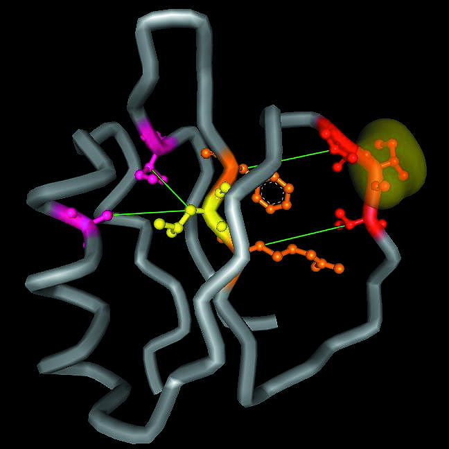
Shortest paths to relieve the impact upon binding of CI2. Ile-56 that is in the binding pocket and that makes many contacts with the substrate, subtilisin novo, is shown with its accessible surface in yellow. Thr-55 and Val-57 (shown in red) are bonded to this residue, and they have their side chains pointing toward the very stable residues of the inhibitor, Arg-67 and Phe-69 (shown in orange). These are in turn connected to the most stable residue of CI2, Leu-68 (shown in yellow). To avoid unfolding, the impact is finally communicated to the stabilizing residues Ala-35 and Ile-76 (shown in purple), which propagate it to the rest of the protein.

CONCLUDING REMARKS

We have shown that the protein structure may be classified as a SWN, balancing efficiency and robustness. We find that the same local organization of core residues appears irrespective of the protein size. Moreover, a remarkable correlation exists between residue fluctuations and shortest path lengths. Recent developments of elastic network models for studying large amplitude motions in proteins have been successful in predicting functional mechanisms (Atilgan et al., 2001; Bahar et al., 1998a, 1999; Keskin et al., 2002). In particular, the cohesive domain-like behavior of proteins is well understood by these models. A similar network construction based on the average structure is used here with a different perspective. Instead of a statistical mechanical approach whereby the system energy is described by the additive local interactions of harmonic springs, a graph theoretical viewpoint is taken by considering pathways of interconnections. That the two approaches, both originating from the packing characteristics, lead to the same information (Fig. 4) calls for further attention.

Most theoretical and computational biophysical methods available today will give information on equilibrium states. The nonequilibrium dynamical information is usually inferred from the study of different equilibrium states and interpolating. The idea of following pathways on networks is an attractive one for studying not-far-from-equilibrium phenomena such as the attainment of new equilibrium states upon binding. However, one first needs to validate the limitations of coarse graining. In particular, the extent to which quantum mechanical effects can be neglected or incorporated into the models must be assessed; e.g., in CO binding to myoglobin (Kriegl et al., 2003) the relaxation pathway in the protein is of utmost interest (Ansari et al., 1985). Consequently, this unifying network perspective will let us explore protein dynamics such that, apart from distinguishing structurally important residues in folding, binding, and stability, we will be able to locate the routes through which a perturbation is communicated in a protein, and estimate the timescales on which a response is generated. As such, it will complement newly developing experimental techniques such as femtosecond spectroscopy (Pal et al., 2002).

The spatiotemporal nature of the hypothesized process calls for deeper investigation on particular proteins. The global rules deduced here for proteins are also expected to have applications in bioinformatics problems such as identifying interaction surfaces in protein docking and distinguishing misfolded states.

APPENDIX: RESIDUES IN PROTEINS ORGANIZE IN A SMALL-WORLD-NETWORK TOPOLOGY

In SWNs, the measure of global communication between any two nodes, characterized by the characteristic path length, L, has the same order of magnitude as a random network. At the same time, the local structure needs to be organized such that the probability that the neighbors of a node are also neighbors of each other is high; in a random network, such a construction does not exist. The latter property is quantified by the clustering coefficient, C (Watts, 1999), which is at least about one order of magnitude larger in SWNs than in their randomized counterparts (Watts and Strogatz, 1998). The final condition for a small-world behavior in a network is that the average path length should scale logarithmically with the total number of vertices (Davidsen et al., 2002). These conditions are summarized as:

(A1)

We first study the ratios L/L_random and C/C_random to understand if the first two of these conditions are met in residue networks. The results are presented in Fig. 6 as a function of the cutoff distance, r_c. We find that L is on the same order as L_random for all values of r_c (right y-axis). For shorter distances (r_c ≤ 8.5 Å) the average path length in real proteins is found to be ∼1.8 times that of random networks; the ratio gradually decreases towards the theoretical limit of 1 as r_c is increased. The clustering coefficient, C, of the residue networks, on the other hand, is ∼9–13 times that of random ones for r_c ≤ 8.5 Å. For larger r_c, the ratio rapidly falls to 1 (left y-axis).

FIGURE 6.

In a SWN, characteristic path length, L, is on the same order of magnitude as its randomized counterpart, whereas clustering density, C, is at least one order of magnitude larger. The variation of the ratios L/L_random (right ordinate) and C/C_random (left ordinate) in the residue networks with the cutoff distance, r_c, used in forming the networks is shown. Note that asr_c → ∞ both L and C approach 1, because every node will be connected to every other node at this limit. (Inset) Radial distribution function of the residue networks. All data are averages over 595 nonhomologous proteins.

The final condition of Eq. A1 for a small-world behavior in a network is that the average path length should scale logarithmically with the total number of vertices (Davidsen et al., 2002). Such a scaling is observed for the proteins studied in this work. A representative case for r_c = 7 Å is shown in Fig. 7. Note that in reproducing this figure, we have clustered the proteins used in this study according to size such that a point corresponding to protein size N corresponds to an average over all proteins in our set that fall in the range N ± 10. Also shown in this figure is the logarithmic scaling of the randomized counterparts of the residue networks. Note that the slope of the latter is 1/log K, a well-known result for Poisson and Gaussian distributed random graphs (Newman et al., 2001).

FIGURE 7.

In a SWN, the characteristic path length, L, should show a logarithmic dependence on the system size, N. Thus, the relation L α log(N) should hold up to a cutoff value of ∼8.5 Å. An example case for r_c = 7 Å is shown. Also shown is the logarithmic dependence of L on N for the randomized networks, the slope of which is the inverse logarithm of the connectivity. That the relationship L = log N/log K should hold for Poisson and Gaussian distributed random networks is a well-known result (Newman et al., 2001).

Thus, interactions within proteins behave like SWNs in the cutoff distance range of up to ∼8.5 Å. We note that Vendruscolo et al. (2002) have studied a set of 978 proteins at a cutoff distance of 8.5 Å with the network perspective. They find that L is 4.1 ± 0.9 and C is 0.58 ± 0.04; they do not show the logarithmic dependence of L on system size, N (last condition in Eq. A1). Nevertheless, based on the small value of the average path length and the relatively large value of the clustering coefficient, they conclude that native protein structures belong to the class of small-world graphs (Vendruscolo et al., 2002), a valid assertion for the 8.5-Å cutoff. To clarify the physical meaning of a cutoff distance in the context of network topology, we look at the radial distribution function for residues in proteins (Fig. 6, inset). Cutoff values of ∼6.5–8.5 Å have been used in studies where coarse graining of proteins is utilized (Bagci et al., 2002; Dokholyan et al., 2002; Miyazawa and Jernigan, 1996). The lower bound corresponds to the first coordination shell of the protein; i.e., the range within which residue pairs are found with the highest probability (6.7 Å for the set used here; first hump in the inset to Fig. 6). A great portion of the contribution to this shell is due to chain connectivity; all (i, i + 1) and most (i, i + 2) pairs fall within this range. Nonbonded residue pairs also exist in this coordination shell. However, the contribution of nonbonded pairs to higher order coordination shells may also be significant (Woodcock, 1997). For C_β–C_β interactions in proteins, the second shell occurs at 8.6 (the second hump in the inset to Fig. 6). Above, we have shown that residues in proteins form small-world networks for the first and second coordination shells. Beyond the second coordination shell the clustering coefficient, C, which is a local property, looses physical significance.

It should be further noted, though, that by reexamining the conditions in Eq. A1 for large proteins, we find that at higher levels of coarse graining, larger cutoffs will again lead to the SWN architecture. We find that L/L_random holds at all cutoff distances (Fig. 6). Similarly, the logarithmic dependence of L on size holds for all cutoff distances studied (r_cut < 30 Å) and similar curves to those in Fig. 7 are obtained. We also find that C/C_random is larger for the larger-sized molecules. For example, the ratio C/C_random is 52, 19, and 9.8 at 7, 10, and 13 Å cutoffs, respectively, for the 996-residue protein 1alo. These numbers are 17, 7.5, and 4.1 at the respective cutoffs for the 250-residue protein 1ctm, representative of the average size of the proteins studied in this work.

The larger (smaller) values of C/C_random for larger (smaller) proteins is due to the following: C is constant in the interior (Fig. 3), and the overall C will fall with N, only due to the decrease in the fraction of surface residues (D < 4.5 Å). This fraction is 0.65, 0.58, and 0.53 for the subgroups of Fig. 3 with protein sizes of 150, 210, and 310 residues, respectively. On the other hand, using well-established results for random graphs; i), C_random = K/N, and ii), K α log(N), the larger the system the smaller C_random. Thus, C decreases less slowly than C_random with the increase in N leading to higher values of C/C_random.

Partial support provided by the Devlet Planlama Teskilati (DPT) Project (grant number 01K120280), Bogazici University Research Foundation Project (grant number 02R102), and Sabanci University Internal Research Grant (grant number A0003-00171) are acknowledged.

References

- Amaral, L. A. N., A. Scala, M. Barthelemy, and H. E. Stanley. 2000. Classes of small-world networks. Proc. Natl. Acad. Sci. USA. 97:11149–11152. [DOI] [PMC free article] [PubMed] [Google Scholar]
- Ansari, A., J. Berendzen, S. F. Bowne, H. Frauenfelder, I. E. T. Iben, T. B. Sauke, E. Shyamsunder, and R. D. Young. 1985. Protein states and protein quakes. Proc. Natl. Acad. Sci. USA. 82:5000–5004. [DOI] [PMC free article] [PubMed] [Google Scholar]
- Atilgan, A. R., S. R. Durell, R. L. Jernigan, M. C. Demirel, O. Keskin, and I. Bahar. 2001. Anisotropy of fluctuation dynamics of proteins with an elastic network model. Biophys. J. 80:505–515. [DOI] [PMC free article] [PubMed] [Google Scholar]
- Baase, W. A., N. C. Gassner, X.-J. Zhang, R. Kuroki, L. H. Weaver, D. E. Tronrud, and B. W. Matthews. 1999. How much sequence variation can the functions of biological molecules tolerate? In Simplicity and Complexity in Proteins and Nucleic Acid. H. Frauenfelder, J. Deisenhofer, and P. G. Wolynes, editors. Dahlem University Press, Berlin, Germany.
- Bagci, Z., R. L. Jernigan, and I. Bahar. 2002. Residue packing in proteins: uniform distribution on a coarse-grained scale. J. Chem. Phys. 116:2269–2276. [Google Scholar]
- Bahar, I., A. R. Atilgan, M. C. Demirel, and B. Erman. 1998a. Vibrational dynamics of folded proteins: significance of slow and fast modes in relation to function and stability. Phys. Rev. Lett. 80:2733–2736. [Google Scholar]
- Bahar, I., A. R. Atilgan, and B. Erman. 1997. Direct evaluation of thermal fluctuations in proteins using a single parameter harmonic potential. Fold. Des. 2:173–181. [DOI] [PubMed] [Google Scholar]
- Bahar, I., B. Erman, R. L. Jernigan, A. R. Atilgan, and D. G. Covell. 1999. Collective dynamics of Hiv-1 reverse transcriptase: examination of flexibility and enzyme function. J. Mol. Biol. 285:1023–1037. [DOI] [PubMed] [Google Scholar]
- Bahar, I., A. Wallqvist, D. G. Covell, and R. L. Jernigan. 1998b. Correlation between native-state hydrogen exchange and cooperative residue fluctuations from a simple model. Biochemistry. 37:1067–1075. [DOI] [PubMed] [Google Scholar]
- Baysal, C., and A. R. Atilgan. 2001a. Coordination topology and stability for the native and binding conformers of chymotrypsin inhibitor 2. Proteins. 45:62–70. [DOI] [PubMed] [Google Scholar]
- Baysal, C., and A. R. Atilgan. 2001b. Elucidating the structural mechanisms for biological activity of the chemokine family. Proteins. 43:150–160. [DOI] [PubMed] [Google Scholar]
- Baysal, C., and A. R. Atilgan. 2002. Relaxation kinetics and the glassiness of proteins: the case of bovine pancreatic trypsin inhibitor. Biophys. J. 83:699–705. [DOI] [PMC free article] [PubMed] [Google Scholar]
- Berman, H. M., J. Westbrook, Z. Feng, G. Gilliland, T. N. Bhat, H. Weissig, I. N. Shindyalov, and P. E. Bourne. 2000. The protein data bank. Nucleic Acids Res. 28:235–242. [DOI] [PMC free article] [PubMed] [Google Scholar]
- Carlson, J. M., and J. Doyle. 2000. Highly optimized tolerance: robustness and design in complex systems. Phys. Rev. Lett. 84:2529–2532. [DOI] [PubMed] [Google Scholar]
- Chakravarty, S., and R. Varadarajan. 1999. Residue depth: a novel parameter for the analysis of protein structure and stability. Structure. 7:723–732. [DOI] [PubMed] [Google Scholar]
- Davidsen, J., H. Ebel, and S. Bornholdt. 2002. Emergence of a small world from local interactions: modeling acquaintance networks. Phys. Rev. Lett. 88:128701. [DOI] [PubMed] [Google Scholar]
- de Prat Gay, G., J. Ruiz-Sanz, J. L. Neira, F. J. Corrales, D. E. Otzen, A. G. Ladurner, and A. R. Fersht. 1995. Conformational pathway of the polypeptide chain of chymotrypsin inhibitor-2 growing from its n terminus in vitro. Parallels with the protein folding pathway. J. Mol. Biol. 254:968–979. [DOI] [PubMed] [Google Scholar]
- Dokholyan, N. V., L. Li, F. Ding, and E. I. Shakhnovich. 2002. Topological determinants of protein folding. Proc. Natl. Acad. Sci. USA. 99:8637–8641. [DOI] [PMC free article] [PubMed] [Google Scholar]
- Fariselli, P., and R. Casadio. 1999. A neural network based predictor of residue contacts in proteins. Protein Eng. 12:15–21. [DOI] [PubMed] [Google Scholar]
- Fersht, A. R. 2000. Transition-state structure as a unifying basis in protein folding mechanisms: contact order, chain topology, stability, and the extended nucleus mechanism. Proc. Natl. Acad. Sci. USA. 97:1525–1529. [DOI] [PMC free article] [PubMed] [Google Scholar]
- Jeong, H., S. P. Mason, A.-L. Barabasi, and Z. N. Oltvai. 2001. Lethality and centrality in protein networks. Nature. 411:41–42. [DOI] [PubMed] [Google Scholar]
- Keskin, O., S. R. Durell, I. Bahar, R. L. Jernigan, and D. G. Covell. 2002. Relating molecular flexibility to function: a case study of tubulin. Biophys. J. 83:663–680. [DOI] [PMC free article] [PubMed] [Google Scholar]
- Kriegl, J. M., K. Nienhaus, P. Deng, J. Fuchs, and G. U. Nienhaus. 2003. Ligand dynamics in a protein internal cavity. Proc. Natl. Acad. Sci. USA. 100:7069–7074. [DOI] [PMC free article] [PubMed] [Google Scholar]
- Kumar, S., B. Ma, C.-J. Tsai, N. Sinha, and R. Nussinov. 2000. Folding and binding cascades: dynamic landscapes and population shifts. Protein Sci. 9:10–19. [DOI] [PMC free article] [PubMed] [Google Scholar]
- Liang, J., and K. A. Dill. 2001. Are proteins well packed? Biophys. J. 81:751–766. [DOI] [PMC free article] [PubMed] [Google Scholar]
- McPhalen, C. A., I. Svendsen, I. Jonassen, and M. N. G. James. 1985. Crystal and molecular structure of chymotrypsin inhibitor 2 from barley seeds in complex with subtilisin novo. Proc. Natl. Acad. Sci. USA. 82:7242–7246. [DOI] [PMC free article] [PubMed] [Google Scholar]
- Ming, D., Y. Kong, Y. Wu, and J. Ma. 2003. Substructure synthesis method for simulation large molecular complexes. Proc. Natl. Acad. Sci. USA. 100:104–109. [DOI] [PMC free article] [PubMed] [Google Scholar]
- Miyazawa, S., and R. L. Jernigan. 1996. Residue-residue potentials with a favorable contact pair term and an unfavorable high packing density term, for simulation and threading. J. Mol. Biol. 256:623–644. [DOI] [PubMed] [Google Scholar]
- Newman, M. E. J. 2000. Models of the small world. J. Stat. Phys. 101:819–841. [Google Scholar]
- Newman, M. E. J., M. Girvan, and J. D. Farmer. 2002. Optimal design, robustness, and risk aversion. Phys. Rev. Lett. 89:028301. [DOI] [PubMed] [Google Scholar]
- Newman, M. E. J., S. H. Strogatz, and D. J. Watts. 2001. Random graphs with arbitrary degree distributions and their applications. Phys. Rev. E 64:026118. [DOI] [PubMed] [Google Scholar]
- Pal, S. K., J. Peon, and A. H. Zewail. 2002. Biological water at the protein surface: dynamical solvation probed directly with femtosecond resolution. Proc. Natl. Acad. Sci. USA. 99:1763–1768. [DOI] [PMC free article] [PubMed] [Google Scholar]
- Raghunathan, G., and R. Jernigan. 1997. Ideal architecture of residue packing and its observation in protein structures. Protein Sci. 6:2072–2083. [DOI] [PMC free article] [PubMed] [Google Scholar]
- Soyer, A., J. Chomilier, J.-P. Mornon, R. Jullien, and J.-F. Sadoc. 2000. Voronoi tessellation reveals the condensed matter character of folded proteins. Phys. Rev. Lett. 85:3532–3535. [DOI] [PubMed] [Google Scholar]
- Strogatz, S. H. 2001. Exploring complex networks. Nature. 410:268–276. [DOI] [PubMed] [Google Scholar]
- Tsai, A. M., D. A. Neumann, and L. N. Bell. 2000. Molecular dynamics of solid-state lysozyme as affected by glycerol and water: a neutron scattering study. Biophys. J. 79:2728–2732. [DOI] [PMC free article] [PubMed] [Google Scholar]
- Tsai, C.-J., P. P. de Laureto, A. Fontana, and R. Nussinov. 2002. Comparison of protein fragments identified by limited proteolysis and by computational cutting of proteins. Protein Sci. 11:1753–1770. [DOI] [PMC free article] [PubMed] [Google Scholar]
- Tsai, C.-J., B. Ma, and R. Nussinov. 1999. Folding and binding cascades: shifts in energy landscapes. Proc. Natl. Acad. Sci. USA. 96:9970–9972. [DOI] [PMC free article] [PubMed] [Google Scholar]
- Vendruscolo, M., N. V. Dokholyan, E. Paci, and M. Karplus. 2002. Small-world view of the amino acids that play a key role in protein folding. Phys. Rev. E 65:061910. [DOI] [PubMed] [Google Scholar]
- Watts, D. J. 1999. Small Worlds. Princeton University Press, Princeton, NJ.
- Watts, D. J., and S. H. Strogatz. 1998. Collective dynamics of “small-world” networks. Nature. 393:440–442. [DOI] [PubMed] [Google Scholar]
- Woodcock, L. V. 1997. Entropy difference between the face-centered cubic and hexagonal close-packed structures. Nature. 385:141–143. [Google Scholar]
- Yilmaz, L. S., and A. R. Atilgan. 2000. Identifying the adaptive mechanism in globular proteins: fluctuations in densely packed regions manipulate flexible parts. J. Chem. Phys. 113:4454–4464. [Google Scholar]
- Zaccai, G. 2000. How soft is a protein? A protein dynamics force constant measured by neutron scattering. Science. 288:1604–1607. [DOI] [PubMed] [Google Scholar]