Restoration of Single-Channel Currents Using the Segmental k-Means Method Based on Hidden Markov Modeling

Abstract

Patch-clamp recording provides an unprecedented means for study of detailed kinetics of ion channels at the single molecule level. Analysis of the recordings often begins with idealization of noisy recordings into continuous dwell-time sequences. Success of an analysis is contingent on accuracy of the idealization. I present here a statistical procedure based on hidden Markov modeling and k-means segmentation. The approach assumes a Markov scheme involving discrete conformational transitions for the kinetics of the channel and a white background noise for contamination of the observations. The idealization is sought to maximize a posteriori probability of the state sequence corresponding to the samples. The approach constitutes two fundamental steps. First, given a model, the Viterbi algorithm is applied to determine the most likely state sequence. With the resultant idealization, the model parameters are then empirically refined. The transition probabilities are calculated from the state sequences, and the current amplitudes and noise variances are determined from the ensemble means and variances of those samples belonging to the same conductance classes. The two steps are iterated until the likelihood is maximized. In practice, the algorithm converges rapidly, taking only a few iterations. Because the noise is taken into explicit account, it allows for a low signal/noise ratio, and consequently a relatively high bandwidth. The approach is applicable to data containing subconductance levels or multiple channels and permits state-dependent noises. Examples are given to elucidate its performance and practical applicability.

INTRODUCTION

Currents flowing through single ionic channels contain valuable information about mechanisms of ion permeation and channel gating. The magnitude of the current indicates the rate of ion flux through the channel, and step changes in the current indicate visible gating kinetics. However, single-channel patch-clamp measurements are invariably contaminated by background noise from a variety of sources including the seal resistance, electronic noise in the amplifier, and shot-noise in the open channel. This noise can be substantial relative to the small current of interest. One of the first stages in the analysis of patch-clamp data is to uncover the underlying single-channel currents, i.e., to idealize the currents so that they appear as they would be in the absence of noise.

Traditionally, single-channel currents are detected by a combination of low-pass filtering and half-amplitude threshold crossing (Sachs et al., 1982; Sigworth, 1983; Gration et al., 1982). Although conceptually simple, these methods suffer from the problem of band-limiting distortions. Because of the small magnitude of the unitary current, heavy filtering is usually necessary so that different conductance levels can be distinguished unambiguously. The finite time response of the low-pass filter, however, may reduce short transitions below threshold and therefore prevent them from being detected. These missed events result in apparent increases in the duration of the experimentally observed dwell times. In the extreme case of small currents with rapid kinetics, the majority of events may be missed. In addition, the noise in the records can either facilitate or depress the detection of individual events, depending on the direction of the noise, and these effects of noise do not cancel out (Blatz and Magleby, 1986). Large noise peaks may be identified as false events.

The threshold crossing techniques incur their limitations in part because of their simplistic assumption that the data points are independent of each other. In reality, the transitions of the channel are time-dependent, and the closed and open samples tend to occur in long runs. Consequently, an improved detection would necessitate the use of information from adjacent samples. Several methods of this type have been developed. For example, Moghaddamjoo (1991) proposed a segmentation procedure in which sequential samples are processed and an event is detected only if the variation of samples within a class is minimized while the variation between classes is maximized. Fredkin and Rice (1992a) introduced two Bayesian restoration methods based on statistical smoothing through the use of a two-state Markov chain. VanDongen and others considered the use of slope threshold in addition to amplitude threshold to minimize spurious transitions (VanDongen, 1996; Tyerman et al., 1992). Nonlinear filtering techniques such as Hinkley detector, which detects abrupt and time-dependent variations, have also been exploited (Draber and Schultze, 1994; Schultze and Draber, 1993). Besides improvements on temporal resolutions, many of these approaches feature a generalized applicability to ion channels with multiple conductance levels, and sometimes even unknown amplitudes.

Hidden Markov modeling (HMM) provides a general paradigm that takes account of the statistical characteristics of both signal and noise simultaneously. The technique has gained popularity in analysis of single-channel currents (Chung et al., 1990; Fredkin and Rice, 1992b; Qin et al., 2000b; Venkataramanan and Sigworth, 2002). Within this framework, channel activity is modeled as a first-order Markov process to which is added white Gaussian noise. The parameters of the model are estimated by maximizing the a priori probability using either the Baum-Welch reestimations or an optimization-based approach (Qin et al., 2000a). The single-channel current is then uncovered as the most likely state sequence by maximizing the a posteriori probability using the Viterbi algorithm (Forney, 1973). Compared to threshold crossing, the approach has a significantly improved detection performance and is particularly well suited for the case in which the signal/noise ratio is poor. However, the maximization of likelihood and the reestimation of parameters are generally a time-consuming process because of the need to evaluate the probability of each state at each sample point. The standard Baum-Welch reestimation requires a computational load that is quadratically proportional to the complexity of the model and linearly to the length of the dataset.

This work extends the study of hidden Markov modeling for single-channel analysis. A simplified HMM approach for idealization of single-channel currents is presented. The approach is based on the segmental k-means (SKM) method (Rabiner et al., 1986). As an alternative to Baum-Welch reestimations, the algorithm is computationally more efficient, thereby alleviating the problem of heavy computations required by the standard HMM. Yet the algorithm maintains the essence of HMM to allow the statistics of both channel kinetics and noise characteristics to be taken into account explicitly in a natural but concise manner. The method, although it estimates models, is intended for idealization of current traces; after this, more sophisticated dwell-time analysis techniques such as histogram fitting or the full dwell-time maximum likelihood approach (Qin et al., 1996, 1997) can be used for model estimation. In the following, the theory of the algorithm is first described. Some issues on implementation and practical use of the algorithm are then addressed. Finally, a number of examples are chosen to demonstrate its performance as well as its limitations.

THEORY

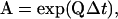
A standard hidden Markov model is used to describe the data. The transitions of the channel are modeled as a Markov process with a discrete number of states, which may refer to the conformations of a protein. The transitions between the states are continuous in time. But in practice, they are observed as discrete samples. Accordingly, a discrete transition probability matrix, namely,

is used to describe the transitions, where the (i,j)^th element a_ij is the probability of making a transition from state i to state j within a sampling interval Δt, and the diagonal element a_ii defines the probability to stay in the current state.

The transition matrix A completely determines the kinetics of the channel, assuming a memoryless system, i.e., the transition at any time is only a function of the current state independent of the previous history. It is related to the rate constant matrix Q by

(1)

where the (i,j)^th element of Q, q_ij, is the rate of transitions from state i to state j, and the diagonal ones are defined so that each row sums to equal zero. Although there is a unique correspondence between the two matrices, the transition probability matrix does not allow specification of disallowed transitions, since its elements generally do not vanish and there is always a chance that the channel may arrive at state j indirectly from state i within a sampling duration even though they are not connected directly. Nevertheless, the sampling interval should be relatively fine to minimize the occurrence of such high-order transitions.

In accordance with observations, each state of the channel is designated with a conductance. Assume a total number of M different conductance levels, and let I_i, i = 1,2…M, be the corresponding current amplitudes. Some of the states may possess an identical conductance. Therefore, there may be more states than conductance levels, i.e., M ≤ N. In the simplest case, there are only two conductance levels, corresponding to closed and open, respectively. However, the model itself is general, without any restriction on the number of subconductance levels. The time series of the observed samples will be denoted by y_t, t = 1…T, and the underlying state sequence by s_t, t = 1…T.

The transitions of the channel are not only masked by aggregation of multiple kinetic states into the same conductance, but also by noise. It is assumed that the noise is additive, white, and follows a Gaussian distribution. The noise can be state-dependent, but for practical consideration, it is only assumed to be conductance-specific. States within the same conductance class have the same noise. By doing so, excessive open noise is allowed. Let σ_i² denote the variance of the noise at the i^th conductance level. Then, given the channel being in conductance i at time t, the resultant observation has a probability distribution

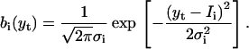(2)

Note that the probability of the observation does not depend on the previous state of the channel or the history of the noise. It is possible to include one previous point within the standard HMM framework. But, an explicit account of the history dependence requires expansion of the state space, which would result in an exponential increase in the computational load.

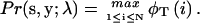
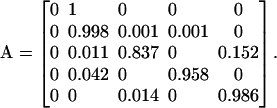
The idealization of the currents can be considered as a restoration problem, i.e., to uncover the underlying state sequence s_t values from the observations y_t values. Apparently, there are many possible solutions, depending on which criterion is used. The idealization considered here is sought to maximize the a posteriori probability of the state sequence, i.e.,

(3)

where λ = {a_ij's, I_i's, σ_i's} designates all model parameters. The probability is also called the likelihood of the idealization.

Making use of the probabilistic model for the channel and the noise, the likelihood can be formulated explicitly. According to the Bayes law, it can be cast into the probability of the state sequence itself, multiplied by the probability observing the samples given that state sequence, leading to

(4)

where the probability of the state sequence Pr(s) is broken into an initial probability π, multiplied by the subsequent transition probabilities through the entire sequence. The problem of idealization is then to choose among all possible choices a state sequence s and a set of model parameters λ so that the probability is maximal.

The problem involves optimization on two categories of unknowns: the state sequence and the model parameters. The first is discrete, although the number of choices may be astronomically large, whereas the second is continuous in values. One approach to the problem is to treat the two types of variables separately and optimize them alternately over each domain,

(5)

That is, the probability is first optimized over s at a fixed model λ and then the state sequence is fixed to optimize the model λ. The first corresponds to idealization of the data with a known model, and the second reestimation of model parameters based on a known idealization along with the given observations.

The idealization of the state sequence given a model is essentially a discrete optimization problem. Given N possible states at each time, there are a total of N^T permutations of state sequences. Since the probability of each sequence can be calculated readily using Eq. 4, it is conceivable to attempt an exhausted search, i.e., to enumerate all state sequences, compare their probabilities, and then determine the one giving the maximal probability. Unfortunately, the strategy is practically unrealistic. Even in the simplest case with two states, there are 2^T sequences for T samples. A small number of 100 samples will result in 10³⁰ state sequences, for which a simple enumeration would take >10²³ years on a computer operating at 1 GHz.

A realistic approach to the problem is the Viterbi algorithm (Forney, 1973), which exploits the unique structure of the problem in combination with the power of dynamic programming (Cormen et al., 1998). The algorithm is recursive and proceeds as follows. Let φ₁(i) = π_ib_i(y₁) for 1 ≤ i ≤ N. Then the following recursion for 2 ≤ t ≤ T and 1 ≤ j ≤ N is

(6)

and

(7)

where i* is a choice of an index i that maximizes φ_t(i). Upon termination, the likelihood is given by

(8)

The most likely state sequence can be recovered from ψ as follows. Let s_T = i*, which maximizes φ_T(i). Then for T ≥ t ≥ 2, s_t−1 = ψ_t(s_t).

The basic idea of the Viterbi algorithm is schematically illustrated in Fig. 1. It performs the idealization through time successively. At each time t, it keeps track of the optimal state sequences (pathways) leading to all possible states at that point. Then, an optimal sequence up to the next time t + 1 is constructed by examining all existing N sequences up to time t in combination with an appropriate transition from time t to t + 1. Because the probabilities of the state sequences up to time t are remembered, the construction of the new extended sequences requires only N² computations, as implied by Eq. 6. The idealization of the entire dataset therefore takes on the order of N²T operations, which is quadratic on the number of states and linear on the number of samples, as opposed to the exponential dependence required by an exhaustive search.

FIGURE 1.

Illustration of the Viterbi algorithm. The optimal sequence leading to a given state at time t + 1 can be constructed from the sequences up to time t combined with a single transition from the previous ending state at time t to the given state at time t + 1.

The result of the Viterbi detection is optimal relative to the model used. In practice, the model is unknown before analysis. As a result, the model parameters need to be estimated. Given an idealization, the estimation can be done empirically. To estimate the current amplitudes and noise variances, one can classify the samples into clusters according to their conductance. The current amplitudes and noise variances can then be estimated as the means and variances of the samples within each cluster, respectively,

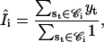(9)

(10)

where 𝒞_i denotes the states of the i^th conductance class, and the denominator represents the number of samples that are idealized into 𝒞_i. Similarly, the transition probability can be estimated by counting the number of transitions occurring from each state, i.e.,

(11)

where n(i) is the number of occurrences of state i and n(i,j) the number of occurrences that state j is an immediate successor of state i.

Ideally, the new estimates of the model parameters should agree with those that initiate the idealization. When the model is unknown, however, they may not be equal, in which case the estimates can be used to upgrade the model. This leads to an iterative loop as shown in Fig. 2, where an initial model, λ₀, is chosen, and the Viterbi algorithm is used to find an optimal idealization from which the model parameters are reestimated. The iteration continues until it converges, for example, when the difference of the parameter values in two consecutive iterations becomes less than a preset small tolerance. This is the essence of the segmental k-means method (Rabiner et al., 1986). Convergence of the algorithm is assured (Juang and Rabiner, 1990), and the reestimated model parameters always give rise to an improved likelihood value at each iteration. As illustrated by examples in the following, the convergence is generally fast, taking only a few iterations.

FIGURE 2.

Block diagram of the SKM algorithm, consisting of two iterative steps, idealization via the Viterbi algorithm and reestimation of model parameters.

IMPLEMENTATION

The segmental k-mean method has a computational load mainly limited by the Viterbi algorithm. The reestimation of model parameters involves only a negligible amount of computation, which is linear on both data length and the number of states. There are several ways to improve the Viterbi algorithm to reduce its complexity. One is to implement the algorithm in the log domain. Instead of calculating φ_t(i), one calculates lnφ_t(i). The recursion Eq. 6 becomes

(12)

which indicates that the log probability lnφ_t(i) can be calculated from its precedent. More importantly, the recursion now involves no multiplication. The algorithm can be implemented with only additions, which is efficient to compute. The use of log probabilities also avoids the problem of numeric overflow. The term φ_t(i) can be considered as a product of probabilities over samples, and if the number of samples is large, the product will eventually exceed the range of computer precision. With the log representation, the problem is avoided.

The other maneuver that can improve the efficiency of the algorithm is to calculate the Gaussian distributions before recursions. This can be done using a lookup table. During recursions, the deviation of a sample from a conductance level can be calculated and discretized to find the appropriate distribution values from the table. This alleviates the expensive computation of exponential functions involved in the distributions.

Application to single-channel currents

The algorithm described above has been tested extensively in the context of idealization of single-channel currents. In the following, a few representative examples are presented. These examples are intended to illustrate the basic performance of the idealization. The algorithm has many features—for example, the allowance for multiple conductance levels or multiple channels, excessive opening noise, constraints on parameters, and so on. The usage of these features is straightforward and will not be discussed here.

The algorithm was implemented in C/C++ language with a Windows graphical interface to support user-interactive manipulations. The interface provides convenient tools for initialization of current amplitudes and noise variances, which are typically “grabbed” from a highlighted region on a data trace. A state model with appropriately specified rate constants is used for initializing the transition probabilities. The program is available through the IcE/QuB software suite (www.qub.buffalo.edu).

Sensitivity to noise and channel kinetics

One advantage of the algorithm is its tolerance for noise. For certain types of channels, good idealization can be achieved at a signal/noise ratio as low as i/σ = 2. As an example, consider the data shown in Fig. 3 A (noisy trace), which were simulated from a two-state model (Scheme I) with current amplitude i = 1 pA and noise standard deviation σ = 0.5 pA. The rate constants of the model were k₁₂ = k₂₁ = 100 s⁻¹. The data were sampled at 100 μs, and a total of 1,000,000 samples were generated. Fig. 3 A (bottom trace) shows the resultant idealization by the algorithm, which agrees well with the true currents, as shown on the top. In total, the simulation resulted in 9967 dwell-times with a mean duration of 10.03 ms. The idealization recovered 9067 events giving a mean duration of 11.03 ms. The error rate of the idealization was therefore within 10% for both the number of events and the mean dwell-time duration. The algorithm was insensitive to the starting values of the model. Repeat of the idealization with different starting values led to comparable results. Fig. 3 B shows the convergence of the log likelihood through iterations. The algorithm generally converged in a few iterations.

FIGURE 3.

An example of idealization. (A) A stretch of data (middle trace) simulated from a two-state model with S/N = 2:1. The clean trace above it was the ideal current before being superimposed with noise. The trace below it was the resultant idealization by the segmental k-mean algorithm. (B) Convergence behavior of the algorithm. The likelihood was normalized by the number of samples. The iterations started at the initial parameter values i = −0.5,1.5; σ = 0.1; and k = 1000 as opposed to their true values i = 0,1; σ = 0.5; and k = 100, respectively. (C) Distribution of occupancy probability of a dense grid of conductance levels uniformly placed between the minimal and the maximal currents. The distribution exhibited two narrow peaks corresponding to the unitary conductance levels of the channel.

SCHEME I.

At a signal/noise ratio of 2:1, the noise from the two conductance levels overlapped significantly. Without a priori knowledge, it is nearly impossible by visual inspection to tell how many conductance levels the channel has or even whether there is channel activity at all, as apparent in Fig. 3. One approach to address such questions is to idealize the data with a sufficient number of conductance levels and then examine the abundance of individual levels. As a test, consider the above data. A set of equally spaced 100 conductance levels were placed from the minimal to the maximal current amplitudes. The algorithm was then applied to segment the data into these preset levels, assuming each level represented a state and transitions occurred only between adjacent levels. From the resultant idealization, the occupancy probability of each level was calculated. Fig. 3 C shows the distribution of these probabilities over all levels. As expected, the distribution exhibited two sharp peaks at positions corresponding to the unitary current amplitudes of the channel. Therefore, even under the condition where the discrete channel activity is concealed by noise, the algorithm is sensitive enough to reveal the presence of the activity. Similar plots of a posterior occupancy probability could be also achieved with the full-likelihood Baum-Welch reestimation procedure (Chung et al., 1990), but the segmental k-means method is more efficient, especially when the model has a high complexity.

Although the algorithm worked well with a noise level as high as σ = 0.5 pA in the above test, this cannot be taken as a general criterion. Its performance also relies on channel kinetics. As the kinetics get fast, the tolerance for noise declines. Fig. 4 A shows the error rates of the idealization as a function of noise level at several kinetic settings. The results were obtained using the same simulation conditions as stated above, except for the rates and noise that were subject to examination. Although the errors were <10% at k × Δt = 0.01 with noise up to σ = 0.55 pA, the same accuracy could only be achieved with σ = 0.35 pA when the kinetics became 10 times faster.

FIGURE 4.

Errors of detections as functions of noise (A) and channel kinetics (B). The increase of noise led to a monotonic degradation on the performance of idealization, whereas the increase of channel kinetics gave rise to biphasic dependence. Rapid kinetics improved detections presumably because of facilitation of noise, as described in the text.

The interplay between kinetics and noise is also evident from Fig. 4 B, which plots the error rates of idealizations as a direct function of kinetics. Interestingly, for a fixed noise level, the error rates of both the number of events and their mean duration showed a biphasic change. The errors increased initially as the kinetics speed up, but it reached a ceiling k × Δt ≈ 0.1, beyond which a further increase of kinetics led to a reduction on the errors. One possible explanation for this biphasic dependence is that with extremely fast kinetics, the correlation between adjacent samples becomes weakened and the channel activity behaves statistically more like a white noise. As a result, the detection of the currents can be actually reinforced by the presence of noise. From the figure, it is evident that the detection degraded rapidly with the increase of either kinetics or noise, consistent with the previous observations in Fig. 4 A.

The algorithm compares favorably with the threshold detection. Fig. 5 shows a direct comparison between the two methods in terms of the number of events and the mean dwell-time duration. As expected, the SKM method exhibits a much higher tolerance for noise. In addition, the erroneous events resulting from SKM appear to be fundamentally different from those obtained with threshold detection. Although the absolute errors of the idealization increase with noise in both cases, they proceed in opposite directions. The SKM method always underestimates the total number of events, whereas the threshold detection overestimates it. Consistently, the mean dwell-time duration is underestimated with SKM but overestimated with threshold. This suggests that the errors involved in SKM idealization are primarily due to missed events whereas threshold detection results in false events. To this extent, the SKM detection is advantageous since the missed events, but not the false events, can be corrected during the stage of dwell-time analysis. To avoid the problem of false events, the threshold analysis has to rely on heavy filtering to minimize errors.

FIGURE 5.

Comparison to threshold detection. The segmental k-means method gave more accurate idealization than the threshold detection as measured by the number of events (A) and the mean dwell-time duration (B). The errors of the idealization also occurred in different directions with the two methods. The segmental k-means method tended to underestimate the number of events and overestimate the mean dwell-time duration. Conversely, the threshold detection led to an excessive number of events with underestimated durations.

It is of interest to know the type of events that may go undetected in the idealization. This information is particularly useful for specification of dead times in dwell-time analysis to correct for the effects of missed events. Fig. 6 shows the distribution of the number of missed events at different durations (in multiples of the sampling duration). The exact distribution varied with kinetics and noise. However, it was common that the missed events at all conditions were predominantly the brief ones, with lifetimes on the order of a few Δt. Furthermore, the distribution appeared to decay exponentially. Beyond 2Δt, the errors reached a plateau and became essentially invariant to kinetics and noise. Therefore, most of the errors arising in the idealization by the algorithm can be attributed to the events with durations <2–3 Δt. This relatively fixed range of missed events offers the possibility for specification of a constant dead time irrespective of underlying channel kinetics or noise level, which is in contrast to threshold detection, where the dead time increases with the level of low-pass filtering.

FIGURE 6.

Distribution of the number of missed events. The algorithm made erroneous detections mostly on the brief events. As the durations of the events increased, the accuracy of their detections was improved exponentially. The errors generally fell off under 10% for durations >2–3 Δt, irrespective of the noise level (A) or the channel kinetics (B).

The SKM detection is not a full maximum likelihood method in the sense that the parameter estimates are not based on a posteriori probability. This raises the question whether the resultant parameter estimates retain the asymptotic properties of the full maximal likelihood estimates such as being efficient and unbiased. Fig. 7 illustrates the deviations of the parameter estimates in the above model as a function of data length, which varied over a range of >100-fold. The plots suggest that the estimates of current amplitudes and noise standard deviation tended to be unbiased, and the variances of the estimates decreased as more samples were included. On the other hand, the kinetic parameters, including both rates and the number of events, exhibited a constant deviation regardless of data length, although their variances decreased too. This suggests that the kinetic estimates given by the algorithm tend to be biased, which is as expected since the estimates are performed empirically and the idealization suffers from omission of brief events.

FIGURE 7.

Asymptotic estimates of model parameters. The estimates of current amplitudes and noise standard deviations appeared to be unbiased and their variances decreased with the length of samples. The number of dwell-times and the rate constants, however, show a constant bias from their true values irrespective of the data length.

Model dependence

This example examines the model dependence of the algorithm. A model for Ca²⁺-activated K⁺ channels (Scheme II) was used (Magleby and Pallotta, 1983). Table 1 lists the values of the rate constants used in simulation. The model has aggregated states, three closed and two open, and the lifetimes of the states span a broad range from tens of milliseconds to submilliseconds. For testing, a total of 1,000,000 samples were simulated, which gave rise to 14,788 dwell-times (16,414 before sampling), with mean closed and open durations of 3.52 and 3.25 ms, respectively. Data was sampled at 50 μs. The unitary current of the channel was 1 pA, and the noise standard deviation σ = 0.25 pA.

SCHEME II.

TABLE 1.

Parameter values for simulation with Scheme II

k12	34	k35	3950
k21	180	k53	322
k23	285	IC	0
k32	600	IO	1
k24	120	σC	0.25
k42	2860	σO	0.25

The simulated data were idealized with models of various topologies. The models examined included the true model (Scheme II), a three-state model (Scheme III), a two-state model (Scheme I), and an uncoupled model (Scheme IV). In all cases, the parameters of the model were subject to reestimation. Table 2 lists some key parameters from the resultant idealizations. With all models, the algorithm accurately recovered the current amplitudes and noise standard deviations, indicating that the estimates of these parameters are independent of model complexity. The reestimates of the dwell-times had a comparable performance among all schemes except for the two-state model. The full model led to 14,054 dwell-times with mean durations τ_C = 3.61 and τ_O = 3.33 ms, which differed from their simulated values by ∼5%. The three-state model, despite its reduced complexity, performed remarkably well; the differences from the full model for both the number of dwell-times and the mean durations were ≤1%. The two-state model, however, showed an error >10%, as compared to the simulated data.

SCHEME III.

SCHEME IV.

TABLE 2.

Results of idealizations obtained with different models for the data simulated using Scheme II

	Scheme II (fixed*)	Scheme II (free†)	Scheme III	Scheme I	Scheme IV
ic	0	−0.02	−0.02	−0.02	−0.02
io	1	0.98	0.98	0.98	0.98
σc	0.25	0.25	0.25	0.25	0.25
σo	0.25	0.25	0.25	0.25	0.25
τc	3.61	3.70	3.68	3.98	3.69
τo	3.33	3.42	3.40	3.68	3.41
Nevent	14,424	14,054	14,110	13,066	14,076

^*Parameters of the model were held at their true values.

^†Parameters of the model were reestimated during idealization.

The testing suggests that the performance of the algorithm does not degrade continuously with the complexity of the model used. Instead, it is relatively insensitive to a wide range of models provided they have a reasonable complexity. The model becomes an issue only when it is over-simplistic and cannot accommodate the major features of the data. In the above example, the data compromised at least two populations of dwell-times with the mean lifetimes separated by about an order of magnitude. Any model of a single closed state is therefore inadequate to represent them. As a consequence, a significant number of events, especially the ones with brief durations, were inevitably missed upon the use of a two-state model.

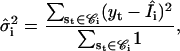
The insensitivity of the algorithm to model topology can also be seen from the reestimates of kinetic parameters. For the full model given above, the transition probability matrix was estimated as

Note that a₁₂ = 1 and a₂₁ = 0, as if the first closed state was absent. This was the case because the lifetimes of C₁ and C₂ were long as opposed to the sampling duration, and collectively they could be represented by a single state. In general, the algorithm performs poorly on the estimation of rates especially between aggregated states, indicating that a model with reduced complexity suffices for a valid idealization.

Since the idealization is the first stage of data analysis, it becomes an issue how to choose a model with adequate complexity. A practical solution to the problem is to develop the model and perform the idealization retrospectively. First, a simplistic model can be used to obtain a relatively coarse idealization. The resulting dwell-time distributions can then be explored for extra components, based on which a model with sufficient complexity can be established. As an example, the data simulated above was first idealized with a two-state model. Fitting of the resultant distributions resolved three closed and two open states. Since the true model topology was unknown, a five-state uncoupled model, as shown in Scheme IV, was used to refine the idealization. A model of this type possessed the maximal complexity for a given number of states that could be possibly resolved for a binary channel based on single-channel measurements (Hui et al., 2003). With the model, the data was reidealized. The results, as shown in Table 2, were improved and became comparable to those obtained with the full model.

Low-pass filtering

In this example, the performance of the algorithm in the presence of low-pass filtering is examined. The two-state model in Scheme I was again used. The simulation conditions were chosen similar to typical experimental settings. The channel had a lifetime of 1 ms for both openings and closures, corresponding to a rate of 1000 s⁻¹. The noise had a standard deviation of σ = 0.5 pA, relative to a 1-pA unitary current. The sampling rate was 50 kHz. A total of 1,000,000 samples were generated. Data were filtered to different extents before idealization. Standard Gaussian digital filters with specified cutoff frequencies were used.

Fig. 8 summarizes the idealization performance as a function of filtering frequency. Also shown are the results from noise-free data to isolate the effect of filtering from that of noise. In the absence of noise, the idealization exhibited a plateau of performance over a wide range of frequency extending from 25 to 5 kHz. Within this range, the error rates on the number of events and the mean dwell-time durations were both <10%. The algorithm started to show significant errors <5 kHz. Further filtering resulted in rapid degradation on idealization. At 1 kHz, the error rate reached nearly 50% for the number of events and >90% for the mean dwell-time duration.

FIGURE 8.

Effect of low-pass filtering. The idealization exhibits a plateau over a wide range of filtering frequency (25–5 kHz) with errors <10% on both the number of events and the mean dwell-time durations. In the absence of noise, the errors increased monotonically (A) with filtering. In the presence of noise, the dependence became biphasic (B), indicating the existence of a filtering frequency for the best idealization performance. The effect of low-pass filtering on idealization by the algorithm is more complex than on the level of noise. The amount of apparent noise decreased more rapidly upon filtering than the idealization errors (C).

The addition of noise complicated the effect of filtering, but did not alter the basic characteristics. Filtering >5 kHz remained to have errors <10%. A notable difference from the noise-free case was that the error rates of the idealization did not increase monotonically with the level of filtering; instead, it peaked ∼10 kHz before entering the rapidly degrading phase. This arose presumably as a result of tradeoff between signal/noise ratio and band-limiting distortions. With little filtering, the noise was high, thereby limiting detections of short events. As filtering increased, the signal/noise ratio improved, and so did the idealization. With further filtering, however, the distortions introduced by low-pass filtering became significant, which caused reduction on the accuracy of the detection again. This biphasic trend suggests that there exists an optimal filtering frequency in practice, although its precise value is less certain pending on the level of noise and the kinetics of the channel.

Application to experimental data

As the final example, the applicability of the algorithm to real experimental data is demonstrated. The data was recorded from a mutant, recombinant mouse n-methyl-d-aspartate (NMDA)-activated receptor expressed in Xenopus oocytes. The recordings were made from outside-out patches (Fig. 9 A, top trace). In these patches, only a single channel was active. The data were digitized at a sampling rate of 20 kHz and low-pass filtered to 10 kHz. A total of 100,000 samples were analyzed. Channel opening is indicated by upward deflection of the signal.

FIGURE 9.

Restoration of single channel currents of a NMDA receptor. (A) A stretch of raw data recorded at 20 kHz and low-pass-filtered to 10 kHz. The recording totaled 100,000 samples (5 s), and only the first 10,000 samples (0.5 s) were shown. The trace below it is the dwell-time sequence produced by the algorithm. The idealization is validated by comparison with the raw data heavily filtered at 1 kHz (bottom trace). (B) The occupancy probability of a set of 30 conductance levels uniformly distributed between the minimal and maximal current amplitudes of the observed data. The distribution reveals three peaks (−7.5, −5, and 0 pA) corresponding to the conductance levels of the channel. (C) The amplitude histogram (jagged contour) superimposed with the theoretical distribution (smooth contour) as constructed from the estimated current amplitudes, noise variances, and occupancy probabilities. The dotted curves are the density for each of the three conductance levels.

The currents appeared to reside at three amplitude levels. Fig. 9 B shows the distribution of the occupancy probability of 30 conductance levels, which were uniformly placed between the minimal (−12 pA) and the maximal (4 pA) current amplitudes. The distribution exhibited three distinct peaks, confirming the existence of a substate. The peaks were located approximately at −7.5, −5, and 0 pA, respectively. Having determined the number and the initial values of conductance levels, the data were reidealized with a nonaggregated three-state model. Fig. 9 A (middle trace) shows the resulting idealization of the data above. Table 3 summarizes the estimated signal statistics.

TABLE 3.

Estimated signal statistics for a NMDA receptor from a record of 100,000 data samples

I (pA)	Occupancy	Lifetime (ms)	Noise SD (pA)
−7.58	0.30	1.89	1.04
−5.05	0.37	1.64	1.04
−0.27	0.33	4.68	0.96

To verify the idealization, the raw data were low-pass-filtered and compared to the restored dwell-time sequence. Fig. 9 A (bottom trace) shows the same data displayed on the top trace but low-pass-filtered at 5 kHz. It is evident that all long events that appeared in the filtered data were successfully restored. Besides, a number of short events, which were visually less obvious from the filtered trace, were also identified. Fig. 9 C shows the all-point amplitude histogram in superimposition with the theoretical distributions that were constructed from the estimated statistics. The overall distribution was in good agreement with the experimental histogram, another indicator suggesting the validity of the idealization.

DISCUSSION

The segmental k-mean method has been explored for the purpose of idealization of single-channel currents. The algorithm relies on probabilistic modeling of data and seeks idealization that has a maximal likelihood. The method has many features that are desirable for single-channel analysis, including its applicability to channels containing subconductance levels and/or state-dependent noises. In particular, the method compares favorably to threshold crossing techniques and allows for a higher level of noise. As such, it extends the limit of the bandwidth at which data can be analyzed and therefore permits extraction of fast kinetics.

The segmental k-means method is closely related to another HMM technique, namely, the Baum-Welch algorithm (Rabiner and Juang, 1986). The latter seeks a model to maximize the probability of the observed samples given the model. Mathematically, this is equivalent to summing up the probability over all possible state sequences. The Baum-Welch algorithm uses the forward-backward procedure to evaluate likelihood and Baum's reestimations to optimize model parameters. Upon determination of the model, a most likely state sequence can be restored using the Viterbi algorithm. The Baum-Welch algorithm is superior to the segmental k-means method as it is a full likelihood approach and produces asymptotically unbiased and efficient estimates of model parameters. The segmental k-means method does not have these properties. But it has the advantage of being computationally efficient. This is particularly true when the Viterbi algorithm is implemented with only addition operations. Furthermore, despite its theoretical inferiority, the method produces adequate idealizations, which are comparable to those obtained with the Baum-Welch algorithm. Therefore, the method can be considered as a good tradeoff between theoretical optimality and practical applicability yet without compromising accuracy of idealization.

The weakness of the segmental k-means method is primarily on its estimation of kinetic parameters of the channel. The method is more sensitive to amplitude variables than to transition probabilities. Examples suggested that the estimates of amplitudes and noise variances are in good agreement with their true values to a good precision. The estimates on kinetic rates, however, tend to be biased when the model has aggregated states. In these cases, the program sometimes simply sets the transition probabilities between aggregated states to zero. This kinetic insensitivity is believed to be a result of the simplistic use of the probability of a single state sequence as the likelihood. The sequence, although most likely, contains only a limited amount of information on the transitions of the channel. In contrast, the Baum-Welch algorithm makes use of both the most likely and less likely sequences, which, collectively, provide a large context of kinetic information. Therefore, a reliable estimation of kinetics requires use of the ultimate full likelihood approach. The estimation of the transitional probabilities resulting from the segmental k-means idealization may be biased.

The relative insensitivity of the segmental k-means method to channel kinetics, on the other hand, provides ease for selection of models. In many cases, a nonaggregated model in which each state corresponds to a conductance level, proved adequate. For binary channels, a simple two-state model may suffice. There are cases where an aggregated model is necessary. This is particularly true when the channel contains dwell-times that are orders-of-magnitude different in durations. Under such conditions, introducing a new state can greatly improve the likelihood as well as idealization, particularly the detection of the fast transitions. In practice, an adequate model can be obtained retrospectively. The data can be first idealized with a relatively simple model. Then the resultant dwell-time distributions can be explored for additional components. Once the number of components is determined, a fully connected and uncoupled model can be used for full idealization. Such a model assures adequate complexity as it has as many parameters as the two-dimensional dwell-time distributions, which are known to contain all the information in the data (Fredkin et al., 1985).

Subsequent analysis of idealized dwell-times requires knowledge of dead time, the minimal duration of the events that can be reliably detected, to correct for effects of missed events. With half-amplitude threshold detection, the dead time is primarily determined by the rise time of the filter. When a Gaussian filter is used, the rise time can be explicitly given as a function of its 3dB cutoff frequency, t_r = 0.3321/f_c (Colquhoun and Sigworth, 1995). The segmental k-means method, on the other hand, does not have such a simple rule. An event is detected not only based on its amplitude but also on its kinetics. A short-lived event may be detected even though its amplitude is under the half-amplitude threshold. This is especially true when the noise is high. Nevertheless, examples suggest that the events that go undetected in the segmental k-mean idealization are mostly the brief ones with duration ≤2Δt. The limit appears to hold for a large range of data with different kinetics and noise levels. Furthermore, the number of missed events appears to decrease exponentially with duration. Therefore, for the dwell-times resulting from the segmental k-means method, the dead time is relatively fixed, intrinsically limited by the method.

The present implementation of the algorithm assumes unfiltered data, to best match the first-order condition of the standard HMM. Despite the assumption, the method is shown to work well with filtered data at a cutoff frequency up to 5 kHz. Over this range, the performance of the idealization remains relatively invariant. Since the method allows for a high level of noise, it generally requires less filtering than this limit for typical patch-clamp data, and therefore is devoid of filtering problems as encountered by other methods such as threshold crossing. For moderately filtered data, it is possible to restore its Nyquist bandwidth with an appropriately designed inverse filter. But for heavily filtered data, the correction is limited. Therefore, it is important to acquire data at a high bandwidth and perform low-pass-filtering offline.

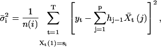
Theoretically, the method can be extended to take account of filtering explicitly. A filtered Markov process exhibits a skewed Gaussian distribution, known as the β-distribution. Therefore, some extent of filtering effect can be taken into account by substituting Gaussian distributions with β-functions. In the paradigm of Markov modeling, it is possible to extend the model to cope with the correlations introduced by filtering. A common practice is to define a meta-state that includes both the current state of the channel and its precious histories (Qin et al., 2000b; Venkataramanan and Sigworth, 2002). If the filter has a response extending over a length of p samples, the meta-states consist of p-tuples as

The distribution of the observations becomes

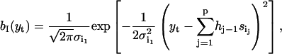(13)

where I = (i₁,i₂,…,i_p)^τ specifies a meta-state and {h_i,1 ≤ i ≤ p} is the impulse response of the filter. The idealization can be done by applying the segmental k-means method to the meta-state Markov process. The reestimations of the current amplitudes and noise variances become

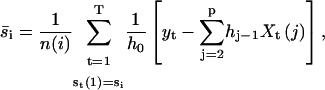(14)

(15)

where n(i) is the number of occurrences of the meta-states in which state i is the first component, and n(i,j) is the number of times to have two consecutive meta-states whose first components are state i and j, respectively. The disadvantage of such high-order modeling is the greatly increased computational load, which is exponential on the length of the filter. Given the insensitivity of the Viterbi detection to the kinetics of the channel, it is unknown how much improvement can be gained in practice with a high-order Markov process.

Although the method has been described in the context of ion channel modeling, it is applicable to other types of single-molecule data as well. Common to all these data is noise contaminating a signal that involves discrete jumps between states. These are essentially the same characteristics of single-channel currents. Therefore, it is anticipated that the method can be used to restore the discrete jumps in these applications. The benefits that have been observed in single-channel analysis, such as the allowance for sublevels and high bandwidths, are expected in those applications as well.

References

- Blatz, A. L., and K. L. Magleby. 1986. Correcting single channel data for missed events. Biophys. J. 49:967–980. [DOI] [PMC free article] [PubMed] [Google Scholar]
- Chung, S. H., J. B. Moore, L. G. Xia, L. S. Premkumar, and P. W. Gage. 1990. Characterization of single channel currents using digital signal processing techniques based on hidden Markov models. Proc. R. Soc. Lond. B Biol. Sci. 329:265–285. [DOI] [PubMed] [Google Scholar]
- Colquhoun, D., and F. J. Sigworth. 1995. Fitting and statistical analysis of single channel records. In Single-Channel Recording. B. Sakmann and E. Neher, editors. Plenum Publishing, New York. 483–587.
- Cormen, T., C. Leiserson, and R. Rivest. 1998. Introduction to Algorithms. The MIT Press, Cambridge, MA.
- Draber, S., and R. Schultze. 1994. Detection of jumps in single-channel data containing subconductance levels. Biophys. J. 67:1404–1413. [DOI] [PMC free article] [PubMed] [Google Scholar]
- Forney, G. D. 1973. The Viterbi algorithm. Proc. IEEE. 61:268–278. [Google Scholar]
- Fredkin, D. R., M. Montal, and J. A. Rice. 1985. Identification of aggregated Markovian models: application to the nicotinic acetylcholine receptor. Proc. Berkeley Conf. in Honor of Jerzy Neymann and Jack Kiefer.
- Fredkin, D. R., and J. A. Rice. 1992a. Bayesian restoration of single-channel patch-clamp recordings. Biometrics. 48:427–448. [PubMed] [Google Scholar]
- Fredkin, D. R., and J. A. Rice. 1992b. Maximum likelihood estimation and identification directly from single-channel recordings. Proc. R. Soc. Lond. B Biol. Sci. 239:125–132. [DOI] [PubMed] [Google Scholar]
- Gration, K. A., J. J. Lambert, R. L. Ramsey, R. P. Rand, and P. N. Usherwood. 1982. Closure of membrane channels gated by glutamate receptors may be a two-step process. Nature. 295:599–603. [DOI] [PubMed] [Google Scholar]
- Hui, K. Y., B. Y. Liu, and F. Qin. 2003. Capsaicin activation of the pain receptor, VR1: multiple open states from both partial and full binding. Biophys. J. 84:2957–2968. [DOI] [PMC free article] [PubMed] [Google Scholar]
- Juang, B. H. and L. R. Rabiner. 1990. The segmental k-means algorithm for estimating parameters of hidden Markov models. IEEE Trans. Acoust. Sp. Sign. Process. 38:1639–1641. [Google Scholar]
- Magleby, K. L., and B. S. Pallotta. 1983. Calcium dependence of open and shut interval distributions from calcium-activated potassium channels in cultured rat muscle. J. Physiol. 344:585–604. [DOI] [PMC free article] [PubMed] [Google Scholar]
- Moghaddamjoo, A. 1991. Automatic segmentation and classification of ionic-channel signals. IEEE Trans. Biomed. Eng. 38:149–155. [DOI] [PubMed] [Google Scholar]
- Qin, F., A. Auerbach, and F. Sachs. 1996. Estimating single channel kinetic parameters from idealized patch-clamp data containing missed events. Biophys. J. 70:264–280. [DOI] [PMC free article] [PubMed] [Google Scholar]
- Qin, F., A. Auerbach, and F. Sachs. 1997. Maximum likelihood estimation of aggregated Markov processes. Proc. R. Soc. Lond. 264:375–383. [DOI] [PMC free article] [PubMed] [Google Scholar]
- Qin, F., A. Auerbach, and F. Sachs. 2000a. A direct optimization approach to hidden Markov modeling for single channel kinetics. Biophys. J. 79:1915–1927. [DOI] [PMC free article] [PubMed] [Google Scholar]
- Qin, F., A. Auerbach, and F. Sachs. 2000b. Hidden Markov modeling for single channel kinetics with filtering and correlated noise. Biophys. J. 79:1928–1944. [DOI] [PMC free article] [PubMed] [Google Scholar]
- Rabiner, L. R., and B. H. Juang. 1986. An introduction to hidden Markov models. IEEE ASSP. 3:4–16. [Google Scholar]
- Rabiner, L. R., J. G. Wilpon, and B. H. Juang. 1986. A segmental k-means training procedure for connected word recognition. AT&T Tech. ET J. 65:21–31. [Google Scholar]
- Sachs, F., J. Neil, and N. Barkakati. 1982. The automated analysis of data from single ionic channels. Pflugers Arch. 395:331–340. [DOI] [PubMed] [Google Scholar]
- Schultze, R., and S. Draber. 1993. A nonlinear filter algorithm for the detection of jumps in patch-clamp data. J. Membr. Biol. 132:41–52. [DOI] [PubMed] [Google Scholar]
- Sigworth, F. 1983. An example of analysis. In Single-Channel Recording. B. Sakmann and E. Neher, editors. Plenum Press, New York. 301–21.
- Tyerman, S. D., B. R. Terry, and G. P. Findlay. 1992. Multiple conductances in the large K+ channel from Chara corallina shown by a transient analysis method. Biophys. J. 61:736–749. [DOI] [PMC free article] [PubMed] [Google Scholar]
- VanDongen, A. M. 1996. A new algorithm for idealizing single ion channel data containing multiple unknown conductance levels. Biophys. J. 70:1303–1315. [DOI] [PMC free article] [PubMed] [Google Scholar]
- Venkataramanan, L., and F. J. Sigworth. 2002. Applying hidden Markov models to the analysis of single ion channel activity. Biophys. J. 82:1930–1942. [DOI] [PMC free article] [PubMed] [Google Scholar]