Cumulant Analysis in Fluorescence Fluctuation Spectroscopy

Abstract

A novel technique for the analysis of fluorescence fluctuation experiments is introduced. Fluorescence cumulant analysis (FCA) exploits the factorial cumulants of the photon counts and resolves heterogeneous samples based on differences in brightness. A simple analytical model connects the cumulants of the photon counts with the brightness ɛ and the number of molecules N in the optical observation volume for each fluorescent species. To provide the tools for a rigorous error analysis of FCA, expressions for the variance of factorial cumulants are developed and tested. We compare theory with experiment by analyzing dye mixtures and simple fluorophore solutions with FCA. A comparison of FCA with photon-counting histogram (PCH) analysis, a related technique, shows that both methods give identical results within experimental uncertainty. Both FCA and PCH are restricted to data sampling times that are short compared to the diffusion time of molecules through the observation volume of the instrument. But FCA theory, in contrast to PCH, can be extended to treat arbitrary sampling times. Here, we derive analytical expressions for the second factorial cumulant as a function of the sampling time and demonstrate that the theory successfully models fluorescence fluctuation data.

INTRODUCTION

Fluorescence fluctuation spectroscopy derives information about biomolecules by measuring the spontaneous intensity fluctuations of fluorescent molecules passing through a small observation volume. Fluorescence fluctuations carry information about transport properties, chemical reactions, and the aggregation state of biomolecules, to name just a few. Statistical analysis techniques are required to unlock the information that is hidden within the experimentally observed fluorescence fluctuations. The most widely used technique, fluorescence correlation spectroscopy (FCS), uses the autocorrelation function to analyze the temporal fluctuations of the fluorescence. FCS has proven extremely powerful for characterizing dynamic processes over timescales from microseconds to seconds (see Hess et al., 2002; Medina and Schwille, 2002; Thompson et al., 2002; Van Craenenbroeck and Engelborghs, 2000, for reviews).

An important aspect of fluorescence fluctuation spectroscopy is the resolution of heterogeneous mixture of biomolecules from analysis of a single measurement. FCS uses the translational diffusion coefficient to separate between different types of molecules. However, if the molecules have similar molecular weights, FCS does not have the sensitivity to separate them (Meseth et al., 1999). An alternative data analysis technique, photon-counting histogram (PCH) analysis, was introduced to overcome this shortcoming of FCS (Chen et al., 1999; Kask et al., 1999).

PCH analysis exploits information from the probability distribution of the photon counts instead of using the autocorrelation function. Thus, PCH and FCS use different information embedded in the noise. PCH distinguishes molecular species by differences in their molecular brightness and not by their diffusion coefficient. For example, assume that two monomeric proteins that are labeled with the same fluorescent dye associate to form a dimer. The dimer carries two fluorescent labels and will appear twice as bright as the monomeric protein. This difference in brightness between the monomer and the dimer allows PCH to separate both species. The resolution of binary mixtures by PCH has been successfully demonstrated (Müller et al., 2000). We recently improved PCH theory (Hillesheim and Müller, 2003) and used it to probe protein interactions in living cells (Chen et al., 2003; Müller, 2003).

The idea that there is more information in the fluorescence fluctuations than used by FCS is not new. Higher order autocorrelation techniques were pioneered by Palmer and Thompson (1987, 1989). A similar approach was taken by Qian and Elson (1990a,b). Both techniques are based on analysis of the higher moments of the photon counts. These techniques were introduced to resolve heterogeneous biomolecule solutions. However, the potential of this approach has not been explored. We will demonstrate that moment analysis is indeed capable of resolving the composition of heterogeneous mixtures. Moreover, we will show that PCH and moment analysis are equally powerful methods for resolving heterogeneous samples. Instead of regular moments we will use cumulants, which are related to moments but have properties particularly useful for fluctuation spectroscopy.

The reasons for developing fluorescence cumulant analysis (FCA) are twofold. First, we want to provide an alternative to PCH analysis. The mathematical description of FCA is rather straightforward and simple to implement in software. In contrast, the PCH algorithm is considerably more sophisticated. Second, cumulant analysis is more flexible than PCH. A substantial amount of theory on cumulants is available. Applying this theory allows the evaluation of cumulants for arbitrary data sampling times. This will allow the expansion of FCA theory to arbitrary sampling times, which will increase the signal statistics of the technique. Here, we will concentrate on the second factorial cumulant of the photon counts and derive expressions for its dependence on the data sampling time. PCH analysis, in contrast to FCA, is restricted to sampling times that are short compared to the diffusion time through the observation volume of the instrument.

We introduce a simple model that expresses cumulants as functions of the brightness ɛ and the number of molecules N for each fluorescent species present. In addition, we formulate and experimentally verify a mathematical model for the statistical error of experimental cumulants. FCA is based on fitting experimental cumulants to theoretical models. Analysis of simple dye mixtures by FCA demonstrates that our theory successfully models the experimental data.

MATERIALS AND METHODS

Instrumentation

Our homebuilt two-photon microscope uses a mode-locked Ti:sapphire laser (Tsunami, Spectra-Physics, Mountain View, CA) pumped by an intracavity doubled Nd:YVO4 laser (Millennia V, Spectra-Physics) as source for two-photon excitation. The laser light passes through a beam expander and enters the modified fluorescence turret of an Axiovert 200 microscope (Carl Zeiss, Thornwood, NY). A 63× Plan Apochromat oil immersion objective (NA = 1.4) was used to focus the light and to collect the fluorescence. For all measurements, an excitation wavelength of 780 nm was used and the average power after the objective was on the order of 6 mW. Under our experimental conditions, no photobleaching was detected for any of the samples measured. Photon counts were detected with an avalanche photodiode (SPCM-AQ-14, PerkinElmer, Dumberry, Québec, Canada). The output of the avalanche photodiode unit, which produces transistor-transistor logic pulses, was directly connected to a data acquisition card (ISS, Champaign, IL). The data acquisition card records the complete sequence of photon counts to computer memory. The data were sampled either at 400 kHz or at 50 kHz. Analysis of the data was performed with programs written for IDL version 5.4 (Research Systems, Boulder, CO).

Sample preparation

Rhodamine 110, Alexa 488, 3-cyano-7-hydroxycoumarin, and fluorescein were purchased from Molecular Probes (Eugene, OR). All dyes were dissolved in 50 mM Tris[hydroxymethy]amino-methane (Sigma, MO) at a pH of 8.5. Dye concentrations were determined by absorption measurements using the extinction coefficients provided by Molecular Probes. Samples for the microscope were prepared by diluting the stock solutions to the desired concentration.

Data analysis

Autocorrelation functions were calculated from the recorded photon counts by software. Photon-counting histogram (PCH) analysis of data was performed as previously described (Müller et al., 2000). PCH determines two parameters for each fluorescent species, the molecular brightness ɛ and the average number of molecules in the excitation volume N. The molecular brightness ɛ is measured in photon counts per sampling time. We used Mathematica (Version 4.1, Wolfram Research, Champaign, IL) and the statistical software package MathStatica (Mathstatica, Sydney, Australia) for deriving the analytical expressions for cumulant analysis. After converting the expressions into computer code, programs written in the IDL language were used for data analysis and for nonlinear least-squares fitting of factorial cumulants. The confidence interval of fit parameters was either determined from the covariance matrix or by F-test analysis (Bevington and Robinson, 1992).

THEORY

Theory of photon detection

Mandel's formula relates the probability distribution function (pdf) p(W) of the integrated light intensity W absorbed by the detector with the pdf p(k) of the photon counts k (Mandel, 1958),

(1)

where Poi(k,x) is the Poisson distribution with an average photon count of x. The parameter η describes the sensitivity of the photo detector, and the intensity I(t) is integrated over the acquisition sampling time T,

(2)

To simplify the equations, we will set η = 1. With this definition, intensity I is measured in photon counts per second (cps), and the integrated intensity W is expressed in units of photon counts. Because of the finite detection sampling time T, we always observe intensity fluctuations of the collected light averaged over the sampling time T. However, if the timescale of the intensity fluctuations is longer than the sampling time T, then the integrated intensity fluctuations track the intensity variations. We will assume that the sampling time T is chosen short enough, so that the fluctuations in W track the intensity fluctuations of interest. This allows us to simplify Eq. 2,

(3)

With this assumption it is possible to calculate the pdf of fluorescence fluctuation experiments for a variety of point spread functions (PSF; Chen et al., 1999). PCH analysis compares the experimentally determined photon-counting histograms with the pdf p(k) of a model. Because PCH theory has been derived under the assumption that Eq. 3 is valid, PCH is only correct for data sampling times T that are short compared to the diffusion time τ_D of molecules through the observation volume. Essentially, the particle is assumed to be stationary (or frozen) during the short sampling period T. The integrated fluorescence intensity of the fluorescent particle only depends on its location r(t) within the PSF,

(4)

The function is the normalized PSF of the instrument (Chen et al., 1999). The parameter ɛ is the brightness of the molecule and depends on the sampling time T,

(5)

where λ is the photon-count rate of a single molecule.

Mandel's formula also relates moments of the integrated intensity with moments of the photon counts. The moment-generating function (mgf) Q_W(s) of the integrated intensities is equal to the factorial mgf of the photon counts (Saleh, 1978), Taking the logarithm of the mgf defines the corresponding cumulant-generating function (cgf). Therefore, the cgf of the integrated intensity is identical to the factorial cgf of the photon counts, Consequently, the r^th integrated intensity cumulants value, κ_r, is equal to the r^th factorial cumulant κ_[r] of the photon counts

(6)

Cumulants are particularly convenient for describing statistically independent variables. Cumulants of the sum of statistically independent variables are simply given by the sum of the cumulants of the individual variables (van Kampen, 1981). The same relationship holds for factorial cumulants. For this reason, fluorescence intensity cumulants scale with the number of molecules in the observation volume, and the corresponding cumulant for a mixture of species is simply given by the sum of the cumulants of each species. All cumulants can be expressed as linear combinations of regular moments (Kendall and Stuart, 1977a). To construct explicit expressions for cumulants in terms of moments, one must derive them from the cgf. For example, the first three cumulants are given by the mean, the variance, and the third central moment, respectively.

Cumulants of fluorescence fluctuation spectroscopy

In fluorescence fluctuation experiments we measure the fluorescence signal from a small illuminated volume. We define an effective observation volume V_PSF by

(7)

where is the normalized PSF with The average number of molecules N in the observation volume V_PSF is proportional to its molar concentration c,

(8)

where N_A is Avogadro's number.

We show in Appendix A that the r^th cumulant of the integrated fluorescence intensity κ_r of diffusing molecules with brightness ɛ is given by

(9)

The coefficients γ_r are defined as by Chen et al. (1999) and Thompson (1991),

(10)

The first two cumulants for a single species are given by

(11)

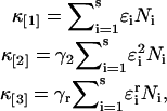
The cumulants for a mixture of s independent species are given by the sum of the cumulants of each species,

(12)

where ɛ_i and N_i are the brightness and number of molecules of species i. Please note that we will often refer in the manuscript to factorial cumulants and regular cumulants simply as cumulants.

Calculation of cumulants and their variances

The factorial cumulants of the photon counts κ_[r] are calculated from the moments of the recorded photon counts. We express factorial cumulants in terms of raw and central moments using moment conversion equations (Kendall and Stuart, 1977a; Rose and Smith, 2002a). The program MathStatica was used for deriving the conversion expressions, which we implemented into our data analysis software. The explicit equations for the first four factorial cumulants in terms of moments of photon counts are

(13)

Expressions of factorial cumulants up to order 10 in terms of moments are also easily constructed using published moment conversion tables (Kendall and Stuart, 1977a).

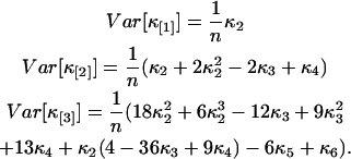
The standard deviation characterizes the experimental uncertainty of factorial cumulants κ_[r] calculated from the raw data. Appendix B shows the steps used for determining the variance of the factorial cumulants. Following this approach, we determined expressions for the variance of the factorial cumulants up to the 10th order with the software package MathStatica. The variance of the first three factorial cumulants expressed in terms of cumulants is given by

(14)

The variance of the factorial cumulants is inversely proportional to the number of data points n sampled as shown in the Appendix. Expressions of the variance for higher order cumulants are of simple polynomial form, but too lengthy to be shown here. We report the variance of the forth and fifth factorial cumulant in Appendix B. We implemented an algorithm into software that determines the variance of the factorial cumulants up to order 10. The algorithm works in two steps. First, we determine the cumulants of the photon counts from the regular photon-count moments using moment-conversion equations (Kendall and Stuart, 1977a). In the second step, we use the cumulants to calculate the variance of the factorial cumulants (see Eq. 14 and Appendix B). We also introduce the relative error and the relative variance which we will use later for describing the statistical uncertainty of fluorescence cumulants.

To perform error analysis we first determine the experimental factorial cumulants κ_[r] from the moments of the photon counts (see Eq. 13). A physical model that specifies the brightness and number of molecules for each species determines the theoretical cumulants κ_[r] according to Eqs. 11 and 12. A nonlinear least-squares optimization program is used for fitting the experimentally determined factorial cumulants k_[r] to the theoretical cumulants κ_[r]. The reduced of the fit is given by

(15)

The value of r₀ is the number of cumulants used in the fit and p is the number of free fitting parameters of the model.

Rebinning of cumulants

Earlier we made the approximation that the data sampling time T is short compared to the characteristic diffusion time of molecules through the observation volume. Now we abandon this approximation and work out the statistics of cumulants for arbitrary data sampling times T. We will restrict ourselves to treating the first two cumulants and Calculating the first cumulant is trivial,

(16)

We exchanged the order of averaging and integration and used the fact that the fluorescence intensity is a stationary process. The first cumulant, which is the average integrated intensity 〈W〉_T, is simply proportional to the sampling time, as expected.

Now, let us calculate the second cumulant, which equals the variance,

(17)

The integrand 〈ΔI(t₁)ΔI(t₂)〉 is proportional to the intensity autocorrelation function,

(18)

The correlation function only depends on the time difference, τ = t₂–t₁, because we are dealing with a stationary process. The autocorrelation function is the product of its amplitude g(0) with a time-dependent factor f(τ), which is model-dependent. The fluctuation amplitude is inversely proportional to the number of particles in the observation volume,

(19)

With these definitions Eq. 17 can be rewritten as

(20)

Here, we transformed the double integral using the fact that the process is stationary. Let us define the binning factor B₂(T),

(21)

The second cumulant can now be written as

(22)

The function B₂(T) describes the dependence of the second cumulant on the data sampling time T. The correlation function of a diffusing species with a two-dimensional Gaussian PSF is given by

(23)

where τ_D is the average diffusion time through the observation volume. The function B₂ for this model is analytically given by

(24)

The correlation function of a diffusing species with a three-dimensional Gaussian PSF is given by

(25)

with r = z₀/ω₀, the ratio of the axial to the radial beam waist of the PSF. The function B₂ for this model is

(26)

We introduced the dimensionless sample time, x = T/τ_D, and the parameter

The influence of finite sampling times on the second moment and correlation functions is well known. The triangular averaging effect of finite sampling times was first considered after the introduction of the multiple tau correlation technique (Schätzel, 1987). The influence of binning for diffusion in the presence of a three-dimensional Gaussian beam profile has been previously treated, and a correction factor that is essentially identical to the binning function B₂(T) shown in Eq. 26 has been introduced (Palo et al., 2000).

RESULTS AND DISCUSSION

Resolving species with cumulants

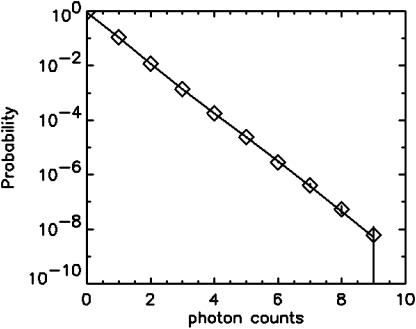
A single fluorescent species is characterized by two parameters, the molecular brightness ɛ and the average number of molecules N. Each cumulant contains unique information not present in cumulants of a different order. In other words, the first two cumulants are sufficient to determine the brightness and average number of molecules in the observation volume. Because analysis of a single species is straightforward, let us consider two species, which is the first nontrivial case. For a binary mixture four cumulants are required to resolve the brightness and average number of molecules for each species. The parameters for a binary mixture can be found analytically by solving the quartic equation that can be constructed from the first four cumulants (Eq. 12). A binary dye mixture of coumarin and rhodamine was mixed in a 70%:30% (v/v) ratio and subsequently measured as outlined in Materials and Methods. Solving the quartic equation leads to the brightness and particle concentration of each species (see Table 1). Analyzing the same data with PCH gives a reduced χ² of 1.2 for a fit of the experimental histogram to a two-species model (Fig. 1). Comparison of the parameters determined from PCH analysis with the results from the cumulant calculation shows very good agreement (Table 1).

TABLE 1.

Analysis of a binary dye mixture

	ɛ1	N1	ɛ2	N2
Cumulants	0.618	0.088	2.076	0.039	—
PCH					1.2
FCA					0.8

Data of a binary dye mixture of coumarin and rhodamine (70%:30% v/v) are analyzed by three different methods: 1), The brightness and the number of molecules of each species are directly computed from the first four factorial cumulants of the photon counts. 2), PCH analysis is used to resolve the binary mixture from the photon-counting histogram. 3), FCA is used to fit the first four factorial cumulants of the photon counts to a two-species model (Eq. 12). The uncertainty of the fit parameters was determined by F-test analysis using a 68% confidence interval.

FIGURE 1.

The PCH function of a binary mixture of rhodamine and coumarin (⋄) is plotted together with an error bar (±σ) for each data point. A fit of the data to a two-species model (solid line) leads to a good description of the experimental histogram. The fit parameters are shown in Table 1.

This experiment demonstrates that two species can be successfully resolved from the first four cumulants. Resolving two species from a single measurement by analysis of photon-count moments has been attempted previously but was not successful (Palmer and Thompson, 1989; Qian and Elson, 1990a). The failure was attributed to insufficient signal statistics. This example illustrates a serious shortcoming of the cumulant approach. Because error analysis of photon-count moments and cumulants was not available, the signal/noise ratio of the experimental data is unknown. We cannot tell if the quality of the data is sufficient to resolve two species. What is worse, even if only a single species is present, calculation of the first four cumulants will still yield parameters for the nonexisting second species. Without error analysis for fluorescence cumulants, we cannot distinguish between different models, nor judge their quality. The advantage of PCH lies in the fact that it provides error analysis. A nonlinear least-squares fit of the experimental histogram assuming a single species leads to a reduced χ² of 217 (data not shown), clearly rejecting the single-species model. To develop a practical analysis tool for cumulants, we need to formulate a theory for the experimental uncertainty of factorial cumulants.

Variance of cumulants

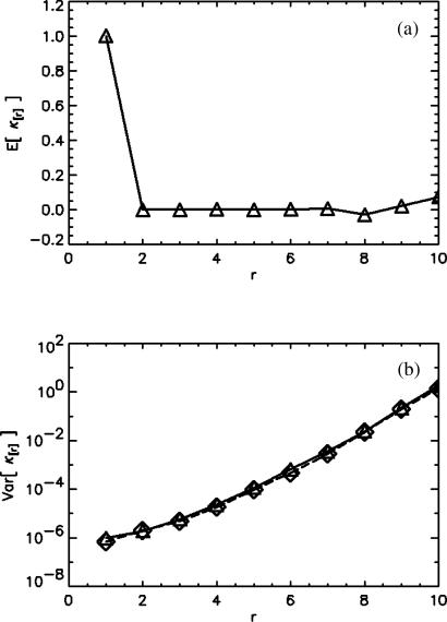
We outlined the theory of error analysis of factorial cumulants in the Theory section. The derivation of the variance of the cumulants is solely based on statistics and therefore valid not only for photon counts but for any random data in general. We used this fact to test our model and its implementation into our analysis software. We generated 100 sets (with 10⁶ data points in each set) of Poisson distributed random data to generate sampling statistics. To characterize the sampling statistics of the factorial cumulants, we determined the expectation value of a factorial cumulant and its variance directly from the 100 sets of data. Fig. 2 a shows the expectation value of the sampling factorial cumulants. Note, that all factorial cumulants κ_[r] with r > 1 vanish for a Poissonian probability distribution function. We also calculate the variance of the factorial cumulants of a single data set by using our theory based on the sampling moments-of-moments technique (Kendall and Stuart, 1977b). Fig. 2 b compares the variance based on the statistics of the 100 simulated data sets with the theoretical variance. The results of both methods are identical and confirm the theoretical approach.

FIGURE 2.

Error analysis of factorial cumulants. A computer generated 100 sets of Poisson distributed random data with 10⁶ data points in each set. The sampling average (▵) and variance (⋄) of the factorial cumulants are shown in a and b. The variance (⋄) was also determined by our theory from a single data set. Both theoretical and experimental variances of the factorial cumulants are in agreement.

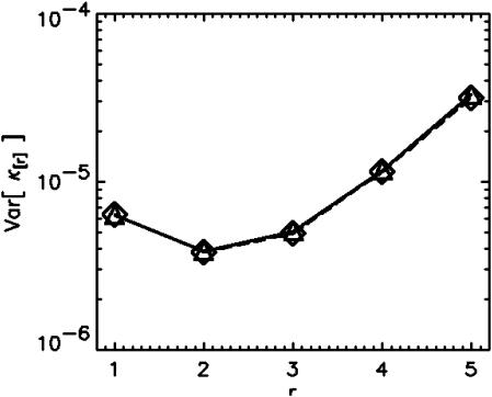
We used the same approach to compare the variances of experimental data. A rhodamine 110 solution was measured for 80 s and the data set was divided into 500 equally sized records. We calculated the sampling variance of the first five cumulants from the 500 records (see triangle in Fig. 3) and compared it with the variance predicted from theory based on the experimental data of a single record (see diamond in Fig. 3). Again, both methods lead to the same result. Because each record contains data taken over the short time period of 0.16 s, we randomly shuffled the data sequence by computer before analysis to destroy the residual correlations between the data of adjacent records.

FIGURE 3.

Error analysis of factorial cumulants. A rhodamine 110 sample was measured for 80 s and subsequently divided into 500 records of equal size. The sampling variance (▵) of the factorial cumulants was determined from the statistics of the 500 records. In addition, the variance was determined from theory based on the data of a single record (⋄). Both theoretical and experimental determination of the variance of the factorial cumulants give the same result.

Fluorescence cumulant analysis

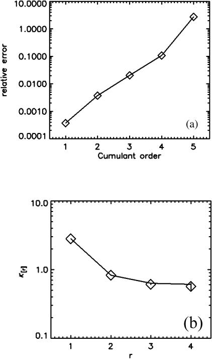
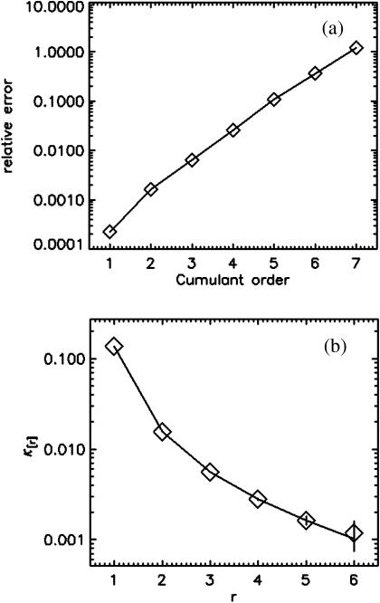
FCA is based on fitting fluorescence cumulants to theoretical models (Eq. 12). The experimental error is calculated from the data (Eqs. 14 and 38), and the quality of the fit is judged by its reduced χ² (Eq. 15). FCA was tested by analyzing data from a fluorescent dye solution (rhodamine 110) taken with a sampling frequency of 50 kHz. A plot of the relative error σ_r in Fig. 4 a reveals that the first four cumulants are statistically significant. A cumulant is considered statistically significant as long as its relative error is <1. We fit the four cumulants to a single-species model and recover fit parameters of ɛ = 3.88 and N = 0.73. Fig. 4 b shows the experimental factorial cumulants and their standard deviation together with the fit. The reduced χ² of the fit is 1.4, which corresponds to a good description of the data by the single-species model.

FIGURE 4.

FCA analysis of a rhodamine 110 sample. (a) The relative error σ_r of the experimental factorial cumulants κ_[r] up to order r = 5. The first four cumulants are statistically significant (σ_r < 1). (b) The experimental cumulants (⋄) are plotted together with an error bar (±σ) for each data point. A fit of the data to a single-species model (solid line) leads to a good description of the experimental histogram. The reduced χ² of the fit is 1.4, and the fit parameters are ɛ = 3.88 and N = 0.73.

Now we reanalyze the 70%:30% (v/v) binary dye mixture of rhodamine and coumarin by FCA (see Table 1). First, we look at the relative error σ_r to determine the number of significant cumulants. The data set contains six significant cumulants (Fig. 5 a). A single-species fit of the first six cumulants leads to a reduced χ² of 236 (data not shown), clearly indicating the need for a different model. A fit of the data to a two-species model describes the experimental cumulants (Fig. 5 b) and results in a reduced χ² of 0.8. The brightness and average number of molecules of both species are shown in Table 1.

FIGURE 5.

FCA analysis of a binary mixture of rhodamine and coumarin. (a) The relative error σ_r of the experimental factorial cumulants κ_[r] up to order r = 7. The first six cumulants are statistically significant (σ_r < 1). (b) The experimental cumulants (⋄) are plotted together with their error bars (±σ). A fit of the data to a two-species model (solid line) leads to a good description of the experimental histogram. The reduced χ² of the fit is 0.8, and the fit parameters are shown in Table 1.

Comparison of FCA with PCH

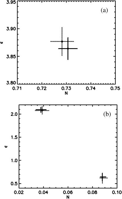
We analyze both a single-species and a two-species sample with PCH and FCA and compare the results. The first sample is a simple rhodamine 110 solution and the second sample is the 70%:30% (v/v) binary mixture of rhodamine 110 and coumarin from Fig. 5. The best-fit parameters are determined by nonlinear-least-squares fitting, and their experimental uncertainty is determined by F-statistics. The reduced χ² for a large number of fits, where one of the parameters is systematically varied, has a minimum if the parameter value equals the best-fit value. We use F-statistics to determine from the χ² function the 68% confidence interval of the fitted parameter, which corresponds to its standard deviation. Fig. 6, a and b, show the fit results together with the uncertainties in fit parameters for both samples. The uncertainties of the fit parameters are also reported in Table 1.

FIGURE 6.

Comparison between FCA and PCH. (a) Data of a fluorescent dye solution are analyzed by PCH and FCA. The best-fit parameters for the brightness and the number of molecules are shown together with their 68% confidence interval (FCA analysis, solid lines; PCH analysis, dotted lines). (b) Data of a binary-dye mixture of rhodamine and coumarin analyzed by PCH and FCA. The best-fit parameters for the brightness and the number of molecules of each species are shown together with their 68% confidence interval (FCA analysis, solid lines; PCH analysis, dotted lines).

The best-fit parameters of both analysis methods are identical within experimental uncertainty. In addition, the standard deviation determined by both techniques is very similar. We have analyzed a large number of data sets and have always found that both analysis techniques give identical results. We conclude that PCH and FCA are equivalent techniques. The absolute brightness values recovered from analysis of the binary dye mixture are consistent with measurements of the brightness of the individual dyes using the same excitation conditions (ɛ₁ = 0.62 for coumarin and ɛ₂ = 2.08 for rhodamine, data not shown). The ratio of the experimental number of molecules is also consistent with the 70%/30% nature of the prepared binary sample.

Rebinning of cumulants

We will examine the theory of the rebinned second cumulant by experiment. For convenience, we define the following function,

(27)

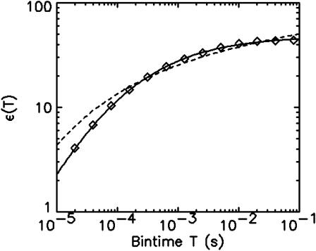
The function ɛ(T) is identical to the molecular brightness at short binning times T. We took data of a rhodamine sample with a sampling frequency of 400 kHz. The brightness function ɛ(T) is shown in Fig. 7 as a function of the bin time T. The data of Fig. 7 are generated as follows: The computer records the photon counts with a sampling time of 2.5 μs and bins the original data by consecutive factors of two. Each binning step simply adds two adjacent photon counts together. This process is equivalent to taking the data with a twice-longer sampling time T for each binning step. The intensity cumulants and are calculated after each step, and the brightness ɛ(T) is graphed as a function of the binning time T. The data in Fig. 7, which are proportional to the molecular brightness, initially increase linearly at short sampling times. This is the regime where PCH theory is correct. At larger sampling times the slope decreases, because molecules are starting to diffuse out of the observation volume. Our theory considers both the brightness and the diffusion time, and thus incorporates aspects of FCS and PCH. This allows us to exploit the brightness at large binning times, where signal statistics is excellent, together with the diffusion time, which determines the shape of the plot in Fig. 7.

FIGURE 7.

Binning of cumulants. Data of a rhodamine sample are successively rebinned by factors of two. The function ɛ(T) (⋄) is calculated from the first two rebinned factorial cumulants (Eq. 27). A fit of the function ɛ assuming a two-dimensional Gaussian beam profile cannot reproduce the experimental data (dashed line). A fit to a model with a three-dimensional Gaussian beam profile describes the data within experimental error (solid line).

A fit of ɛ(T) to a theoretical model assuming a two-dimensional Gaussian excitation profile (Eq. 24) fails to describe the data (Fig. 7). However, a fit of ɛ(T) to a three-dimensional Gaussian model (Eq. 26) describes the experimental data well. The fit determines the molecular photon-count rate (λ = 265 kcps), the diffusion time (τ_D = 18.8 μs), and the aspect ratio of the laser beam profile (r = 5.4). The aspect ratio recovered from the fit is close to 5, which is the value expected for approximating a two-photon Gaussian-Lorentzian beam profile by a three-dimensional Gaussian function (Müller et al., 2003).

DISCUSSION

We introduced a new data analysis technique, factorial cumulant analysis (FCA). Analysis of data by FCA and PCH leads to identical results (Fig. 6). Thus, PCH and FCA are equivalent tools for resolving mixtures of fluorescent molecules from their differences in brightness. This is not surprising, because PCH and FCA are, from a purely mathematical point of view, related. The probability distribution function (pdf) and the cumulant generating function (cgf) contain the same information and can be transformed into one another.

However, there are practical differences between the two techniques. Modeling of PCH functions is complex, whereas FCA analysis offers simple analytical equations that convert models into cumulants (Eq. 12). Thus, implementing algorithms into software is much easier for FCA than it is for PCH.

An advantage of PCH is that although modeling is complex, error analysis is straightforward. Because error analysis for cumulants did not exist, we developed it for factorial photon-count cumulants. Its theory is considerably more complex than that for PCH and requires advanced statistical methods. We constructed analytical solutions for the variance of factorial cumulants up to order 10. The expressions for the first three variances are given in Eq. 14. Although the expressions become lengthy for higher orders, they are given by simple polynomials and are easily implemented into software. Error analysis of factorial cumulants up to order 10 is more than sufficient for fluorescence fluctuation experiments. The number of statistically significant cumulants of our experiments has always been less than eight even for very bright dyes measured at low concentrations.

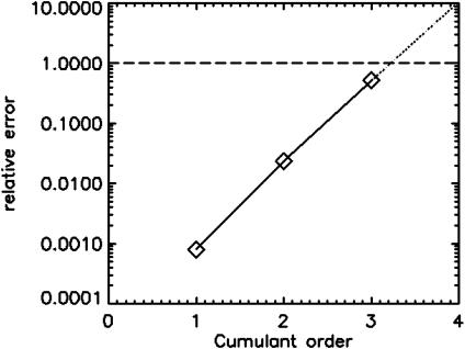
Each fluorescent species requires two cumulants for the determination of its brightness and its number of molecules. In other words, 2n statistically significant cumulants are necessary for resolving a mixture of n species. But how many experimental factorial cumulants of a given data set are reliable? FCA provides a straightforward way to answer this question by evaluating the relative error of the experimental cumulants. The relative error of the cumulants increases as a function of its order (see Fig. 5 a). Only values with a relative error of <1 are acceptable for data analysis. This provides a very convenient check to see if the statistical accuracy of the data is sufficient for resolving species. For example, Fig. 8 shows the relative error of the factorial cumulants for a mixture of rhodamine 110 and coumarin at 20 times the concentration as was used for the data presented in Fig. 6 and measured for 30 s. Only the first three cumulants are statistically significant. In other words, the statistics of the data is not sufficient for resolving two species. This result is in agreement with a previous study, where we showed that an increase in concentration or a decrease in data acquisition time results in less signal/noise (Müller et al., 2000). It is important to note that PCH does not offer a direct criterion for judging the resolvability of species. Adjacent values of the pdf p(k) do not provide information independent from one another, and the total number of histogram channels does not specify the resolvability of species.

FIGURE 8.

The relative error σ_r (⋄) of the factorial cumulants κ_[r] for a binary mixture of rhodamine and coumarin. Only the first three cumulants are statistically significant (σ_r < 1). Thus, the statistics of the data is not sufficient for resolving two species, because four statistically significant cumulants are required.

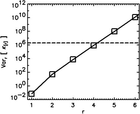
FCA allows us to determine the necessary data acquisition time by analyzing the error statistics. For example, assume that a protein with a brightness of ɛ₁ = 2 associates to form dimers with a brightness of ɛ₂ = 4. The data sampling time is T = 20 μs and the average number of molecules for each species is expected to be N₁ = N₂ = 3. How many data points are needed to resolve this mixture? We take the parameters, ɛ₁, N₁, ɛ₂, N₂, and calculate the relative variance assuming a single data point (n = 1) (Fig. 9). The variance and the relative variance are inversely proportional to the number of data points n. A minimum of four statistically significant cumulants is necessary to resolve two species. Since four cumulants are required for resolving the mixture, a line is drawn vertically in Fig. 9, so that the first four cumulants are below the line. The value of the reduced variance corresponding to that line determines the number of data points needed to acquire the desired signal statistics, because the variance is inversely proportional to the number of data points, (Eq. 41). For example, about n = 2 × 10⁶ data points are required to resolve the binary mixture. The total data acquisition time needed is given by t_DAQ = nT.

FIGURE 9.

Calculation of the relative variance Var_r of a binary mixture for a single data point (n = 1). The calculation is based on the following parameters, ɛ₁ = 2, ɛ₂ = 4, and N₁ = N₂ = 3. A dashed line is drawn horizontally, so that four cumulants lie below it. The relative variance of the line is 2 × 10⁶, which corresponds to the number of data points required to achieve four statistically significant cumulants.

Another advantage of FCA over PCH is its close relationship to correlation functions. This relationship allows the calculation of cumulants for arbitrary sampling times. We demonstrated this approach for the second integrated intensity cumulant (Eq. 22). Theory and experimental data are in very good agreement (Fig. 7). We determine the molecular photon-count rate, the diffusion time, and the aspect ratio of the beam profile by fitting the experimental data. Initially, at short data acquisition times the curve in Fig. 7 has a linear slope, which corresponds to the situation, where the integrated intensity fluctuations track the intensity fluctuations and the brightness is proportional to the data sampling time, ɛ = λT. The slope of the brightness curve decreases for larger data sampling times, because some fluorophores diffuse out of the observation volume during the sampling time, which imposes a limit on the number of collected photon counts per molecule.

PCH is only correct as long as the sampling time is short compared to the diffusion time through the observation volume. Finding an exact solution for PCH for large sampling times has been difficult. However, there has been an approach described in the literature that extends histogram analysis to longer sampling times (Palo et al., 2000). The model, called FIMDA, is based on an approximation, where correction factors for the brightness and the number of molecules are determined from the rebinned second intensity cumulant. Higher moments are not corrected for in this model. Cumulant analysis is advantageous because it offers an exact approach for taking arbitrary sampling times into account. Here, we only corrected the second cumulant to illustrate the technique.

CONCLUSIONS AND SUMMARY

This manuscript introduces FCA, a new analysis technique that extracts information from cumulants of fluorescence fluctuation data. We describe a simple model that connects the brightness and number of molecules of fluorescent species with the factorial cumulants of photon counts. In addition, we developed error analysis by introducing equations for the variance of factorial cumulants. Comparison of FCA with PCH shows that both techniques lead to identical results. Thus, FCA presents an alternative analysis technique for resolving species through brightness differences. FCA has some advantages over PCH. A straightforward mathematical model describes the factorial cumulants and allows a simple algorithmic implementation. In addition, calculation of the relative error of cumulants answers the question whether the signal statistics of the data is sufficient for resolving heterogeneous samples. The theory of cumulants also provides an approach for analyzing fluorescence fluctuation data taken with arbitrary sampling times. We derived expressions for the second factorial cumulant for arbitrary sampling times and demonstrated that theory and experiment agree. This approach can increase the sensitivity of FCA in resolving species significantly. The demonstration and analysis of higher order cumulants with arbitrary sampling times will be the subject of a separate study.

APPENDIX A

Let us consider for the moment a single, diffusing molecule with brightness ɛ in a large, but closed volume V. The r^th integrated fluorescence intensity moment for that single molecule 〈W^r〉⁽¹⁾ is, according to Eq. 4, given by

(28)

where the probability p(→) to find the molecule at location → is given by p(→) = 1/V.

The cumulants and raw moments are related by Kendall and Stuart (1977a),

(29)

where the second summation extends over all non-negative π- and ρ-values, subject to and Equation 29 states that the r^th integrated intensity cumulant of a single molecule is given by the r^th raw moment 〈W^r〉⁽¹⁾ plus a sum of products of raw moments. Because each integrated intensity moment 〈W^r〉⁽¹⁾ is proportional to 1/V, every product of intensity moments is proportional to 1/V^m, with m ≥ 2. We insert Eq. 28 into Eq. 29 and express the r^th integrated intensity cumulant as

(30)

The explicit expression of the functions f_m(ɛ) is not of interest here, but can be explicitly constructed from Eqs. 28 and 29.

If there are N_total molecules in the sample with volume V, then the r^th intensity cumulant is given by the sum of over all molecules in the sample as

(31)

The concentration of the sample is given by We rewrite Eq. 31 as

(32)

In fluorescence fluctuation experiments we measure fluorescence emerging from an open excitation volume, which is much smaller than the total sample volume V. We express the assumption of a very large surrounding volume, by taking the limit 1/V → 0. Note that the concentration of the sample, which is an intensive quantity, is unchanged. The r^th integrated intensity cumulant is now given by

(33)

In the last step, we used Eq. 8 to express the concentration c in terms of the average number of molecules N in the PSF volume V_PSF, as is customary in fluorescence fluctuation spectroscopy. This derivation follows very closely arguments presented by Qian and Elson (1990b) for deriving the first four cumulants. We extended their argument to cumulants of arbitrary order.

APPENDIX B

Fluorescence fluctuation experiments measure a sequence of photon counts (k₁,k₂,…k_n). Any statistics of the experiment is based on this random sample of size n. The moments and cumulants of the experimental photon counts are called sample moments and sample cumulants. Repeated measurements of a sample produce different sequences of photon counts and therefore slightly different sample moments. The distribution of the sample moments is described by the statistics of sampling distributions, which connects experiment and theory.

The k-statistics of a sample distribution provides an unbiased estimator of population cumulants (Fisher, 1928). The r^th k-statistic k_r is the unique, symmetric, and unbiased estimator of the r^th population cumulant κ_r, E[k_r] = κ_r. Factorial cumulants are given by a linear combination of cumulants,

(34)

The coefficients C_i may be looked up or calculated from the relationship between their generating functions (Kendall and Stuart, 1977b). We construct an unbiased estimator k_[r] of factorial cumulants κ_[r] by replacing the population cumulants κ_r with their corresponding k-statistics,

(35)

The expectation value of k_[r] is equal to the factorial cumulant,

To construct explicit expressions of the unbiased estimator k_[r], Eq. 35 is evaluated after expressing k-statistics in terms of power sums s_r (Kendall and Stuart, 1977b),

(36)

For example, the unbiased estimator k_[2] of the second factorial cumulant is

(37)

We need to calculate the variance of the factorial cumulant estimator k_[r],

(38)

Explicit expressions of the variance are obtained from Eq. 38 by converting k_[r] into augmented symmetrics, followed by the application of the fundamental expectation result (Kendall and Stuart, 1977b; Rose and Smith, 2002b). We use the software program MathStatica for determining expressions of the variance. For example, the variance of k_[2] expressed in terms of population cumulants is

(39)

The number of data points n of our experimental data sets tends to be very large (n is on the order of 10⁶). This allows us to simplify the equations by formally taking the limit of n → ∞,

(40)

The variance function expresses the hypothetical variance for a single data point. The variance for a sample of n data points, where n is large, is then approximated by

(41)

We calculated the variance of factorial cumulants by the method described. Explicit expressions of the variance of the first three factorial cumulants are given in Eq. 14. We also report here the variance of the fourth and fifth factorial cumulants:

(42)

The variance of factorial cumulants of higher order are calculated as well, but the resulting equations are too lengthy to be reported here.

References

- Bevington, P. R., and D. K. Robinson. 1992. Data Reduction and Error Analysis for the Physical Sciences. McGraw-Hill, Boston, MA.
- Chen, Y., J. D. Müller, P. T. C. So, and E. Gratton. 1999. The photon counting histogram in fluorescence fluctuation spectroscopy. Biophys. J. 77:553–567. [DOI] [PMC free article] [PubMed] [Google Scholar]
- Chen, Y., L. N. Wei, and J. D. Müller. 2003. Probing protein oligomerization in living cells with fluorescence fluctuation spectroscopy. Proc. Natl. Acad. Sci. USA. 100:15492–15497. [DOI] [PMC free article] [PubMed] [Google Scholar]
- Fisher, R. A. 1928. Moments and product moments of sampling distributions. Proc. Lond. Math. Soc. 30:199–238. [Google Scholar]
- Hess, S. T., S. Huang, A. A. Heikal, and W. W. Webb. 2002. Biological and chemical applications of fluorescence correlation spectroscopy: a review. Biochemistry. 41:697–705. [DOI] [PubMed] [Google Scholar]
- Hillesheim, L. N., and J. D. Müller. 2003. The photon counting histogram in fluorescence fluctuation spectroscopy with non-ideal photodetectors. Biophys. J. 85:1948–1958. [DOI] [PMC free article] [PubMed] [Google Scholar]
- Kask, P., K. Palo, D. Ullmann, and K. Gall. 1999. Fluorescence-intensity distribution analysis and its application in biomolecular detection technology. Proc. Natl. Acad. Sci. USA. 96:13756–13761. [DOI] [PMC free article] [PubMed] [Google Scholar]
- Kendall, M. G., and A. Stuart. 1977a. Moments and cumulants. In The Advanced Theory of Statistics, Vol. 1. MacMillan Publishing, New York. 57–96.
- Kendall, M. G., and A. Stuart. 1977b. Cumulants of sampling distributions. In The Advanced Theory of Statistics, Vol. 1. MacMillan Publishing, New York. 293–328.
- Mandel, L. 1958. Fluctuations of photon beams and their correlations. Proc. Phys. Soc. 72:1037–1048. [Google Scholar]
- Medina, M. A., and P. Schwille. 2002. Fluorescence correlation spectroscopy for the detection and study of single molecules in biology. Bioessays. 24:758–764. [DOI] [PubMed] [Google Scholar]
- Meseth, U., T. Wohland, R. Rigler, and H. Vogel. 1999. Resolution of fluorescence correlation measurements. Biophys. J. 76:1619–1631. [DOI] [PMC free article] [PubMed] [Google Scholar]
- Müller, J. D. 2003. Following protein association in vivo with fluorescence fluctuation spectroscopy. SPIE Biomed. Optics. 4963:24–31. [Google Scholar]
- Müller, J. D., Y. Chen, and E. Gratton. 2000. Resolving heterogeneity on the single molecular level with the photon counting histogram. Biophys. J. 78:474–486. [DOI] [PMC free article] [PubMed] [Google Scholar]
- Müller, J. D., Y. Chen, and E. Gratton. 2003. Fluorescence correlation spectroscopy. In Methods of Enzymology. G. Marriott and I. Parker, editors. Academic Press, San Diego, CA. 69–92. [DOI] [PubMed]
- Palmer, A. G. D., and N. L. Thompson. 1987. Molecular aggregation characterized by high order autocorrelation in fluorescence correlation spectroscopy. Biophys. J. 52:257–270. [DOI] [PMC free article] [PubMed] [Google Scholar]
- Palmer, A. G. D., and N. L. Thompson. 1989. High-order fluorescence fluctuation analysis of model protein clusters. Proc. Natl. Acad. Sci. USA. 86:6148–6152. [DOI] [PMC free article] [PubMed] [Google Scholar]
- Palo, K., U. Mets, S. Jager, P. Kask, and K. Gall. 2000. Fluorescence intensity multiple distributions analysis: concurrent determination of diffusion times and molecular brightness. Biophys. J. 79:2858–2866. [DOI] [PMC free article] [PubMed] [Google Scholar]
- Qian, H., and E. L. Elson. 1990a. Distribution of molecular aggregation by analysis of fluctuation moments. Proc. Natl. Acad. Sci. USA. 87:5479–5483. [DOI] [PMC free article] [PubMed] [Google Scholar]
- Qian, H., and E. L. Elson. 1990b. On the analysis of high order moments of fluorescence fluctuations. Biophys. J. 57:375–380. [DOI] [PMC free article] [PubMed] [Google Scholar]
- Rose, C., and M. D. Smith. 2002a. Continuous random variables. In Mathematical Statistics with Mathematica. Springer, New York. 31–80.
- Rose, C., and M. D. Smith. 2002b. Moments of sampling distributions. In Mathematical Statistics with Mathematica. Springer, New York. 251–276.
- Saleh, B. 1978. Point processes. In Photoelectron Statistics With Applications to Spectroscopy and Optical Communication. Springer-Verlag, Berlin, Germany. 57–84.
- Schätzel, K. 1987. Correlation techniques in dynamic light scattering. Appl. Phys. B. 42:193–213. [Google Scholar]
- Thompson, N. L. 1991. Fluorescence correlation spectroscopy. In Topics in Fluorescence Spectroscopy. J. R. Lakowicz, editor. Plenum Press, New York. 337–378.
- Thompson, N. L., A. M. Lieto, and N. W. Allen. 2002. Recent advances in fluorescence correlation spectroscopy. Curr. Opin. Struct. Biol. 12:634–641. [DOI] [PubMed] [Google Scholar]
- Van Craenenbroeck, E., and Y. Engelborghs. 2000. Fluorescence correlation spectroscopy: molecular recognition at the single molecule level. J. Mol. Recogn. 13:93–100. [DOI] [PubMed] [Google Scholar]
- van Kampen, N. G. 1981. Stochastic Processes in Physics and Chemistry. North-Holland, Amsterdam, The Netherlands.